Recognition of Physical Activities from a Single Arm-Worn Accelerometer: A Multiway Approach

Abstract

In current clinical practice, functional limitations due to chronic musculoskeletal diseases are still being assessed subjectively, e.g., using questionnaires and function scores. Performance-based methods, on the other hand, offer objective insights. Hence, they recently attracted more interest as an additional source of information. This work offers a step towards the shift to performance-based methods by recognizing standardized activities from continuous readings using a single accelerometer mounted on a patient’s arm. The proposed procedure consists of two steps. Firstly, activities are segmented, including rejection of non-informative segments. Secondly, the segments are associated to predefined activities using a multiway pattern matching approach based on higher order discriminant analysis (HODA). The two steps are combined into a multi-layered framework. Experiments on data recorded from 39 patients with spondyloarthritis show results with a classification accuracy of 94.34% when perfect segmentation is assumed. Automatic segmentation has 89.32% overlap with this ideal scenario. However, combining both drops performance to 62.34% due to several badly-recognized subjects. Still, these results are shown to significantly outperform a more traditional pattern matching approach. Overall, the work indicates promising viability of the technique to automate recognition and, through future work, assessment, of functional capacity.

1. Introduction

Monitoring of chronic diseases has received a lot of attention over the last decade. One such disease is (axial) spondyloarthritis (axSpA). Its symptoms include inflammation of the spinal region, sometimes also the extremities. Eventually, ossification of the spine may occur, severely limiting a patient’s functional capacity and general mobility. The disease is treated with anti-inflammatory drugs, but physical therapy and exercising are an equally important part of the treatment [1]. Moreover, physical therapy and exercises yield insight into the remaining functional capacity. This information complements disease activity, judged from, among others, MRI scans or protein levels in blood samples [2]. Standard exercises include e.g., stretching, core stability exercise, muscle strengthening and exercises mimicking activities of daily living (ADL). These are judged subjectively by the physician or therapist. In addition, functional capacity is rated by the patient himself using patient questionnaires such as the Bath Ankylosing Spondylitis Functional Index (BASFI) [3]. More recently, the interest in objective performance-based methods has risen. The simplest way to achieve an objective quantification is timing e.g., using a chronometer. However, this can easily be automated via patient monitoring and has proven to be significant [4,5]. A key step in computing duration or other performance-related features automatically is the detection and recognition of the relevant activities from a continuous datastream. This has the additional advantage that the monitoring can be moved to a home environment and the physician can be provided with the data to track a patient’s evolution.

In the past, physical activity recognition often suffered from several disadvantages due to the available technology and the required computational power. For example, vision-based approaches have been available for some decades and continue to be used, but they are subject to spatial restrictions. Moreover, they are sensitive to specific problems such as lighting conditions. Nevertheless, they have obtained good results in e.g., visual surveillance and human computer interaction [6,7].

Since then, new options became available with the advent of relatively cheap wearable technology. These sensors are attached to the user’s body and can be applied in everyday situations rather than in limited setups. This is of particular importance in patient or elderly monitoring. Data acquisition can more easily be moved into the home environment.

Different kinds of sensors have been used, many of them multimodal. Accelerometers, measuring linear accelerations, are very common. They are also often combined with gyroscopes, supplying angular velocities, and magnetometers, yielding changes in magnetic fields, in an inertial (magnetic) measurement unit (IMU). Additionally, GPS can be incorporated as well. Although adding sensors yields more, potentially valuable, information, this has to be weighted against power consumption, a major concern in wearables, particularly when measuring over longer periods of time. High-energy batteries still tend to be bulky and cumbersome [8], whereas miniaturization is a key concept in wearable technology. Within these limits, many applications have been designed. As an example, full-body motion capture can be achieved using many sensors to track the movement of all body parts [9]. Furthermore, several studies have used accelerometers to study energy expenditure and sedentary behaviour over longer periods of time [10,11,12,13,14,15].

The latter is a common example of long-term monitoring. This approach can be extended to include recognition of ADL such as sitting, walking, running, cycling etc. [16,17,18,19,20]. This is of potential interest to construct personal profiles and to improve general health. Sliding windows are a common technique for this kind of recognition. First, a window length and a step size for window advancement over the measured signals are (e.g., multi-channel accelerometry) are defined. Then, from each window, features can be extracted. A classifier can be trained based on these features to attribute an activity label to every window. Many studies follow this approach, but there is a lot of variability in its implementation. Studies vary in, for example, which and how many sensors are being used, the positioning of the sensors on the body, the window length and overlap, the time/frequency/wavelet features extracted from each window and the choice of classifier [21,22]. No consensus seems to exist as to what is the best possible setup, although comparisons in specific cases offer some conclusions [23,24]. It can be assumed this depends on the activities under consideration. Yet, good results have been obtained with several setups. The studies agree that the number of sensors should be limited for users’ convenience [25,26,27].

Despite the progress in activity recognition, the techniques mentioned above are ill-suited to detect the activities under consideration for assessment of functional capacity. They are short and transitional in contrast to the repetitive longer nature of e.g., walking, running or cycling. Therefore, a pattern-matching approach is more effective than the common sliding windows [28]. Some window-based studies do include transitions, but in a strongly restricted setup e.g., with 40 s quiet sitting or standing to separate activities [29]. Pattern approaches have been used before in limited setting, for example to recognize the occurrence of sit-to-stand transitions [30]. The limited setting stems from the fact that the problem is particularly difficult. In any realistic setting many non-informative movements occur and should be rejected. Hence, patterns should capture enough variance inherently present in the activity, but still be discriminative towards non-informative activities. When dealing with patients, this variability is even more pronounced as compared to healthy subjects [31,32]. Mostly, the necessary variability in patterns is captured via Dynamic Time Warping (DTW), allowing the signal to adapt to a pattern [33,34]. Another possibility is decomposing activities in simple motion primitives and applying a bag-of-features model [35].

In order to recognize patterns in the data, they should first be detected. This is challenging because many similar shapes due to activities that are not of interest are most likely part of the data. Moreover, activities are not always well separated from each other e.g., a subject might stand up and start walking immediately. One solution, particularly suitable to sliding window approaches, is merging the stages of detection and recognition. This technique adds a specific rejection class to the data and processes it as any other class [28]. Alternatively, detection can be dealt with implicitly using Hidden Markov Models (HMM) [36]. It can also be modelled explicitly based on signal energy [37] or using a multi-resolution segmentation based on prior knowledge of the expected length of all activities [38].

The effectiveness of both detection and recognition can be improved by taken into account structure and interdependence of the data. For example, accelerometers measure along several axes. Moreover, similarities between activities can also be used to improve their contrast to other activities. Once the data is converted to a multiway structure (tensor), more elaborate feature extraction methods such as Higher Order Discriminant Analysis (HODA) can be used. This technique was introduced in the last decade and has proven very successful in fields as diverse as image classification, brain-computer interfaces and handwritten digit recognition [39].

This paper describes a novel approach for automatic detection and recognition of activities related to functional capacity in axSpA patients from a single arm-worn accelerometer. It aims to show the structure of the data can be exploited and has added value on top of the common DTW matching when combined with HODA. To this end the stages of detection (segmentation) and recognition are addressed and assessed, both independently and jointly. The obtained results are intended as a step towards assessment of functional capacity in the home environment.

2. Materials and Methods

This Section starts with a description of the data collected in the University Hospital of Leuven. Next, it discusses the tensorial data representation based on dynamic time warping (DTW). It allows to use higher order discriminant analysis (HODA) as feature selection approach. Simple pattern matching features will be introduced as well as a benchmark. Once all these building blocks are in place, the general approach for both detection and recognition can be outlined. Finally, the Section ends by describing the performed experiments.

2.1. Data

Data was recorded in two sessions at different points in time. Despite the slight differences between the two sessions discussed below they were pooled to increase the sample size and to study the impact of heterogeneous conditions. The merged dataset includes patients diagnosed with axial spondyloarthritis (axSpA) as defined by the ASAS classification criteria [40], verified by an expert rheumatologist at the University Hospitals, Leuven. The acquisition protocol was approved by the Medical Ethics Committee of the University Hospitals Leuven (ML 5236). All test subjects provided written informed consent before participating. Both recordings took place at the Division of Rheumatology, University Hospitals, Leuven.

In total, 39 patients were measured, 23 male and 16 female. The patients’ average functional capacity, estimated using the BASFI score, was 3.16/10, with higher values indicating a decreased capacity. All patients were equipped with a 32Hz accelerometer mounted on the biceps of the right (dominant) arm to record acceleration across the longitudinal and the transversal axes. This position was chosen as a compromise between arm and body movement. On the one hand, it is on the upper arm which implies it can capture activities such as reaching. On the other hand, it remains close to the center of mass of the patient and captures mostly the general movement of the body. In contrast, positioning on e.g., the wrist would allow more details on arm movements, but its higher degrees of freedom due to the longer kinematic chain obscure whole-body movements.

The protocol consisted of the patients performing a series of physical tasks based on the BASFI questionnaire in a randomized order. Each task was performed twice to provide test-retest reliability. After an initial validity study on the first data set [5], six tests remained.

Table 1. Abbreviation and descriptions of the six activities performed in the experimental protocol. The last column shows how many patients performed the activity.

Activity	Description	# Patients
getUp	getting up starting from lying down	39
lieDown	lying down from stance	28
maxReach	reaching up as high as possible	28
pen5	picking up a pen five times as quickly as possible	39
reach5	reaching up five times as quickly as possible	39
sts5	sit-to-stand from a chair 5 times as quickly as possible	39

presents a summary of the activities. As can be seen, half of the selected activities are repeated five times. In combination with the maximum speed requirement, this minimizes the test-retest variability.

Labels for training and testing purposes were obtained by manual segmentation and labelling performed by students of the Faculty of Rehabilitation Sciences under the supervision of a physical therapist. Directions were given beforehand and the results were checked by the therapist to minimize the impact of individual raters.

Despite the pooling of the recording sessions, two differences need to be mentioned.

• The first session, consisting of 28 patients, is recorded with a bi-axial accelerometer (Sensewear Pro 3 Armband, Bodymedia Inc., Pittsburgh, PA, USA). The remaining 11 subjects were equipped with the tri-axial Shimmer3 (Shimmer, Dublin, Ireland) since the Sensewear sensor had been discontinued. Two Shimmer axes were selected to correspond to the Sensewear setup. The remaining axis was left out.
• In the second recording, only four out of six selected activities were performed, lieDown and maxReach were not present. Nevertheless, all six activities are included in the study to allow for a wider variability. Table 1 indicates the number of patients that performed the activity in its last column.

2.2. Data Representation

The data representation consists of two steps: defining relevant activity patterns from training data and transforming data based on these patterns to a tensorial representation. Figure 1 summarizes the approach. Alternatively, simple features can be derived directly after the pattern matching step, as discussed at the end of this Section. Throughout, data are assumed to be available as annotated segments, rather than as a continuous acceleration datastream. How to derive these segments will be discussed in Section 2.4.

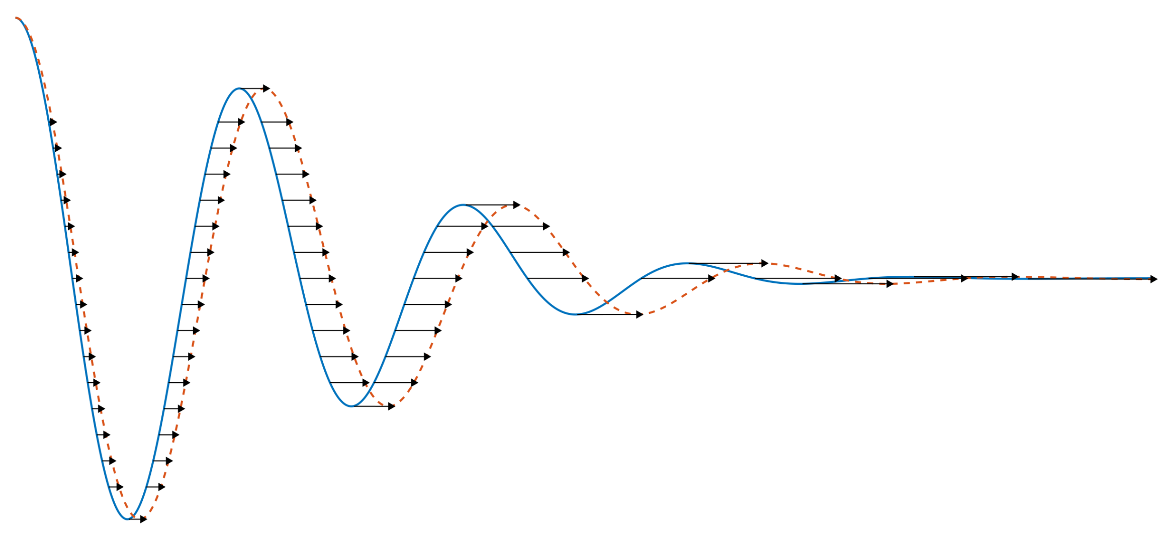
2.2.1. Pattern Definition with Dynamic Time Warping (DTW)

A general pattern for every activity can be constructed from training data segments by means of dynamic time warping (DTW). The basic implementation has been applied for decades. It matches two signals, possibly of different lengths, by stretching them to minimize a cost function e.g., the Euclidean distance between the warped curves [41]. Figure 2 shows an example for two damped sinusoidals with slightly different frequencies. As can be seen, DTW scales shapes along the length of the signal, but because of this it can be prone to errors when large amplitude differences occur. Extension techniques such as derivative dynamic time warping have been introduced to alleviate this issue [42]. In the current setup however, the shape differences stem from the change in orientation, that is, the gravity component of the acceleration. It has the same amplitude for all subjects performing an activity, except when slight pose differences occur. Therefore, DTW extensions have not been considered.

In order to use DTW to construct a pattern for each activity in the current setup, two DTW extensions are needed. Firstly, each trial consists of two channels instead of one. They have to be matched jointly between channels (multi-channel matching). Secondly, more than two segments should be matched to obtain common patterns over all training data (multi-segment matching). This has been implemented in a Matlab toolbox by Zhou and De la Torre [43]. Therefore, if training data has been selected, six patterns can be derived by applying DTW once for all segments belonging to the same activity class. Each pattern consists of two pattern channels.

2.2.2. Simple Pattern Features

Tensorizing the matched data increases the complexity of the algorithm, as discussed further. Simpler pattern matching features are proposed as an alternative for comparison to assess the added value of the tensors. They are extracted at the layer of the deformed segments in Figure 1. At that layer, training or test segments are matched against the patterns. For each match, DTW provides an euclidean distance measure to assess the similarity between the warped segment and the template. Overall, this yields a distance for every activity class pattern per segment. Hence, these distances can be used directly as feature vector. Starting from the derived activity patterns, the approach can be summarized as follows, both for training and unknown, new, segments:

• Match the segment to an activity pattern using DTW. This is a simple match between the two-channel segment and a two-channel pattern. Its result is a two-channel deformed segment and a distance score.
• Repeat the first step for all activity patterns.

It is possible to directly derive the class label from the feature vector by a simple approach: the minimal distance to a pattern most probably points to the associated class as label. Yet, all distances together yield more information than only this minimum. Therefore, the full feature vector will be used as benchmark for further analysis.

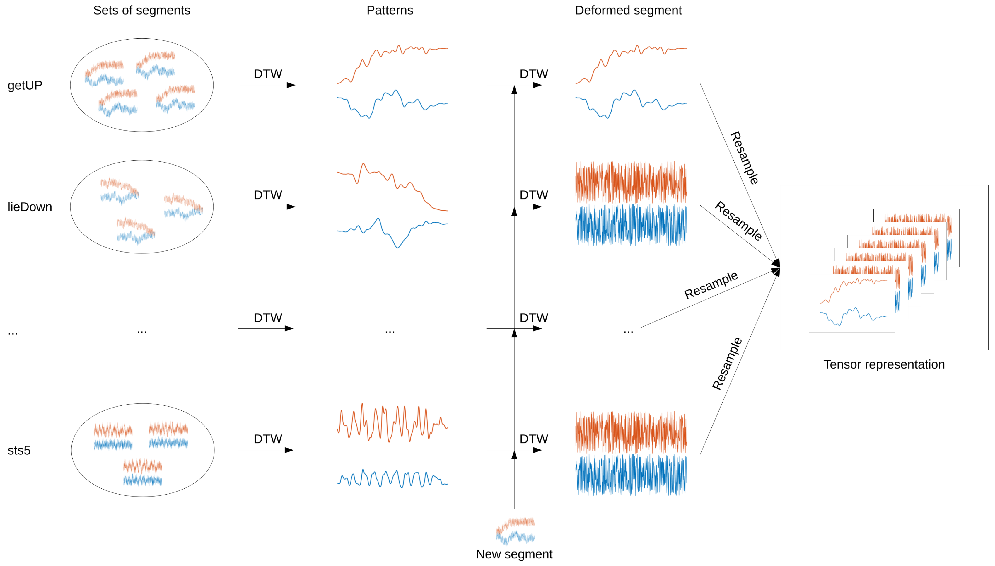
2.2.3. Tensor Construction from Activity Patterns

Tensors are a data construct in multilinear algebra, an extension of matrices [44]. A tensor has multiple modes. For example, a single-mode (or one-way) tensor with n elements is a vector denoted with a bold character $\mathbf{z}\in {\mathbb{R}}^n$. A dual-mode (two-way) tensor is a matrix, e.g., with n rows and m columns, denoted with a bold capital $\mathbf{A}\in {\mathbb{R}}^{n\times m}$. Stacking l such matrices yields a tensor $\mathcal{A}\in {\mathbb{R}}^{n\times m\times l}$, called a three-way tensor or, alternatively, a tensor of order three. Such a general tensor is represented by a calligraphic font.

Starting from the activity patterns defined earlier, a tensorial representation for any activity segment is constructed in four steps.

• Match the segment to an activity pattern using DTW. This is a simple match between the two-channel segment and a two-channel pattern. Its result is a two-channel deformed segment.
• Repeat the first step for all activity patterns.
• Resample all deformed segments to a common length. A length of 150 samples was empirically selected for this study.
• Stack all resampled deformed segments into a time × channel × activity tensor. Here, this yields a $150\times 2\times 6$ tensor.

The reasoning behind the approach is as follows. If segments represent a certain activity, the match between DTW and the pattern will be good and the deformed signal will still resemble the pattern. On the other hand, deformations to match other activity patterns will be more random. Hence, the constructed tensor contains information about how well a segment resembles each of the activities. This is captured in the simple DTW features mentioned before, but they compress information into a single variable per activity, whereas the tensor approach preserves more localized similarity information.

2.3. HODA Features

A tensor is classified into an activity class based on features extracted from it using Higher Order Discriminant Analysis (HODA) features. HODA combines multilinear subspace methods with Fisher’s discriminant analysis to solve a special case of the Tucker decomposition [39]. The implementation is provided in the Novel tensor toolbox for Feature Extraction and Applications (NFEA) [45] which requires the use of the tensor toolbox by Kolda and Bader [46].

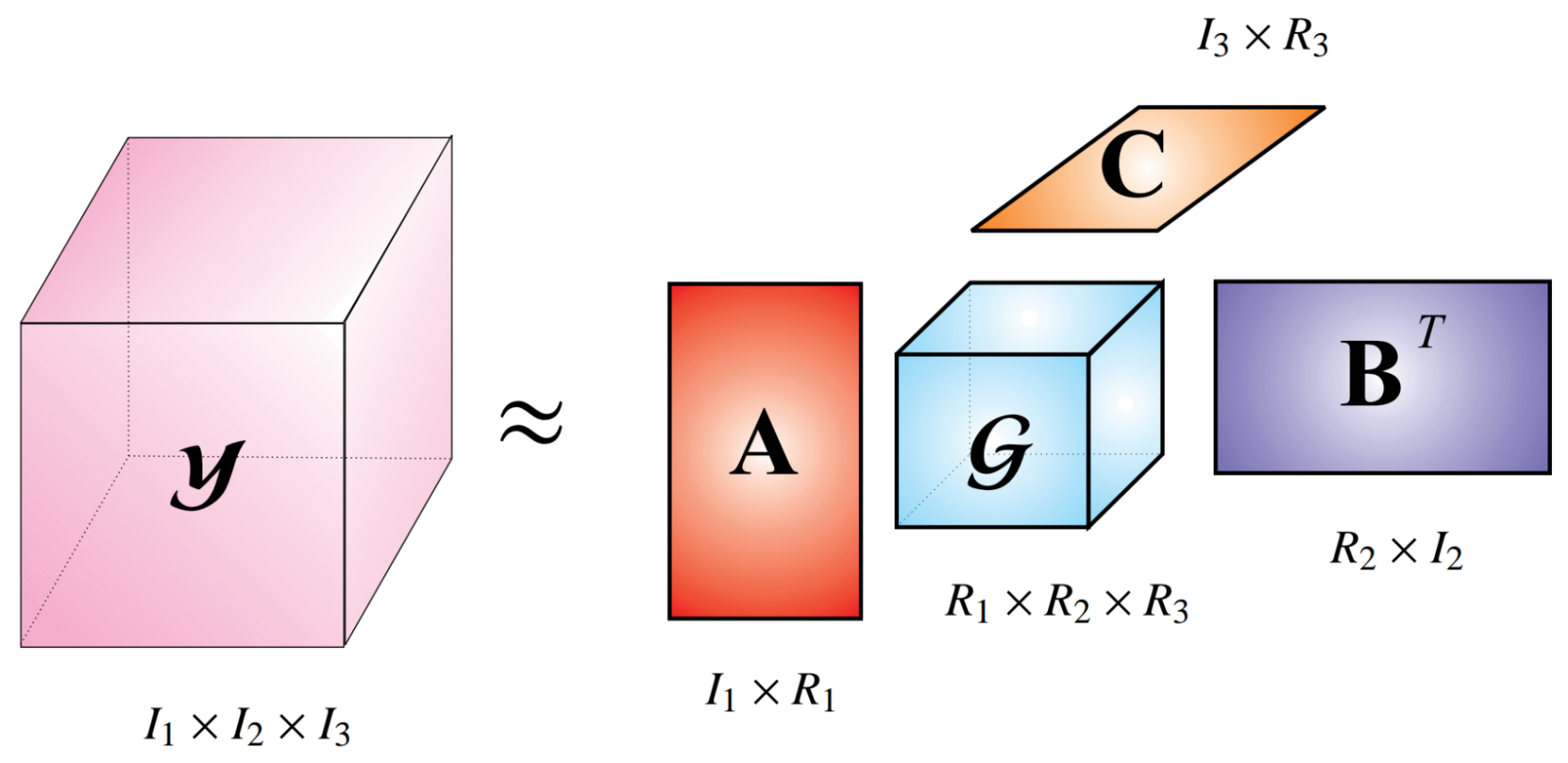
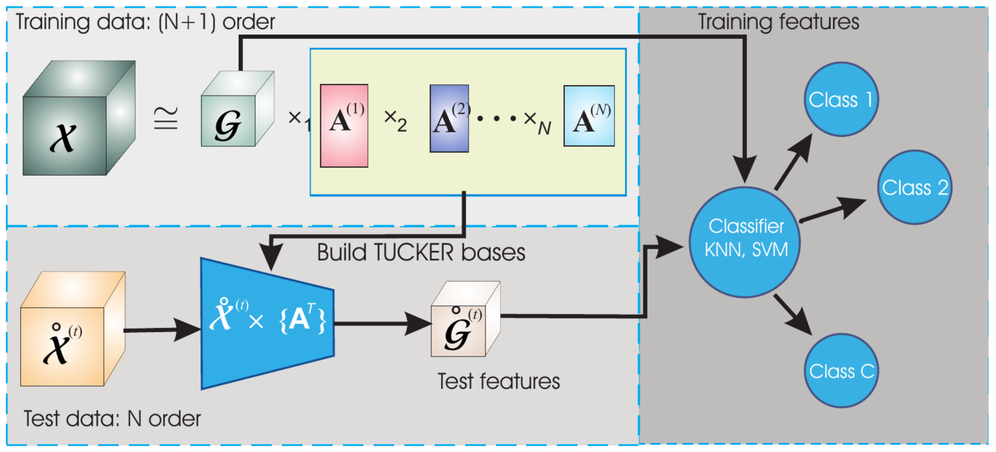
2.3.1. Tucker Decomposition

The Tucker decomposition decomposes a tensor $\mathcal{Y}\in {\mathbb{R}}^{I_1\times I_2\times I_3}$ into a smaller tensor, called the core tensor, and factor matrices. The principle is illustrated in Figure 3. The core tensor $\mathcal{G}\in {\mathbb{R}}^{R_1\times R_2\times R_3}$ is multiplied by matrices $\mathbf{A}\in {\mathbb{R}}^{I_1\times R_1}$, $\mathbf{B}\in {\mathbb{R}}^{I_2\times R_2}$ and $\mathbf{C}\in {\mathbb{R}}^{I_3\times R_3}$ along the first, second and third mode, respectively. Mode-1 and mode-2 multiplication are equivalent to left and right multiplication in case of matrices. In general, mode-n multiplication will be indicated by ${\times }_n$. Hence, the Tucker decomposition in Figure 3 can be written as:

$$\mathcal{Y}=\mathcal{G}{\times }_1\mathbf{A}{\times }_2\mathbf{B}{\times }_3\mathbf{C}+\mathcal{E}$$

(1)

In which $\mathcal{E}\in {\mathbb{R}}^{I_1\times I_2\times I_3}$ is an error term.

Equation (1) is a decomposition because it expresses the content of a tensor as a combination of interactions of vectors, namely, the columns of the factor matrices. Therefore, if common factor matrices can be found for a given set of tensors, their core tensors all express the full content of the original tensors in the multilinear space spanned by the factor matrices. The elements of the core tensors are then used as discriminative features. Discovering such common factor matrices in a class-informed way is the goal of the algorithm called HODA, discussed next.

2.3.2. Higher Order Discriminant Analysis (HODA)

HODA aims to construct common factor matrices by jointly decomposing a set of N-way tensors. This can be achieved with an explicit joint formulation, but the more common and elegant way is the formulation in terms of a decomposition of a single tensor of order $N+1$. That is, it has been shown that stacking all tensors along an additional mode and performing a Tucker decomposition disregarding the factor matrix of this last mode is equivalent to the joint formulation [39]. Such a decomposition is in general not unique. However, uniqueness can be enforced by constraints such as orthogonality or nonnegativity. HODA finds common orthogonal factor matrices via an iterative procedure attempting to maximize Fisher’s ratio [39] based on the class labels. A full mathematical derivation is outside the scope of this paper.

Once the common factor matrices have been found, the individual core tensors resulting from the original tensor observations can be vectorized and serve as training features. Moreover, the factor matrices can be used on new observations, e.g., test data, to find the core tensor and hence test features. These features can subsequently be used with any classification approach. The full HODA procedure is presented graphically in Figure 4. The graphical depiction is limited in its possibility to express N-way tensors for $N>3$. Therefore, all higher-order tensors are represented as cubes.

2.4. Detection and Recognition

So far, the focus has been on the building blocks for activity recognition starting from accelerometer segments. Yet, this first requires detecting these segments in continuous data streams. The process consists of two steps. Firstly, potential segments of interest are detected. This process is independent of any features (simple or HODA) used for further stages. Secondly, non-informative segments should be discarded.

2.4.1. Segment Identification

Segments of interest are identified by looking at the signal variability. The dynamic regions of the signal are subsequently separated from the more static ones. This separation was implemented as a step-wise adaptive approach [47].

• The continuous data is filtered with a low-pass butterworth filter of the fourth order, with a cut-off frequency of 1.6 Hz. This corresponds to 10% of the signal bandwidth. To judge the general movement pattern, low frequencies are the most important ones.
• A rough segmentation splits the signal into windows of two seconds, with 50% overlap. Segments are marked as dynamic based on their standard deviation and range, compared to empirical thresholds obtained from preliminary analysis of the training data.
• Refinement of the dynamic regions is achieved by shrinking or extending the static regions in between dynamic segments based with half a second. The decision is based on the difference in variance between half-second regions and is identical for the start and end of a region, so the discussion will be limited to the start. The initial second of a static region serves as baseline. Extension is accepted if the second starting at half a second before the current start has a variance which is maximally 10% higher than the baseline. This tries to grow the static region without incorporating too much movement. Shrinking is accepted if the variance of the second starting at half a second later than the current start is at least 10% lower. This tries to eliminate movement at the start of the region.
• The above procedure is carried out independently for different channels. The detected dynamic regions are subsequently joined over all channels. Static gaps of less than a second in between dynamic regions are discarded if the means of the regions are similar. As a last step, dynamic regions of less than two seconds are discarded.

2.4.2. Rejection

Rejection involves discarding segments representing activities that are of no interest in this study. It is challenging because the rejection class is heterogeneous and cannot always be fully known beforehand since patients can perform any movement, whereas for the activity classes, their general characteristics are known. A workaround is the use of a one-class classifier for each class of interest. In this case however, an estimate of the data to be discarded is available from training data.

For every patient, the informative segments are known in the continuous dual-channel acceleration signals. Hence, if the segmentation is run, all segments not overlapping with the known activities are examples of the rejection class. In other words, this allows to increase the set of known segments and labels for each patient by introducing a rejection class label. Therefore, the problem can simply be solved as a classical multi-class approach. A random forest with 250 trees was selected for its ability to model complex boundaries [48]. A uniform prior was imposed to avoid too strong a bias towards the rejection class. Individual trees were constructed by random resampling of the data with an in-bag-fraction of $0.65$. Other than that, standard settings in Matlab’s TreeBagger have been used.

2.5. Experiments

All experiments were performed in Matlab R2017b (The Mathworks, Natick, MA, USA). Three aspects of the approach were tested. A first experiment solely focuses on recognition, that is, it starts from already segmented data with given class labels. A second experiment assesses the segmentation approach, neglecting any class labels. Finally, the third experiment brings together segmentation and classification. The first and the third experiment include a comparison between the methods applied on simple features or HODA features. The statistical significance of the results of this comparison is assessed with a sign test, a non-parametric test for the difference of medians of two populations, implemented by Matlab’s signtest.

2.5.1. Recognition

To evaluate recognition only, a ‘closed world’ scenario is used. All activities are available as segments and all available segments can only be one of the six classes listed in Table 1. Data is processed as leave-one-subject-out (LoSo). It is a crossvalidation approach consisting of 39 folds, one for each patient. In every fold, data from 38 patients is used as training data with the remaining patient as test data. The manual class identifications are used as ground truth labels.

Simple and HODA features are calculated as described in Section 2.2 and Section 2.3. Summarizing, in every fold, the following steps are carried out:

• Class-specific patterns are derived from the training data using DTW.
• Data segments, both training and test, are warped to all training class patterns. This yields deformed segments with the associated distances as simple features.
• The deformed segments are converted to a tensorial representation.
• HODA derives the discriminative subspaces and core tensors based on the training data. As toolbox parameters, the quality of the approximation is set to 98.5 and the subspaces are derived via generalized eigenvalue decomposition.
• The subspaces defined by the factor matrices are used to extract the core tensors for the test data.
• Training and test HODA features are obtained by vectorization of the core tensors.
• Test data is evaluated via a multiclass-trained linear discriminant analysis classifier (LDA) for both types of features [49].

The segments are expected to be relatively dissimilar, so a more complex classifier such as the random forest mentioned earlier is not necessary here. In contrast, it might lead to overfitting. LDA is a simple linear classifier with less hyperparameters. Due to its linear nature, it leads to more robust models. It is implemented in Matlab as fitcdiscr. Results will be assessed using accuracy per subject as well as a confusion matrix over all subjects.

2.5.2. Segmentation

Segmentation is performed for every patient as outlined in Section 2.4.1. It is expected that many segments will be found, among which also the informative ones given as training data. This experiment matches the detected segments with the given ground-truth, discarding all other detected segments. Aspects to be assessed include whether all informative segments have indeed been detected and how accurate this detection is. The latter is quantified by the Sørensen-Dice coefficient [50] (SDC). Given segments X and Y, it can be defined as:

$$\mathrm{SDC}(X,Y)=\frac{2|X\cap Y|}{\left|X\right|+\left|Y\right|}$$

(2)

It can be considered as a percentwise measure of overlap between X and Y.

Note that segmentation is independent of the type of features used later for recognition. Therefore, no comparison is provided.

2.5.3. Combination

The last experiment is similar to the first as it also runs with the LoSo setup and compares simple features to HODA features. However, as described earlier, a rejection class is introduced. Moreover, the test data segments are no longer predefined through manual delineation, but are obtained through segmentation, as in the previous experiment. The aim is to reject non-informative segments and correctly classify the others. Several measures will be used to assess the performance:

• The number of false detections FD is the amount of segments classified as belonging to one of the six classes, whereas they should be in the rejection class.
• Detection True Positive Rate (DTPR) is the ratio of the number of segments that have (correctly) been accepted and the number of actual informative segments. It is an alternative for the number of false negatives, that is, missed detections (FN). Whether segments are classified correctly is irrelevant for the DTPR, only the difference between accepted and rejection is assessed.
• The pure accuracy ACC${}_p$ is the classification accuracy when only looking at the accepted segments. This neglects the impact of FD and FN.
• The actual accuracy ACC${}_a$ is the most complete measure of performance. It is the classification accuracy taking into account both FDs and FNs as misclassifications.

3. Results

This section subsequently discusses the results of the three experiments: Recognition, Segmentation and Combination.

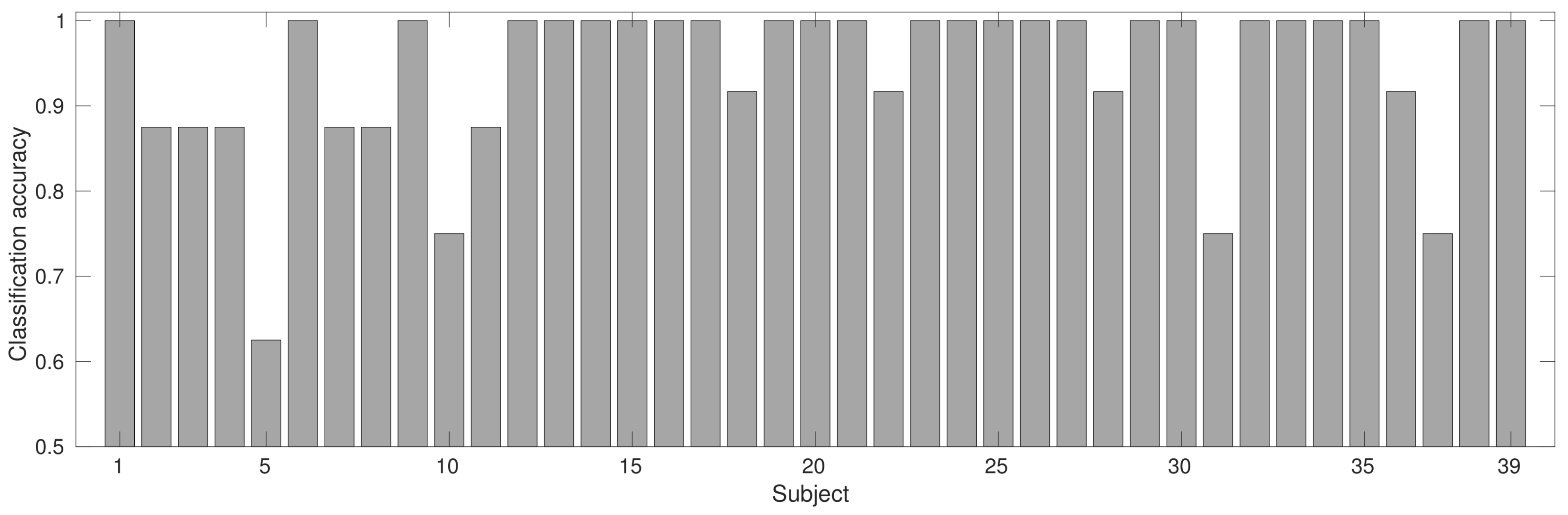
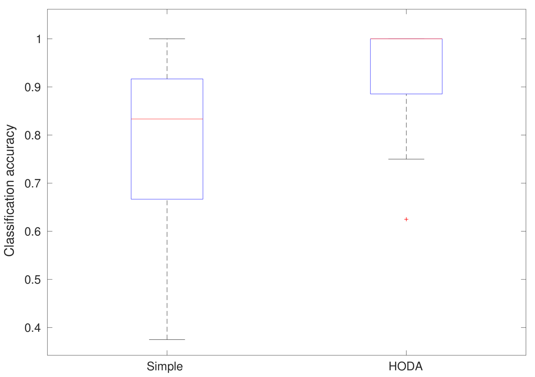
3.1. Recognition Results

Figure 5 shows a bar plot of the classification accuracy for all subjects using HODA features. The average accuracy is 94.34% (std 9.24%). Moreover, the figure shows that perfect recognition was achieved for 25 subjects. A further four subjects had accuracies higher than 90%, six others between 80% and 90% and three more between 70% and 80%. Only a single subject had an accuracy lower than 70%.

The boxplot in Figure 6 offers a comparison between the simple features and HODA. The latter outperforms the former with a highly significant difference ($p<0.01$). Simple features lead to an average classification accuracy of 78.21% (std 17.74), a difference of 16%. Only 8 subjects achieve perfect recognition.

Assessment can also be done on the level of confusion between activities. The conclusions will be illustrated for HODA, but are similar for the simple features.

Table 2. Confusion matrix of the classified activities using HODA features over all 39 subjects. Correct detections are highlighted by the gray-shaded diagonal.

		Predicted Labels
		getUp	lieDown	maxReach	pen5	reach5	sts5
Actual labels	getUp	76	0	0	0	1	1
	lieDown	0	56	0	0	0	0
	maxReach	0	0	56	0	0	0
	pen5	0	0	0	68	5	5
	reach5	0	0	0	1	76	1
	sts5	2	0	0	3	2	71

displays the confusion matrix for all activities. It shows that all occurrences of lieDown and maxReach are perfectly recognized. Moreover, they have no confusion with other activities at all. Reach5 and getUp are only missed twice. Another observation is some confusion between the repeated activities. Most importantly, pen5 is sometimes estimated to be sts5 (five occurrences) or reach5 (five occurrences). This can be explained by the fact that the movement of the arm is similar in these cases.

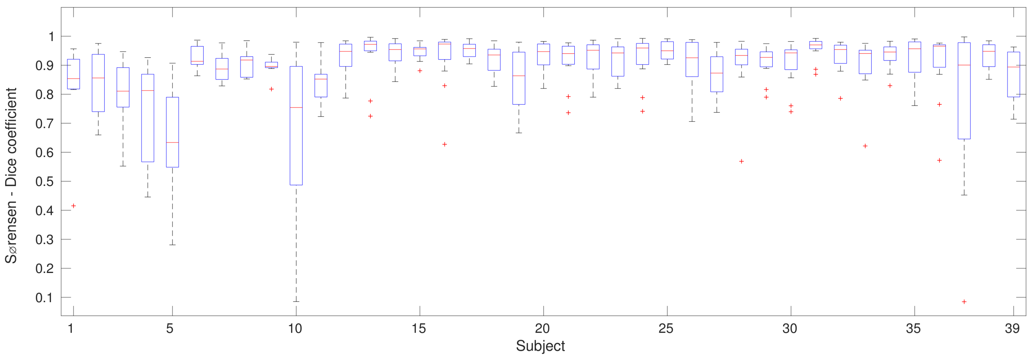
3.2. Segmentation Results

The results of the segmentation of all subjects can be seen in Figure 7. All informative segments were detected. Although several detections cover only a small part, the majority of the detections is accurate with an average SDC of 0.8932 (std 0.1202). However, the distribution is highly skewed since 94.81% of the segments obtained an SDC higher than 0.7.

The SDC’s calculation only takes into account correctly identified segments, that is, overlapping with the given segments for informative activities. However, non-informative segments have been detected as well, segments where activity occurs that should be rejected. On average 55.61 additional segments were found, with a maximum of 87. The next section discusses how well all of these can be discarded while still retaining the informative segments.

3.3. Combination Results

The number of false detections, the percentage of correct detections and the accuracies, with and without taking into account the formers, are given in

Table 3. Results for the combination of segmentation and classification expressed with the number of false detections (FD), the Detection True Positive Rate (DTPR), the pure accuracy (ACC${}_p$) and the actual accuracy (ACC${}_a$) using HODA and simple features.

	HODA				Simple
Subject	FD	DTPR	ACC${}_{\mathit{p}}$ (%)	ACC${}_{\mathit{a}}$ (%)	FD	DTPR	ACC${}_{\mathit{p}}$ (%)	ACC${}_{\mathit{a}}$ (%)
1	3	0.5	50	18.1818	9	0.25	50	5.8824
2	16	0.8750	71.4286	20.8333	15	0.625	60	13.0435
3	8	0.8750	85.7143	37.5	12	0.875	100	35
4	5	0.6250	80	30.7692	7	0.625	80	26.6667
5	6	0.7500	33.3333	14.2857	12	0.5	0	0
6	10	0.8750	85.7143	33.3333	19	0.875	71.4286	18.5185
7	3	1	75	54.5455	8	0.75	100	37.5
8	5	0.7500	66.6667	30.7692	6	1	87.5	50
9	5	0.7500	100	46.1538	15	0.75	83.3333	21.7391
10	4	0.5	100	33.3333	13	0.625	80	19.0476
11	7	0.6250	80	26.6667	10	1	37.5	16.6667
12	3	0.9167	81.8182	60	10	0.75	100	40.9091
13	0	0.5	100	50	7	0.9167	81.8182	47.3684
14	2	0.8333	90	64.2857	7	0.8333	100	52.6316
15	2	1	75	64.2857	6	0.8333	100	55.5556
16	3	0.8333	80	53.3333	5	0.8333	100	58.8235
17	2	0.9167	90.9091	71.4286	15	0.9167	81.8182	33.3333
18	0	1	91.6667	91.6667	2	1	83.3333	71.4286
19	0	1	91.6667	91.6667	6	0.8333	100	55.5556
20	1	1	100	92.3077	4	0.9167	81.8182	56.2500
21	0	1	83.3333	83.3333	1	0.8333	100	76.9231
22	6	0.8333	90	50	21	0.6667	87.5	21.2121
23	2	1	83.3333	71.4286	6	0.75	100	50
24	0	0.8333	100	83.3333	0	0.75	100	75
25	0	0.8333	100	83.3333	4	1	83.3333	62.5
26	2	1	91.6667	78.5714	4	1	75	56.25
27	0	1	100	100	1	1	91.6667	84.6154
28	1	0.9167	81.8182	69.2308	10	0.75	55.5556	22.7273
29	0	0.9167	100	91.6667	6	0.8333	100	55.5556
30	0	1	100	100	3	1	91.6667	73.3333
31	2	0.6667	100	57.1429	6	0.7500	100	50
32	2	1	91.6667	78.5714	9	0.9167	90.9091	47.619
33	2	0.9167	90.9091	71.4286	7	0.8333	90	47.3684
34	1	0.8333	100	76.9231	8	1	91.6667	55
35	2	1	83.3333	71.4286	5	0.8333	70	41.1765
36	1	0.8333	80	61.5385	8	0.9167	81.8182	45
37	6	0.5833	85.7143	33.3333	10	0.5833	71.4286	22.7273
38	0	1	100	100	8	0.9167	90.9091	50
39	1	1	91.6667	84.6154	3	1	83.3333	66.6667
AVG	2.8974	0.8536	86.7272	62.3391	7.8974	0.8216	82.9061	44.0922
STD	3.3150	0.1576	14.2076	25.0301	4.7395	0.1630	20.3669	20.7116

for both HODA and simple features.

The number of false positives is decreased by applying the classifier. From the average 55.61, for HODA, only 2.90 remain, with a maximum of 16. Ten subjects correctly rejected all spurious activities. In contrast, the simple features still have an average of 7.90 false detections, with a maximum of 21 and only for a single subject, all false detections were rejected.

Rejection is a trade-off, balanced with the amount of correct detections. For HODA, on average, 85.36% of the segments are detected, but large differences between individuals occur. 14 subjects detect all segments, but four only detect less than 60% of them. Using the simple features, 82.16% of the features are detected. The sign test indicates a significant difference in the DTPR ($p=0.0436$).

The last two columns bring everything together. ACC${}_p$ is equivalent to the performance for the classification experiment performed in this study, but the detected segment boundaries are used, rather than the ideal ones. Moreover, non-detected segments are dropped. As a consequence, for HODA, classification accuracy drops on average from 94.34 to 86.72%. Subject one only recognizes half of the activities and subject five only one third of them. In contrast, 12 subjects recognize all detected activities perfectly and nine more recognize more than or equal to 90% correctly. The result for the simple features improves from 78.21 to 82.91%. This signifies that the segments that were rejected could not be recognized easily and were wrongly classified even if segmented perfectly. Despite this increase, HODA outperforms the simple features significantly ($p=0.0326$).

The last column shows the combined effects of the previous three columns and represent the complete performance of the system. For HODA, it drops with 24% to an average of 62.34%. As a general system, this is insufficient. Yet, for some subjects, the performance is much better. The low performance is due to several badly-predicted subjects. 13 have an accuracy below or equal to 50%. On the other side of the scale, 11 perform better than 70% and four above 90%. Three subjects achieved perfect detection and recognition, yielding a global performance of 100%. The performance difference with the simple features is immediately apparent and highly significant ($p<0.01$). The large difference might seem surprising given the previous two columns with much smaller differences, but it can be explained by the high number of false positives. As an example, subject 38 has 12 target occurrences of activities. The simple features approach detects 11 of them. Ten out of these 11 are classified correctly. However, eight false positives are considered as wrongly classified, leading to an actual accuracy of 50%.

Finally, performance can be grouped by activity rather than by subject.

Table 4. Performance for the combined segmentation and classification, grouped by activity, expressed as the Detection True Positive Rate (DTPR), the pure accuracy (ACC${}_p$) and the actual accuracy (ACC${}_a$) using HODA features.

	DTPR	ACC${}_{\mathit{p}}$ (%)	ACC${}_{\mathit{a}}$ (%)
getUp	0.9103	95.7746	87.1795
lieDown	0.875	100	87.5
maxReach	1	100	100
pen5	0.8718	79.4118	69.2308
reach5	0.7436	93.1034	69.2308
sts5	0.8333	66.1538	55.1282

gives an overview for the HODA features. The same trends as in the confusion matrix in Table 2 can be observed. The non-repetitive activities perform better. This might be due to the fact they resemble often-occurring activities such as walking. Overall, the problem is mostly with sts5 which has an actual recognition performance of only 55.13%.

4. Discussion

The results show that the newly proposed activity recognition approach with HODA outperforms a more standard direct comparison based on the distances derived from dynamic time warping, both in a closed world scenario and in the inclusion of false and missed detections. The significant improvement is due to taking into account the entire signals, not only the reduced similarity information. Of course, it should be noted that the final feature space with HODA offers more degrees of freedom for the classifier since it is generally of higher dimensionality, around 30. Nevertheless, this is not only an advantage because it also increases the danger of overfitting.

It is also apparent that large differences between subjects exist. As an example, Table 3 shows performances ranging from 18 to 100%. This shows that the effectiveness of the model greatly depends on the subject. In this study, training was performed in a leave-one-subject-out approach. Hence, a subject-independent model was produced. As an alternative, data from the subject to be tested could either be part of the training set or only subject-specific data could be used. A model constructed in this way is expected to perform better for a specific subject, but it is less generally applicable.

Another factor influencing the performance is the manual labelling of the data. It is not exhaustive, so some false detections might actually be correct. These detections have not been checked manually afterwards. Moreover, in this case, correct segments would have ended up in the set of examples for rejection, leading to a less discriminative choice of features.

The performance is also determined by the choice of approach and features. The methods employed in this study heavily rely on pattern matching, based on the hypothesis that the acceleration pattern captures the entire activity. As much relevant variability as possible was captured through DTW and HODA-derived subspaces. Nevertheless, patterns also contain inherent noise in the sense that parts of the movement are not defining aspects of a particular activity. Current results are promising for many subjects, but an earlier study on the Sensewear dataset showed that much is to be gained by combining pattern features with more general statistical features [47]. In the future, it could be beneficial to merge the feature set obtained by HODA with the statistical features employed there. This is especially true for segmentation. The recognition results based on ideal segments are very good, but due to falsely rejected or only partly covered segments this performance drops in the final result.

Looking more in detail at the results in Table 3 reveals a recurring issue. The data description mentioned that two datasets were merged to increase population size and strengthen the conclusions. In the analyses, the first 11 subjects belong to the most recent data acquisition with the Shimmer, whereas the last 28 are recorded with the Sensewear Armband. In all recognition experiments, the Sensewear set outperforms the Shimmer, both with the HODA and the simple features. For the HODA features in the closed world scenario, the performance difference amounts to 10%. Also, in segmentation, the difference between the datasets is noticeable. The 11 Shimmer subjects seem to have been segmented less accurately, e.g., subject five and ten. This might be because the segmentation becomes more difficult if the activities under consideration are executed in a shorter time span without interruption or with immediate displacements afterwards. Ideally, the signal would be static in between activities and the activities themselves would be executed fluidly, without pauses. In (emulated) real-life settings, these ideal conditions are not always fulfilled. Finally, in the overall performance measure ACC${}_a$, the gap grows to more than 40% due to worse rejection and recognition. With the simple features, both datasets perform worse and the difference between them increases further. The results lead to the conclusion that HODA, apart from performing better, also succeeds in shrinking the performance gap between the two datasets.

Several explanations can be mentioned: more activities are taken from the Sensewear set and segmentation seems more successful due to more standardized behaviour, e.g., pauses in between activities. A more important issue is likely the sensor itself. The Sensewear is an armband with a built-in strap, meaning that its positioning with respect to the arm is more likely to be similar between subjects. The Shimmer has to be attached manually. Moreover, it contains three axes instead of two. Although care has been taken to attach the sensor and select the axes corresponding to the Sensewear, no further correction other than normalization with respect to the magnitude of gravity was applied to harmonize the two datasets. Many calibration parameters could introduce small differences. The performance difference is hence likely caused by three effects: differences within the Shimmer dataset are larger due to sensor setup, there are differences between the datasets and the Sensewear data has more influence in the training process due to its higher number of subjects. In further studies, it would therefore be advised to use the same sensor for all recordings. This did not happen here because the Sensewear was no longer available. Also, a future study could compare the sensors more explicitly, which was not the aim here. In this study, data from both sets contribute to the classifier and influence the results. In itself, this shows that HODA can obtain good results and is more robust against the heterogeneity than simple DTW features. Yet, performing the identical study on two separate sets of the same size with the different sensors might further clarify the impact of the sensor type.

The most important drawback of the algorithm is its high computational cost. If more activities would be considered, it would even be higher. Training can be done in advance, but testing alone is also costly. In its current state, it is not suitable for real-time use. Structuring the data and applying HODA is not computationally expensive. The repeated application of DTW proves to be the biggest concern. It could be alleviated by using existing dedicated hardware. However, in the context of assessment of functional capacity, computational cost is not an issue. Current practice consists of a weekly BASFI assessment. Disease evolution over time could be tracked in more detail by a daily automatic assessment, which can be reported to the clinician when available. This could detect fluctuations during the week, but also between weekly meetings. Real-time recognition could be useful e.g., to detect and correct maladaptive poses through direct feedback, which is another possible aim. In that case, another approach is preferable.

The study is part of a larger aim for assessment of functional capacity by objective means. For this reason, the data was acquired from axSpA patients rather than healthy subjects. As mentioned in the introduction, patient data is more difficult to classify. The study shows that HODA features, exploiting the structure in the data, outperform simple pattern features in this difficult setting.

Furthermore, it addresses the problem of the limited applicability of pattern detection compared to sliding window approaches. This is achieved through the approach to rejection, first looking for dynamic segments and then rejecting non-informative segments as rejection class. The reason for rejection can be three-fold. Firstly, the rejection class serves as a model. If similar non-informative segments are segmented, they can be rejected. Secondly, some segments are only partly segmented, which diminishes their resemblance to the class pattern. Hence, they are rejected by the final classifier. Thirdly, some activities are badly recognized to begin with, even when ideally segmented. This might lead to them resembling the collection of rejection segments rather than their own class. This shows that, through segmentation, the continuous problem can be converted into a discrete one. Subsequently, the same approach as with sliding windows can be implemented, making the rejection class part of a multi-class problem. The current approach has the advantage to explicitly aim for meaningful segments, whereas this is not guaranteed with basic windowing.

The setup of the protocol, together with the less limited applicability make it possible to have patients potentially record themselves in the home environment. Using a single sensor makes it easy to set up. Moreover, because only accelerometry is needed, the sensor will suffer less from power restrictions.

A next step would try to extract activity characteristics related to the functional capacity. A typical example already used in practice is activity duration. In this regard, the low number of false detections for the majority of subjects is a key strength. False detections would introduce meaningless assessment characteristics. A lower detection rate is less important as long as enough data is available to still assess the functionality. As a results, the current algorithm can be considered a building block for further research.

5. Conclusions

This paper introduced an approach to segment and recognize six activities from single arm-worn accelerometer. Data segments are extracted based on the variance of the acceleration. They are represented as multiway data structures (tensors) containing pattern similarity derived with Dynamic Time Warping. Next, Higher Order Discriminant Analysis serves to extract subspaces for the classes, resulting in data features. A Random Forest with an additional rejection class finally classifies the data into one of the activity classes.

The setup was evaluated on a dataset of 39 axSpA patients and compared to a simpler direct DTW similarity approach. HODA segmentation and classification showed good performance individually, but their combination led only to good results for part of the subjects, in particular a subset of the data that was recorded with another device. The evaluation shows the viability of the approach which significantly outperforms the benchmark’s performance. For future work, statistical features could be included to improve performance, particularly for rejection.

References

1. O’Dwyer, T.; O’Shea, F.; Wilson, F. Exercise therapy for spondyloarthritis: A systematic review. Rheumatol. Int. 2014, 34, 887–902. [Google Scholar] [CrossRef] [PubMed]
2. Rudwaleit, M.; van der Heijde, D.; Landewé, R.; Listing, J.; Akkoc, N.; Brandt, J.; Braun, J.; Chou, C.T.; Collantes-Estevez, E.; Dougados, M.; et al. The development of Assessment of SpondyloArthritis international Society classification criteria for axial spondyloarthritis (part II): Validation and final selection. Ann. Rheum. Dis. 2009, 68, 777–783. [Google Scholar] [CrossRef] [PubMed]
3. Calin, A.; Garrett, S.; Whitelock, H.; Kennedy, L.G.; O’Hea, J.; Mallorie, P.; Jenkinson, T. A new approach to defining functional ability in ankylosing spondylitis: The development of the Bath Ankylosing Spondylitis Functional Index. J. Rheumatol. 1994, 21, 2281–2285. [Google Scholar] [PubMed]
4. Weiss, A.; Herman, T.; Plotnik, M.; Brozgol, M.; Maidan, I.; Giladi, N.; Gurevich, T.; Hausdorff, J.M. Can an accelerometer enhance the utility of the Timed Up & Go Test when evaluating patients with Parkinson’s disease? Med. Eng. Phys. 2010, 32, 119–125. [Google Scholar] [CrossRef] [PubMed]
5. Swinnen, T.W.; Milosevic, M.; Van Huffel, S.; Dankaerts, W.; Westhovens, R.; de Vlam, K. Instrumented BASFI (iBASFI) Shows Promising Reliability and Validity in the Assessment of Activity Limitations in Axial Spondyloarthritis. J. Rheumatol. 2016, 43, 1532–1540. [Google Scholar] [CrossRef] [PubMed]
6. Aggarwal, J.; Cai, Q. Human Motion Analysis: A Review. Comput. Vis. Image Underst. 1999, 73, 428–440. [Google Scholar] [CrossRef]
7. Poppe, R. A survey on vision-based human action recognition. Image Vis. Comput. 2010, 28, 976–990. [Google Scholar] [CrossRef]
8. Williamson, J.; Liu, Q.; Lu, F.; Mohrman, W.; Li, K.; Dick, R.; Shang, L. Data sensing and analysis: Challenges for wearables. In Proceedings of the 20th Asia and South Pacific Design Automation Conference, Chiba, Japan, 19–22 January 2015; pp. 136–141. [Google Scholar]
9. Roetenberg, D.; Luinge, H.; Slycke, P. Xsens MVN: Full 6DOF Human Motion Tracking Using Miniature Inertial Sensors; Technical Report; Xsens: Enschede, The Netherlands, 2009. [Google Scholar]
10. Altini, M.; Penders, J.; Vullers, R.; Amft, O. Estimating Energy Expenditure Using Body-Worn Accelerometers: A Comparison of Methods, Sensors Number and Positioning. IEEE J. Biomed. Health Inform. 2015, 19, 219–226. [Google Scholar] [CrossRef] [PubMed]
11. Bouten, C.; Westerterp, K.; Verduin, M.; Janssen, J. Assessment of energy expenditure for physical activity using a triaxial accelerometer. Med. Sci. Sports Exerc. 1994, 23, 21–27. [Google Scholar] [CrossRef]
12. Lyden, K.; Kozey, S.L.; Staudenmeyer, J.W.; Freedson, P.S. A comprehensive evaluation of commonly used accelerometer energy expenditure and MET prediction equations. Eur. J. Appl. Physiol. 2011, 111, 187–201. [Google Scholar] [CrossRef] [PubMed]
13. Crouter, S.E.; Churilla, J.R.; Bassett, D.R. Estimating energy expenditure using accelerometers. Eur. J. Appl. Physiol. 2006, 98, 601–612. [Google Scholar] [CrossRef] [PubMed]
14. Kozey-Keadle, S.; Libertine, A.; Lyden, K.; Staudenmayer, J.; Freedson, P.S. Validation of wearable monitors for assessing sedentary behavior. Med. Sci. Sports Exerc. 2011, 43, 1561–1567. [Google Scholar] [CrossRef] [PubMed]
15. Butte, N.F.; Ekelund, U.; Westerterp, K.R. Assessing physical activity using wearable monitors: Measures of physical activity. Med. Sci. Sports Exerc. 2012, 44, S5–S12. [Google Scholar] [CrossRef] [PubMed]
16. Maurer, U.; Smailagic, A.; Siewiorek, D.; Deisher, M. Activity recognition and monitoring using multiple sensors on different body positions. In Proceedings of the 2006 BSN International Workshop on Wearable and Implantable Body Sensor Networks, Cambridge, MA, USA, 3–5 April 2006; pp. 113–116. [Google Scholar]
17. Preece, S.; Goulermas, J.; Kenney, L.; Howard, D.; Meijer, K.; Crompton, R. Activity identification using body-mounted sensors—A review of classification techniques. Physiol. Meas. 2009, 30, R1–R33. [Google Scholar] [CrossRef] [PubMed]
18. Bulling, A.; Blanke, U.; Schiele, B. A Tutorial on Human Activity Recognition Using Body-worn Inertial Sensors. ACM Comput. Surv. 2014, 46, 33:1–33:33. [Google Scholar] [CrossRef]
19. Lara, O.D.; Labrador, M.A. A survey on human activity recognition using wearable sensors. IEEE Commun. Surv. Tutor. 2013, 15, 1192–1209. [Google Scholar] [CrossRef]
20. Chavarriaga, R.; Sagha, H.; Calatroni, A.; Digumarti, S.T.; Tröster, G.; del R. Millán, J.; Roggen, D. The Opportunity challenge: A benchmark database for on-body sensor-based activity recognition. Pattern Recognit. Lett. 2013, 34, 2033–2042. [Google Scholar] [CrossRef]
21. Preece, S.; Goulermas, J.; Kenney, L.; Howard, D. A Comparison of Feature Extraction Methods for the Classification of Dynamic Activities From Accelerometer Data. IEEE Trans. Biomed. Eng. 2009, 56, 871–879. [Google Scholar] [CrossRef] [PubMed]
22. Avci, A.; Bosch, S.; Marin-Perianu, M.; Marin-Perianu, R.; Havinga, P. Activity recognition using inertial sensing for healthcare, wellbeing and sports applications: A survey. In Proceedings of the 2010 23rd International Conference on Architecture of Computing Systems (ARCS), Hannover, Germany, 22–23 February 2010; pp. 1–10. [Google Scholar]
23. Altun, K.; Barshan, B. Human Activity Recognition Using Inertial/Magnetic Sensor Units; Human Behavior Understanding; Salah, A.A., Gevers, T., Sebe, N., Vinciarelli, A., Eds.; Springer: Berlin/Heidelberg, Germany, 2010; pp. 38–51. [Google Scholar]
24. Leutheuser, H.; Schuldhaus, D.; Eskofier, B.M. Hierarchical, Multi-Sensor Based Classification of Daily Life Activities: Comparison with State-of-the-Art Algorithms Using a Benchmark Dataset. PLoS ONE 2013, 8, e75196. [Google Scholar] [CrossRef] [PubMed]
25. Bao, L.; Intille, S.S. Activity Recognition from User-Annotated Acceleration Data; Pervasive Computing; Ferscha, A., Mattern, F., Eds.; Springer: Berlin/Heidelberg, Germany, 2004; pp. 1–17. [Google Scholar]
26. Casale, P.; Pujol, O.; Radeva, P. Human Activity Recognition from Accelerometer Data Using a Wearable Device. In Pattern Recognition and Image Analysis; Vitrià, J., Sanches, J.M., Hernández, M., Eds.; Springer: Berlin/Heidelberg, Germany, 2011; pp. 289–296. [Google Scholar]
27. Mannini, A.; Intille, S.S.; Rosenberger, M.; Sabatini, A.M.; Haskell, W. Activity recognition using a single accelerometer placed at the wrist or ankle. Med. Sci. Sports Exerc. 2013, 45, 2193. [Google Scholar] [CrossRef] [PubMed]
28. Banos, O.; Galvez, J.M.; Damas, M.; Pomares, H.; Rojas, I. Window size impact in human activity recognition. Sensors 2014, 14, 6474–6499. [Google Scholar] [CrossRef] [PubMed]
29. Khan, A.M.; Lee, Y.K.; Lee, S.Y.; Kim, T.S. A triaxial accelerometer-based physical-activity recognition via augmented-signal features and a hierarchical recognizer. IEEE Trans. Inf. Technol. Biomed. 2010, 14, 1166–1172. [Google Scholar] [CrossRef] [PubMed]
30. Ganea, R.; Paraschiv-lonescu, A.; Aminian, K. Detection and Classification of Postural Transitions in Real-World Conditions. IEEE Trans. Neural Syst. Rehabilit. Eng. 2012, 20, 688–696. [Google Scholar] [CrossRef] [PubMed]
31. Albert, M.V.; Toledo, S.; Shapiro, M.; Koerding, K. Using mobile phones for activity recognition in Parkinson’s patients. Front. Neurol. 2012, 3, 158. [Google Scholar] [CrossRef] [PubMed]
32. Huisinga, J.M.; Mancini, M.; St. George, R.J.; Horak, F.B. Accelerometry Reveals Differences in Gait Variability Between Patients with Multiple Sclerosis and Healthy Controls. Ann. Biomed. Eng. 2012, 41, 1670–1679. [Google Scholar] [CrossRef] [PubMed]
33. Muscillo, R.; Conforto, S.; Schmid, M.; Caselli, P.; D’Alessio, T. Classification of Motor Activities through Derivative Dynamic Time Warping applied on Accelerometer Data. In Proceedings of the 29th Annual International Conference of the IEEE Engineering in Medicine and Biology Society (EMBS), Lyon, France, 23–26 August 2007; pp. 4930–4933. [Google Scholar]
34. Margarito, J.; Helaoui, R.; Bianchi, A.M.; Sartor, F.; Bonomi, A.G. User-Independent Recognition of Sports Activities From a Single Wrist-Worn Accelerometer: A Template-Matching-Based Approach. IEEE Trans. Biomed. Eng. 2016, 63, 788–796. [Google Scholar] [CrossRef] [PubMed]
35. Zhang, M.; Sawchuk, A.A. Motion Primitive-based Human Activity Recognition Using a Bag-of-features Approach. In Proceedings of the 2nd ACM SIGHIT International Health Informatics Symposium, Miami, FL, USA, 28–30 January 2012; pp. 631–640. [Google Scholar]
36. Lee, Y.S.; Cho, S.B. Activity recognition using hierarchical hidden markov models on a smartphone with 3D accelerometer. In Proceedings of the International Conference on Hybrid Artificial Intelligence Systems, Wroclaw, Poland, 23–25 May 2011; Springer: Berlin/Heidelberg, Germany, 2011; pp. 460–467. [Google Scholar]
37. Guenterberg, E.; Ostadabbas, S.; Ghasemzadeh, H.; Jafari, R. An Automatic Segmentation Technique in Body Sensor Networks Based on Signal Energy. In Proceedings of the BodyNets ’09 Fourth International Conference on Body Area Networks, Los Angeles, CA, USA, 1–3 April 2009; ICST (Institute for Computer Sciences, Social-Informatics and Telecommunications Engineering): Brussels, Belgium, 2009; pp. 21:1–21:7. [Google Scholar]
38. Yang, A.Y.; Iyengar, S.; Kuryloski, P.; Jafari, R. Distributed segmentation and classification of human actions using a wearable motion sensor network. In Proceedings of the 2008 IEEE Computer Society Conference on Computer Vision and Pattern Recognition Workshops, Anchorage, AK, USA, 23–28 June 2008; pp. 1–8. [Google Scholar]
39. Phan, A.H.; Cichocki, A. Tensor decompositions for feature extraction and classification of high dimensional datasets. Nonlinear Theory Appl. IEICE 2010, 1, 37–68. [Google Scholar] [CrossRef]
40. Sieper, J.; Rudwaleit, M.; Baraliakos, X.; Brandt, J.; Braun, J.; Burgos-Vargas, R.; Dougados, M.; Hermann, K.; Landewe, R.; Maksymowych, W.; et al. The Assessment of SpondyloArthritis international Society (ASAS) handbook: a guide to assess spondyloarthritis. Ann. Rheum. Dis. 2009, 68, ii1–ii44. [Google Scholar] [CrossRef] [PubMed]
41. Müller, M. Dynamic Time Warping. In Information Retrieval for Music and Motion; Springer: Berlin/Heidelberg, Germnay, 2007; pp. 69–84. [Google Scholar]
42. Keogh, E.J.; Pazzani, M.J. Derivative dynamic time warping. In Proceedings of the 2001 SIAM International Conference on Data Mining, Chicago, IL, USA, 5–7 April 2001; pp. 1–11. [Google Scholar]
43. Zhou, F.; De la Torre, F. Generalized time warping for multi-modal alignment of human motion. In Proceedings of the 2012 IEEE Conference on Computer Vision and Pattern Recognition (CVPR), Providence, RI, USA, 16–21 June 2012; pp. 1282–1289. [Google Scholar]
44. Cichocki, A.; Mandic, D.; De Lathauwer, L.; Zhou, G.; Zhao, Q.; Caiafa, C.; Phan, H.A. Tensor decompositions for signal processing applications: From two-way to multiway component analysis. IEEE Signal Process. Mag. 2015, 32, 145–163. [Google Scholar] [CrossRef]
45. Phan, A.H. NFEA: Tensor Toolbox for Feature Extraction and Applications; Technical Report; Lab for Advanced Brain Signal Processing, Brain Science Institute RIKEN: Hirosawa Wako City, Japan, 2011. [Google Scholar]
46. Bader, B.W.; Kolda, T.G.; Sun, J.; Acar, E.; Dunlavy, D.M.; Chi, E.C.; Mayo, J. MATLAB Tensor Toolbox Version 3.0-Dev. 2017. Available online: https://www.tensortoolbox.org (accessed on 11 April 2018).
47. Billiet, L.; Swinnen, T.W.; Westhovens, R.; de Vlam, K.; Van Huffel, S. Accelerometry-Based Activity Recognition and Assessment in Rheumatic and Musculoskeletal Diseases. Sensors 2016, 16, 2151. [Google Scholar] [CrossRef] [PubMed]
48. Ho, T.K. Random decision forests. In Proceedings of the 3rd International Conference on Document Analysis and Recognition, Montreal, QC, Canada, 14–16 August 1995; Volume 1, pp. 278–282. [Google Scholar]
49. Izenman, A.J. Linear Discriminant Analysis. In Modern Multivariate Statistical Techniques: Regression, Classification, and Manifold Learning; Springer: New York, NY, USA, 2008; pp. 237–280. [Google Scholar]
50. Sørensen, T. A Method of Establishing Groups of Equal Amplitude in Plant Sociology Based on Similarity of Species Content and Its Application to Analyses of the Vegetation on Danish Commons; Biologiske Skrifter//Det Kongelige Danske Videnskabernes Selskab; I kommission Hos E. Munksgaard: København, Danmark, 1948. [Google Scholar]
Figure 1. Overview of the data representation. First, dynamic time warping (DTW) is used on sets of activity training segments to create activity patterns for all activities mentioned in Table 1. Next, a new data segment is matched on these patterns with DTW. Finally, the deformed representations are resampled and grouped in a tensor as a new multiway representation of the data segment. In this ideal case depicted here, the match is perfect for the correct class and random noise for the other classes.
Informatics 05 00020 g001
Figure 2. An illustration of Dynamic Time Warping. The full curve is warped to match the dashed curve according to the arrows.
Informatics 05 00020 g002
Figure 3. Illustration of a Tucker decomposition [45]. A tensor Y can be decomposed as a core tensor G and factor matrices A, B and C, one for each mode.
Informatics 05 00020 g003
Figure 4. Graphical summary of the HODA procedure. An ( N + 1 ) -way tensor is obtained by stacking the N-way training tensors. The orthogonal Tucker decomposition maximizing Fisher’s ratio yields the factor matrices A and core N-way core tensors G ( k ) vectorized as training features. Applying the factor matrices on test data similarly yields the test features [45].
Informatics 05 00020 g004
Figure 5. Classification accuracy for each subject using HODA features.
Informatics 05 00020 g005
Figure 6. A comparison of the classification accuracy using LDA on simple and HODA features.
Informatics 05 00020 g006
Figure 7. Segmentation performance for all subjects expressed as boxplots of individual Sørensen-Dice Coefficients (SDC) of the segments. All informative segments were detected.
Informatics 05 00020 g007