Abstract
Hard disk failure prediction is an important proactive maintenance method for storage systems. Recent years have seen significant progress in hard disk failure prediction using high-quality SMART datasets. However, in industrial applications, data loss often occurs during SMART data collection, transmission, and storage. Existing machine learning-based hard disk failure prediction models perform poorly on low-quality datasets. Therefore, this paper proposes a hard disk fault prediction technique based on low-quality datasets. Firstly, based on the original Backblaze dataset, we construct a low-quality dataset, Backblaze-, by simulating sector damage in actual scenarios and deleting 10% to 99% of the data. Time series features like the Absolute Sum of First Difference (ASFD) were introduced to amplify the differences between positive and negative samples and reduce the sensitivity of the model to SMART data loss. Considering the impact of different quality datasets on time window selection, we propose a time window selection formula that selects different time windows based on the proportion of data loss. It is found that the poorer the dataset quality, the longer the time window selection should be. The proposed model achieves a True Positive Rate (TPR) of 99.46%, AUC of 0.9971, and F1 score of 0.9871, with a False Positive Rate (FPR) under 0.04%, even with 80% data loss, maintaining performance close to that on the original dataset.
1. Introduction
Today, hard disks are the primary storage devices in computers, and many data centers rely on numerous hard disks to store critical information. In scenarios involving large-scale storage systems, such as high-performance computing and internet services [1], hard disk failures occur quite frequently. According to a survey in the literature [2], 78% of hardware replacements are due to hard disk failures. The catastrophic consequences of hard disk failures are permanent and difficult to recover from, thereby reducing the reliability of data centers. Therefore, predicting disk failures early not only reduces the risk of data loss but also lowers the cost of data recovery.
Hard disk failure prediction is an important proactive maintenance method for storage systems. Unlike traditional software operation and maintenance, which involves repairing faults after they occur, hard disk fault prediction is a passive process where operation and maintenance tools proactively handle potential system failures before they occur, in order to avoid data loss.
In the fields of internal combustion engine fault diagnostics and software vulnerability prediction, A. Srinivaas reviewed the methods of internal combustion engine fault detection, including model-based and data-driven approaches [3]. The fault prediction methods that combine advanced deep learning techniques, such as Transformer, have shown better performance in fault detection compared to traditional machine learning methods. Zhang B et al. [4] introduced a vulnerability prediction method based on multi-level N-gram feature extraction and heterogeneous ensemble learning. Considering the poor generalization performance and tendency to overfit of individual classifiers, the method combines the four best-performing classifiers as the base classifiers. The above methods all take into account the impact of features on prediction results, which is also applicable to hard disk failure prediction problems.
In practical industrial applications, the collection, transmission, and storage of hard disk SMART data can result in partial data loss due to various objective or subjective reasons. For instance, during data collection, various errors such as sensor errors, data transmission errors, and device failures may occur, leading to inaccurate or incomplete data within the dataset. Additionally, in large-scale data centers, SMART data collection may need to be disabled during holidays, which can result in missing SMART data during the shutdown period. Furthermore, maintenance engineers might intentionally corrupt sample data to reduce the accuracy of hard disk failure prediction technologies, aiming to prevent being replaced by intelligent operation and maintenance software. In the above situations, inaccurate or incomplete hard disk data, namely low-quality hard disk data, has been generated, which has a huge impact on accurately predicting hard disk failures. In this scenario, it is difficult to use high-quality datasets for fault prediction. If we can process low-quality datasets to make their prediction results close to those of high-quality datasets, it will have great practical significance. In addition, if we can process low-quality datasets to make their prediction performance close to that of high-quality datasets, and even achieve good prediction performance even when 99% of data is lost, we can compress hard disk data in this way, greatly saving storage space and costs.
To address this, this paper proposes DFPoLD: A hard Disk Failure Prediction on Low-quality Datasets. The main contributions of this paper are as follows:
- (1)
- This paper constructs and open-sources a low-quality SMART dataset named Backblaze-. We first delete 10–99% of the 2022 data to create Backblaze-. Subsequently, we extract data, reset labels, select features, fill missing values, add time series features, and split the data into training and testing sets. Given the imbalance between positive and negative samples in hard disk datasets, we set the class_weight parameter during training to balance sample distribution. Additionally, we use stratified sampling when dividing the dataset, ensuring proportional representation of positive and negative samples in both training and testing sets.
- (2)
- For each SMART attribute, we constructed time series statistical features such as the Absolute Sum of First Difference (ASFDs) to reflect the absolute fluctuations between adjacent observations of the SMART data. Experimental results indicate that the introduction of time series features improves the accuracy of the model and enables earlier prediction of hard disk failures.
- (3)
- This paper fully considers the impact of different quality datasets on time window selection. By selecting a time window of 30 days and observing the changes in the predicted probability of hard disk failure over time, it is found that the quality of the dataset can affect the selection of time windows. We proposed a time window selection formula based on the proportion of hard disk data loss by fitting on datasets with 10%, 50%, and 80% data loss. The experimental results indicate that the poorer the quality of the dataset, the longer the time window selection should be. Choosing an appropriate time window can improve the accuracy of model prediction.
The reminder of this paper is organized as follows: Section 2 examines related research on hard drive failure prediction. Section 3 describes the construction process of low-quality datasets. We demonstrate the effectiveness of the Absolute Sum of First Difference (ASFD) and Complexity Invariant Distance (CID) time series features in Section 4. In Section 5,we use the LightGBM (LGB) model for prediction and the Optuna method for optimization. Section 6 verifies the effectiveness of the method. Finally, Section 7 summarizes the main findings.
2. Related Work
Over the past few decades, numerous scholars have proposed methods based on machine learning and deep learning to improve the accuracy of hard drive failure prediction:
These methods include using Long Short-Term Memory (LSTM) [5,6,7], Generative Adversarial Networks (GANs) [8], Regularized Greedy Forest (RGF) [9], Temporal Convolutional Networks (TCNs) [10], recurrent neural networks (RNNs) [11], and convolutional neural networks (CNNs) [12] to build hard disk failure prediction models. Unfortunately, these approaches are generally based on high-quality datasets for training, such as the Backblaze open-source dataset. Consequently, the applicability of these prediction models in scenarios involving low-quality datasets is limited.
Self-Monitoring Analysis and Reporting Technology (SMART) [13] can detect various operational metrics of hard disks, such as read/write counts, head load/unload cycles, and seek error rates. Traditional threshold-based hard disk failure prediction methods compare the current SMART attributes of the hard disk with preset thresholds. If the SMART attributes exceed the corresponding thresholds, the hard disk triggers an alert to the operating system. However, this approach only achieves a True Positive Rate (TPR) of 3% to 10% with a False Positive Rate (FPR) of 0.1%.Over the past few decades, many researchers have proposed various methods to improve the accuracy of failure prediction by using machine learning and deep learning techniques.
Alessio Burrello et al. [10] utilized Temporal Convolutional Networks (TCNs) for hard disk failure prediction. By leveraging real-world datasets, they found that TCNs outperformed Random Forest (RF) and Recurrent Neural Networks (RNNs), achieving approximately a 7.5% improvement in the Fault Detection Rate (FDR) and reducing the False Alarm Rate (FAR) to 0.052% within a 90-day input window. Alessio B. explored the architecture design space and proposed a range of models that offer various trade-offs between complexity, memory usage, and performance. Their results demonstrate that TCNs consistently outperform RNNs at any given model size and complexity.
Tianming J. approached hard drive failure prediction from the perspective of economic cost, aiming to minimize the cost of hard drive failure recovery [14]. They proposed the evaluation metric Mean-Cost-To-Recovery (MCTR) and employed a threshold-moving approach to find the optimal results. Evaluation on three real datasets demonstrated that compared to passive fault-tolerant techniques, MCTR reduced costs by 86.9%.
To address the poor performance of hard disk failure prediction in heterogeneous data centers, Ji Z. employed a twin neural network based on Long Short-Term Memory (LSTM) to obtain high-dimensional embedding vectors of hard disks [15]. By integrating a distance-based anomaly detection method, evaluations were conducted on both the Tencent and Backblaze datasets. Experimental results demonstrated that the use of mixed datasets combined with the anomaly detection method achieved better applicability and superior performance across datasets with different hard disk models, with AUC and F1 scores both exceeding 0.9. Compared to other models, this approach achieved the highest True Positive Rate (TPR) while maintaining a low False Positive Rate (FPR).
To enhance the prediction quality and timeliness of hard disk failure modeling, Han Wang proposed a two-layer classification-based feature selection scheme [16]. This method involves designing a filter to compute attribute importance, thereby filtering out attributes insensitive to failure recognition. Additionally, it determines feature correlations based on the correlation coefficient and introduces an attribute classification method. Experimental results show that this technique improves the prediction accuracy of ML/AI-based hard disk failure prediction models. Furthermore, under optimal conditions, the proposed scheme reduces training and prediction latency by 75% and 83%, respectively.
Mingyu Zhang proposed a novel failure prediction method based on the idea of blending ensemble learning on the publicly available Backblaze hard disk datasets [17]. Through the experimental results on multiple types of hard disks, an ensemble learning model with high performance on most types of hard disks is found, which solves the problem of the low robustness and generalization of traditional machine learning methods and proves the effectiveness and high universality of this method.
Wenqiang Ge proposed a new method for hard disk failure prediction to address the issue that the prediction performance for long-term failure and small-sample disks is not satisfactory [18]. The framework consists of a time-series feature extraction network and a prediction network. Experimental results on public datasets have demonstrated that our proposed method cannot only predict long-term failure but also has reliable prediction performance when facing small-sample disk data.
In summary, these methods have several main shortcomings:
- (1)
- Failure to consider the temporal aspect of hard drive data. Existing hard drive failure prediction methods mostly treat each day’s sampling of hard drive data as a single sample, neglecting the temporal information of the time series. Models typically only consider the state of the hard drive on a given day when making predictions. In hard drive failure prediction, a hard drive does not suddenly fail at a specific moment but undergoes a gradual deterioration process. Initially, the hard drive exhibits unstable parameters before eventually failing after a period of time. Therefore, capturing information during the period of unstable hard drive states can significantly improve prediction accuracy.
- (2)
- Lack of exploration of higher-order features. In hard drive failure prediction, most researchers use the raw SMART dataset for training. The raw SMART dataset includes both the raw and normalized values of SMART attributes, with each value being a number reported by the drive. However, the raw SMART dataset does not capture abrupt changes in the data. Therefore, incorporating higher-order time series features that can reflect sudden changes would improve the prediction model’s accuracy.
- (3)
- Poor applicability in industrial scenarios. Most existing research methods utilize high-quality datasets, such as the Backblaze open-source dataset. However, in real-world scenarios, the collected data often contains missing values and is generally of lower quality. Additionally, in practical applications, there is a significant imbalance between the number of positive and negative samples in the dataset. In performance evaluation experiments, current techniques typically randomly split the dataset into training and testing sets, which does not align with the actual application patterns in data centers.
Our previous work considered the temporal characteristics of hard disk data and constructed low-quality datasets [19]. In this study, we have made several significant optimizations:
- (1)
- The prior work did not account for the impact of dataset quality on time window selection, uniformly setting the time window to 10 days across datasets of varying quality, followed by data truncation and label resetting. In this study, we set the time window to 30 days and observed, across datasets of different qualities and using various models, that lower dataset quality necessitates a longer time window. This paper proposes a time window selection formula by setting a time window size of 1–30 days on datasets with 10%, 50%, and 80% data loss, and selecting the appropriate time window size based on the data loss ratio.
- (2)
- This study attempts to construct an extremely low-quality dataset by removing 99% of the data. Using this dataset, we trained the LGB model and compared its performance to datasets with 0% to 80% data loss. The results show decreases in both AUC score and F1 score, alongside a significant increase in FPR, with the rate of increase accelerating as more data is removed. Although TPR increases on this extremely low-quality dataset, the rapid rise in FPR indicates a higher misclassification rate. Thus, we conclude that higher dataset quality leads to a higher upper limit for hard disk failure prediction accuracy, while lower dataset quality reduces this upper limit.
- (3)
- The previous work did not take into account the probability of hard disks being predicted to fail over time. In this study, we observe the probability of hard disks being predicted as a failure over time in different models on low-quality datasets with 99% data loss and the datasets with 99% data loss and added ASFD features, by setting the time window to 30 days. Before adding ASFD time series features to the dataset, the probability of hard disks being predicted to be about to fail decreases over time. After adding features, the probability of failure prediction becomes flat over time, with a high prediction probability even before 30 days. This indicates that the ASFD time series features added in this paper increase the probability of the accurate prediction of the failure of hard disks, and offer advanced warning as to the time when hard disk failures are predicted. This further proves that ASFD is suitable for hard disk failure prediction scenarios.
3. Construction of Low-Quality Dataset
This article uses a dataset provided by Backblaze, a cloud storage service provider, from 1 January 2022 to 31 December 2023 [20]. The dataset is sampled once a day with no data loss, ensuring extremely high data quality. We select SMART data from the hard drives of the ST4000DM000 model provided by the S hard drive manufacturer as the initial dataset.
The initial dataset includes the following contents: (1) timestamp date, sampled daily; (2) hard disk serial number, serial_number; (3) hard disk model; (4) hard disk capacity, capacity_bytes; (5) label is_failure, where 0 indicates a healthy hard disk and 1 indicates a failed hard disk; and (6) SMART attributes. As shown in Table 1, the initial dataset comprises 36,849 hard disks, with 35,656 healthy disks and 1193 failed disks, resulting in a positive-to-negative sample ratio of 1:29. The number of positive samples in the dataset is significantly lower than that of negative samples. Therefore, to correct this imbalance, this paper sets the class_weight parameter to balance the sample quantities of different classes during model training. Additionally, when dividing the dataset, a stratified division principle is adopted, where positive and negative samples are separately divided into training and testing sets.

Table 1.
Initial dataset.
The data preprocessing process in this paper includes data truncation and label resetting, feature selection, random data deletion, and missing value imputation:
- (1)
- Data truncation and label resetting. Firstly, this paper truncates the data of hard disks in the initial dataset within a time window. Taking data from a single day of a hard disk might render the model unreliable, while using data from the entire lifespan of the disk could decrease the accuracy of the model. When selecting the size of the time window, this paper considers the effect of dataset quality on time window selection. We believe that the lower the quality of the dataset, the longer the time window should be extended to allow low-quality datasets to maintain a longer time window to reflect changes in feature trends. Through exploration, this paper proposes a time window selection formula that enables choosing an appropriate time window size based on the proportion of missing data in the dataset, as shown in Equation (1).
Here, x represents the proportion of missing data in the dataset (for example, if 50% of the data is missing, x is 0.5), and y represents the appropriate time window size to be set. We use the time window selection formula to choose an appropriate time window size y. Specifically, for failed hard disks, the paper selects the data from the last y days of the disk and labels this data as 1, indicating an imminent failure within the time window. As the initial dataset only assigns a label of 1 to failed disks on the day of failure, one of the key objectives of this paper is to predict whether a hard disk will fail within future time windows, necessitating the reassignment of labels for failed disks. For healthy disks, a different approach is employed for data truncation. Unlike the method used by Han S [21], this paper selects data from the first time window of y days for healthy disks and assigns a label of 0. This is because, within the first time window, the indicators of a healthy disk are the most stable and least prone to failure.
- (2)
- Feature selection. Features in the dataset that are all null or have zero variance are removed, as these features do not contribute to classification. The filtered features are shown in Table 2.
Table 2. SMART attributes after feature selection.
- (3)
- Random deletion of data. We simulate the situation of data loss caused by sector damage in actual scenarios and randomly delete SMART data. To prevent imbalanced sample distribution, we randomly delete the same proportion of data on positive and negative samples, i.e., delete 10~99% of the data, respectively, to construct a low-quality dataset Backblaze-. Our low-quality dataset has been open sourced (https://github.com/wwwwwst/Backblaze-.git (accessed on 17 January 2025)), including sixteen parts: all_data, drop_data_10, drop_data_20, drop_data_30, drop_data_40, drop_data_50, drop_data_60, drop_data_70, drop_data_80, drop_data_90, drop_data_91, drop_data_92, drop_data_93, drop_data_94, drop_data_95 and drop_data_99. The datasets are available at Open Science Framework (https://osf.io/6xd2a (accessed on 17 January 2025)) with a DOI of https://doi.org/10.17605/OSF.IO/6XD2A, and allocate license CC0 1.0 Universal.
- (4)
- Missing value imputation. In this study, missing values were imputed using the mode of the attribute column where the missing values occurred.
4. Time Series Features
As mentioned earlier, one limitation of current hard disk failure prediction methods is that the models only assess the status of the hard disk based on the SMART data from the same day. However, hard disk failures are gradual processes, and certain attribute values may exhibit abrupt changes before the failure occurs. Therefore, relying solely on the SMART data from a single day can lead to low model accuracy. In order to capture abrupt changes in attributes before a hard disk failure, we previously used Moving Average (MA) in our earlier work [22], but the results were not satisfactory. This paper employs a sliding window method to introduce time series features into the dataset. Specifically, the Absolute Sum of First Difference (ASFD) is primarily used, along with the Complexity Invariant Distance (CID) for comparison. These features, respectively, reflect the absolute fluctuations between consecutive SMART data observations and the complexity of time series data.
4.1. Absolute Sum of First Difference
The Absolute Sum of First Difference (ASFD) measures the changes or variations between values in a time series. It is calculated as the sum of the absolute differences between each element and its preceding element in a time series, as shown in Algorithm 1. For a given time series x = [1, 1, 0, 1, 0], the first differences are [0, 0, 1, 1, 1], and the ASFD is y = [0, 0, 1, 2, 3]. The ASFD result is a non-negative number, where a value of zero indicates that all values in the time series are identical, and higher values indicate greater changes between values.
| Algorithm 1 Calculate ASFD | |
| Input: Time Series x | |
| Output: y | |
| 1: | Initialization: y [0] = 0, n = x.length() |
| 2: | for i ← 1 to n − 1 do |
| 3: | y[i] = y[i − 1] + |x[i] − x[i − 1]| |
| 4: | return y |
This paper demonstrates the effectiveness of ASFD through the simulation of four time series:
- (1)
- A time series of length 100 with all values set to 0.
- (2)
- Based on time series 1, one point is randomly selected and set to 10.
- (3)
- Based on time series 1, one point is randomly selected and set to 100.
- (4)
- Based on time series 1, two points are randomly selected and set to 10.
As shown in Figure 1, the ASFD feature can effectively assess the absolute fluctuations between adjacent observations in a time series and detect abrupt changes within the series.
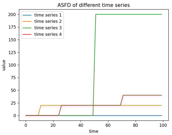
Figure 1.
ASFD of different time series.
- (1)
- Compared to a constant time series, the addition of abrupt changes increases the ASFD.
- (2)
- The more an abrupt value deviates from the normal value, the larger the ASFD of that time series.
- (3)
- The more frequent the abrupt changes, the larger the ASFD of that time series.
- (4)
- The ASFD magnitude accumulates with the number of abrupt changes.
4.2. Complexity Invariant Distance
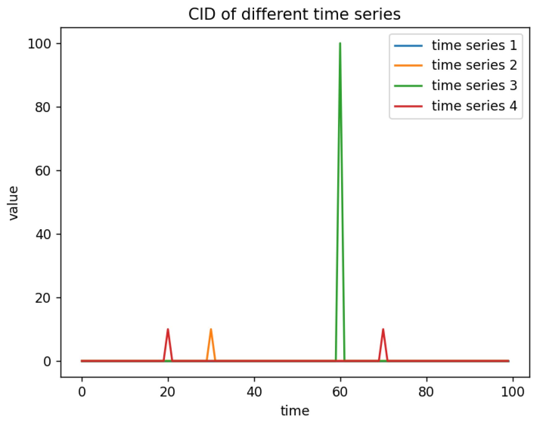
Complexity Invariant Distance (CID) is a measure used to compare the similarity between two time series (Q and C). It addresses the limitations of traditional distance metrics, such as Euclidean distance and Manhattan distance, in handling complex data distributions. To demonstrate the effectiveness of CID, the four time series simulated in Section 4.1 are used.
The experimental results, as shown in Figure 2, demonstrate that the CID feature effectively evaluates the complexity of time series as well as the occurrence of abrupt changes within them.

Figure 2.
CID of different time series.
- (1)
- Compared to a constant time series, the introduction of abrupt changes increases the CID value.
- (2)
- The more the value deviates from the normal value, the higher the CID of the time series.
- (3)
- The more frequent the abrupt changes, the greater the CID of the time series.
As mentioned earlier, the failure of a hard drive is a gradual process, and before the hard drive fails, some attribute values may undergo sudden changes. However, a sudden change does not mean that the hard drive will immediately fail, but rather, there is an accumulation process until a certain threshold is reached, at which point the hard drive will fail. In Section 4.1, we can observe that the ASFD size accumulates with the number of mutations, which is more in line with the characteristics of hard disk failures. The CID in Section 4.2 only reflects the occurrence of mutations. Meanwhile, in Experiment 6.5, it was demonstrated that ASFD improves the predictive performance of the model. In summary, ASFD outperforms CID.
5. Hard Disk Failure Prediction Model Based on Low-Quality Datasets
Considering that the quality of the dataset results in different time windows, we propose a time window selection formula to set an appropriate time window for truncation. Through the validation of the validity of time series in Section 4, we found that the time series features Absolute Sum of First Difference (ASFD) and Complexity Invariant Distance (CID) can be used to reflect the absolute fluctuations and time series complexity between adjacent observations of SMART data on hard disks. Therefore, we added the above two time series features to the preprocessed dataset in Section 3 and trained the model using LightGBM (LGB) [23], while Optuna optimized the model.
5.1. Hard Disk Failure Prediction Process
The hard disk failure prediction process in this paper mainly includes the following steps:
- (1)
- Adding Time Series Features. After preprocessing the initial 2022 dataset as described in Section 3, ASFD and CID features were added to each SMART attribute. The dataset used in this paper has a total of 121 features, including 41 SMART attributes, 41 ASFD features, and 39 CID features. Since features with zero variance are removed after generation, the number of CID features may not match the number of SMART features.
- (2)
- Splitting the Training and Testing Sets. The data was split into training and testing sets using a stratified approach, ensuring that both positive and negative samples were proportionally represented in each set. The data was randomly divided into 80% training and 20% testing sets.
- (3)
- Model Training. The LightGBM (LGB) model developed by Microsoft [22] was used to train the hard disk failure prediction model using the preprocessed training set. Additionally, other model algorithms were tested to compare their prediction accuracy.
- (4)
- Model Tuning. Optuna was used to find the optimal hyperparameters for the LightGBM algorithm, allowing for model tuning.
- (5)
- Hard Disk Failure Prediction. Once the optimal failure prediction model was obtained, the test set data was input into the model to obtain disk-level predictions, indicating whether each hard disk was likely to fail.
- (6)
- Model Evaluation. Using the disk-level predictions from the test set and the corresponding labels, the model’s performance was evaluated with AUC, F1 score, and TPR (where FPR < 0.1%).
- (7)
- Calculation of Days Predicted in Advance. After obtaining the trained high-performance model, the non-reset labeled data of all failed hard disks from 2023 was used as the test set to calculate the days the model predicted the failures in advance (DPF).
The pseudocode for the hard disk fault prediction process is shown in Algorithm 2:
| Algorithm 2 Hard Disk Failure Prediction | |
| Input: The pre-processed dataset, The failure_disk_2023 dataset | |
| Output: TPR, AUC, F1 score, DPF | |
| 1: | Initialization: N = SMART_attributes.length() |
| 2: | for n ← 0 to N do |
| 3: | add CID feature(each smart attr) |
| 4: | add ASFD feature(each smart attr) |
| 5: | Remove features with zero variance |
| 6: | Update dataset ← generate dataset |
| 7: | train_set,test_set = split_dataset(dataset) |
| 8: | lgb_model = LightGBM(), lgb_model.train(train_set) |
| 9: | Optimal_hyperparameters = optuna.optimize(lgb_model, param_space) |
| 10: | pre = lgb_model.predict(test_set) |
| 11: | failure_pre = lgb_model.predict(failure_disk_2023_dataset) |
| 12: | Update disk_pre ← map_func(pre, threshold) |
| 13: | Calculating Model Evaluation Metrics and DPF |
5.2. Model Hyperparameter Tuning
For hyperparameter tuning, many researchers use the brute-force GridSearch method [24,25,26]. While straightforward, it is notably time-consuming. In contrast, Bayesian framework-based tuning methods such as HyperOPT [27,28,29] and Optuna [30,31] are more efficient and powerful. Optuna, being lightweight and extremely fast, was chosen as the tuning method in this study.
Typically, the hyperparameters of tree-based models can be divided into four categories:
- (1)
- Parameters affecting the structure and learning of the decision tree.
- (2)
- Parameters influencing training speed.
- (3)
- Parameters improving accuracy.
- (4)
- Parameters preventing overfitting.
In most cases, there is significant overlap among these categories. Improving efficiency in one category may reduce efficiency in another. Relying solely on manual tuning is time-consuming, labor-intensive, and challenging to find the optimal balance. However, if an appropriate parameter grid is provided, Optuna can automatically search and identify the most balanced combination of parameters among these categories, thereby optimizing overall performance.
In Experiment 6.5, model comparison and experiments were conducted using the SMART+ASFD+CID dataset with 80% data loss to train the LGB model. After Optuna, the optimal hyperparameters of the LGB model are shown in Table 3.
Table 3.
Optimal hyperparameters of LGB model.
5.3. Time Window Setting
To improve the accuracy of the model’s predictions, we conducted experiments on time window selection, as detailed in Experiment 6.6. This paper considers that using data from only a single day of a hard drive’s life may make the model unreliable, while using data from the entire lifecycle may reduce the model’s accuracy. Therefore, a time window is applied to the dataset. Additionally, this paper thoroughly considers the impact of time window selection on hard drive failure prediction results, acknowledging that different time window settings on datasets of varying quality can affect the final prediction outcomes. To facilitate setting an appropriate time window based on dataset quality, this paper proposes a time window selection formula that allows selecting an optimal time window size according to the proportion of missing data in the dataset, as shown in Equation (1) in Section 3.
Using this time window selection formula to set an appropriate time window improves the accuracy for hard disk failures, achieving results on low-quality datasets that are very close to the predictions on the original dataset.
6. Experiments
This chapter mainly describes how by setting an appropriate time window, adding ASFD and CID time series, and using the LGB model for training, the prediction effect of hard disk failures on low-quality datasets can be improved to that of high-quality datasets. And the effectiveness and generality of our model are verified on a real dataset collected by Nankai Baidu Joint Lab at Nankai University.
6.1. Experiment on the Impact of Dataset Quality
To verify the effect of dataset quality on fault prediction, this experiment was conducted based on the initial 2022 dataset after data truncation, label resetting, and feature selection. Subsequently, data ranging from 10% to 99% were randomly deleted to construct low-quality datasets labeled as Backblaze-. These datasets were then used to train LGB models for comparison. The time window size was set to 10 days.
The experimental results are presented in Table 4, demonstrating a significant decline in the performance of the LGB model as the proportion of deleted data increases. The AUC score decreased from 0.9992 to 0.5290, the F1 score decreased from 0.9984 to 0.0686. Additionally, the False Positive Rate (FPR) shows a notable increase, with the growth rate accelerating as more data is removed. For the True Positive Rate (TPR), the LGB model exhibits a sharp decline when 10% to 95% of the data is deleted. Interestingly, when more than 95% of the data is deleted, the TPR starts to rise rapidly. However, this improvement is accompanied by a significantly accelerated increase in FPR, leading to a higher misclassification rate. These results indicate that higher dataset quality directly correlates with the upper limit of prediction accuracy for hard disk failure, whereas lower dataset quality substantially reduces this upper limit.
Table 4.
Experimental results of different quality datasets.
6.2. Stability Experiment of Low-Quality Dataset
To verify the reliability of the low-quality dataset we created, this experiment was conducted on the basis of the 2022 initial dataset after data truncation, label reset, and feature selection. Ten different random seeds were selected, 50% and 80% of the data was randomly deleted using ten different deletion methods to obtain ten different low-quality datasets. An LGB model was trained for comparison. The time window size was set to 10 days.
The experimental results, as shown in Table 5 and Table 6, reveal that across the 10 different datasets in Table 5, the average TPR score is 0.8488, the average AUC score is 0.9240, and the average F1 score is 0.9059, and in Table 6, the average TPR score is 0.7434, the average AUC score is 0.8488, and the average F1 score is 0.4844, with standard deviations all below 0.01. Consequently, we can conclude that our method of constructing the low-quality dataset Backblaze- is effective, yielding stable training outcomes.
Table 5.
Experimental results of randomly deleting 50% of data.
Table 6.
Experimental results of randomly deleting 80% of data.
6.3. Experiment on Missing Value Processing
As mentioned in Section 3, we use mode padding for missing values during data preprocessing. To verify the effectiveness of this method, we conducted missing value experiments. In the case of missing 80% of the data, we used mode filling, mean filling, and MICE methods to handle missing values, and used the LGB model for prediction. The results are shown in Table 7.
Table 7.
Experimental results of padding on dataset with 80% loss of data.
From the table, it can be seen that
- (1)
- On a dataset with 80% data loss, the TPR, FPR, AUC score, and F1 score were 0.6548, 0.0236, 0.8156, 0.5598.
- (2)
- By using Mode Filling, the FPR was reduced while improving the TPR, AUC score, and F1 score, enhancing the predictive performance of the model.
- (3)
- Using Mean filling, although the TPR and AUC scores were improved, the F1 score significantly decreased, and the FPR also increased, indicating an increase in the false positive rate of hard disk prediction.
- (4)
- Using MICE, the TPR, AUC score, and F1 score were all reduced, while the FPR increased, without improving the predictive performance of the model
- (5)
- In summary, Mode Filling improved the predictive performance of the model compared to other methods in this paper.
6.4. Comparison with Existing Models
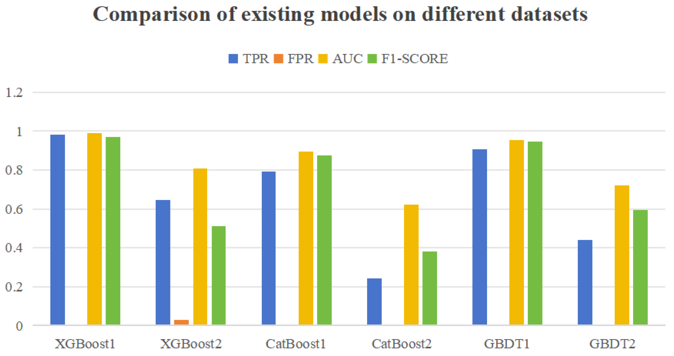
As mentioned earlier, existing hard disk failure prediction methods are applicable on high-quality datasets but have poor performance on low-quality datasets. By using XGBoost, CatBoost, and GBDT models, experiments were conducted on high-quality datasets without data loss and low-quality datasets with 80% loss, as shown in Figure 3. The results were XGBoost1, CatBoost1, and GBDT1 on high-quality datasets, and XGBoost2, CatBoost2, and GBDT2 on low-quality datasets.
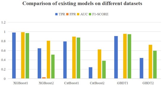
Figure 3.
Comparison of existing models on different datasets.
From the figure, it can be seen that the predictive performance of the three models on low-quality datasets has decreased to varying degrees compared to high-quality datasets, indicating that the existing models are not suitable for low-quality datasets.
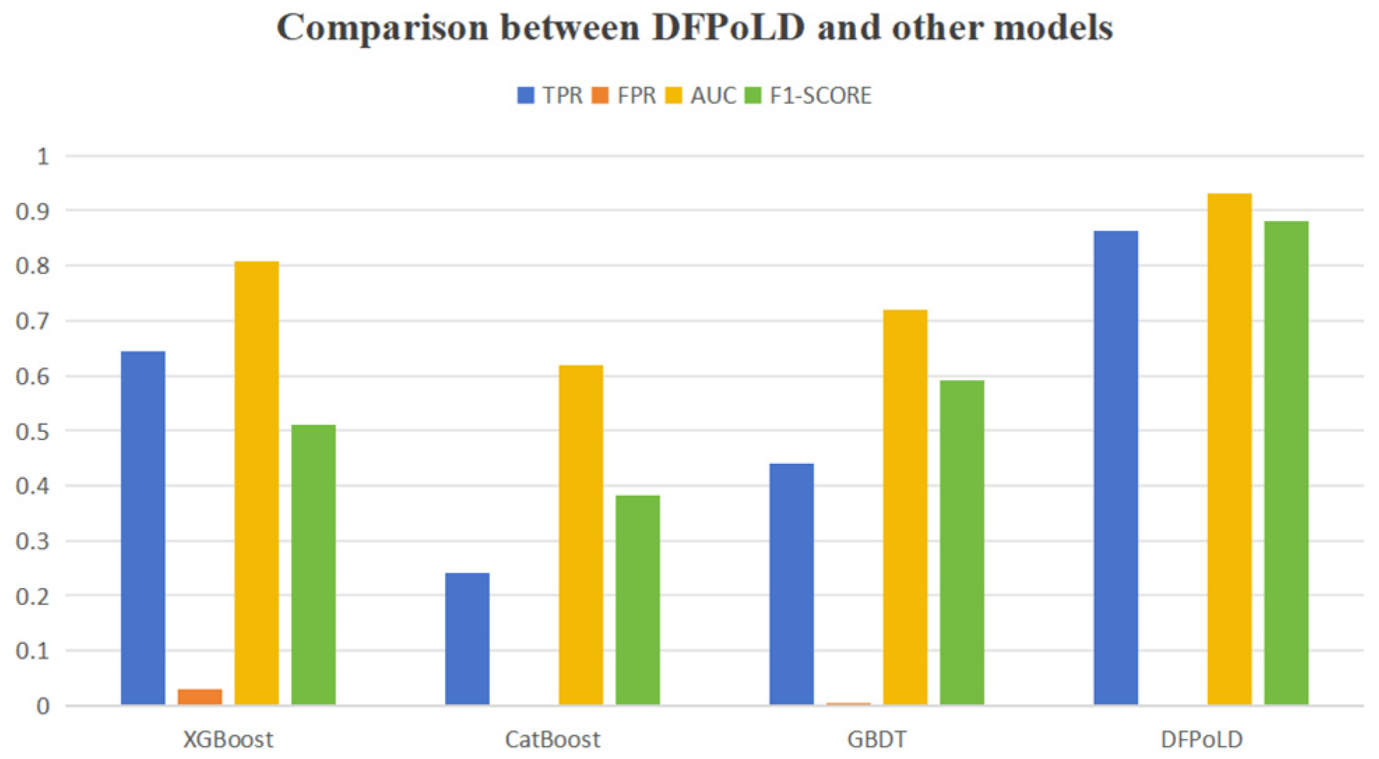
To demonstrate the advantages of DFPoLD over existing models, we compared XGBoost, CatBoost, and GBDT with our proposed model DFPoLD on a low-quality dataset with 80% data loss. The result is shown in Figure 4.
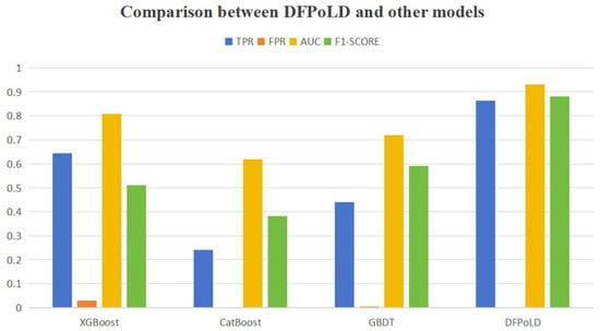
Figure 4.
Comparison between DFPoLD and other models.
From the figure, it can be seen that our proposed model DFPoLD achieves high values in TPR, AUC, and F1 score, significantly better than the other three models, and has a lower FPR. This proves the advantages of our model on low-quality datasets.
6.5. Model Comparison and Selection
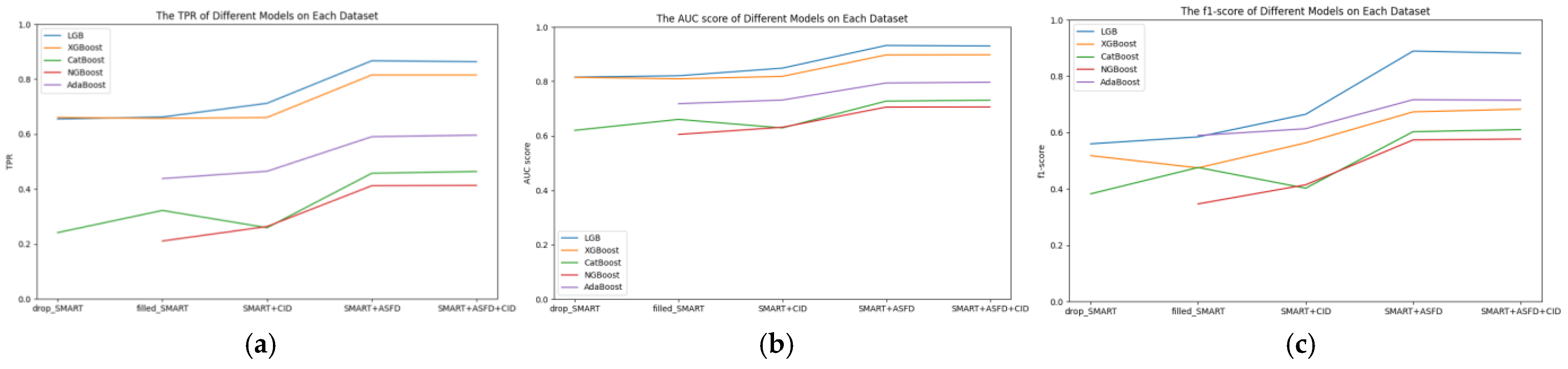
To observe the variation in the effectiveness of hard disk failure prediction across different models, this experiment contrasts the training results on the drop_SMART dataset with 80% of the data removed, the filled_SMART dataset with missing values filled column-wise, the SMART+CID dataset, the SMART+ASFD dataset, and the SMART+ASFD+CID dataset. Various models, including LGB, XGBoost, CatBoost, NGBoost, and AdaBoost, were employed for training. It is important to note that the NGBoost and AdaBoost models require datasets without missing values, hence the absence of results for the drop_SMART dataset in the NGBoost and AdaBoost training in the figures.
Figure 5 illustrates the performance of different models across various datasets. The horizontal axis represents five different datasets, while the vertical axis indicates the scores of different metrics for each model under the respective dataset. In Figure 5a, we observe the effect of different models on TPR. In Figure 5b, the impact of different models on the AUC score is depicted, and in Figure 5c, the influence of different models on the F1 score is shown. From the graph, we can discern that:
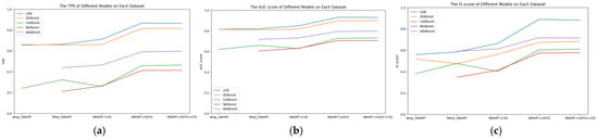
Figure 5.
(a) TPR of different models on each dataset. (b) AUC score of different models on each dataset. (c) F1 score of different models on each dataset.
- (1)
- The effectiveness of the five models varies across different metrics in hard drive failure prediction, with the overall results showing that the LGB model performs the best in terms of TPR, AUC score, and F1 score.
- (2)
- Both the LGB and XGBoost models demonstrate good performance in the TPR and AUC score metrics for hard drive failure prediction. In comparison, the CatBoost and NGBoost models exhibit less favorable results.
- (3)
- While AdaBoost performs poorly in the TPR and AUC score metrics, it achieves relatively high scores in the F1 score metric.
- (4)
- After deleting 80% of the data, the XGBoost model achieves the highest TPR score, reaching 0.6605. However, when the dataset with deleted entries is filled with mode values, the LGB model surpasses XGBoost in TPR. With the addition of time series indicators, the LGB model still performs the best, with the highest TPR reaching 0.8669.
- (5)
- The addition of CID to the filled dataset has a detrimental effect on the CatBoost model, while it has a positive correlation with other models.
- (6)
- Adding ASFD to the filled dataset results in a significant improvement in TPR for all models, indicating the effectiveness of ASFD time series indicators in hard drive failure prediction.
- (7)
- When ASFD and CID are both applied to the dataset, the TPR is almost identical to when ASFD is used alone, suggesting that ASFD is more suitable for hard drive failure prediction scenarios.
To observe how dataset quality impacts failure prediction performance across different models, this experiment compares the training results of LGB, XGBoost, and CatBoost on the drop_SMART dataset, which was constructed by removing 10% to 99% of the data. Models such as NGBoost and AdaBoost were excluded from the experiment due to their requirement for datasets to be free of missing values.
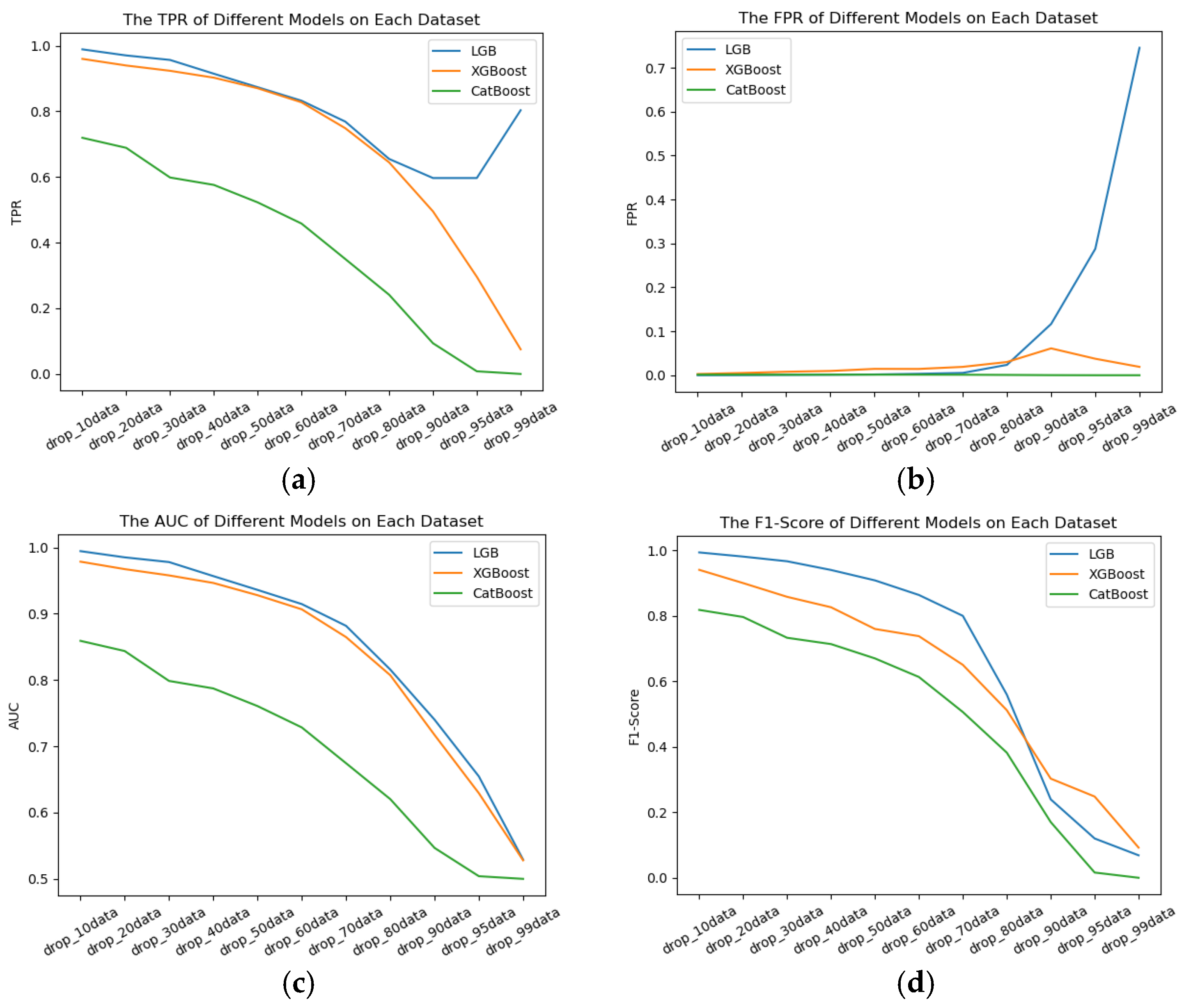
Figure 6 illustrates the performance of different models on different datasets of different qualities. The horizontal axis represents 11 datasets of different qualities, and the vertical axis indicates the scores of different metrics for each model under the respective dataset. In Figure 6a, we observe the effect of different models on TPR, and Figure 6b represents the FPR performance of different models. In Figure 6c, the impact of different models on the AUC score is depicted, and in Figure 6d, the influence of different models on the F1 score is shown. From the graph, we can discern that:
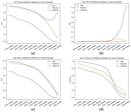
Figure 6.
(a) The effect of TPR for different models on different dataset qualities. (b) The effect of FPR for different models on different dataset qualities. (c) The effect of AUC score for different models on different dataset qualities. (d) The effect of F1 score for different models on different dataset qualities.
- (1)
- Across datasets of varying quality, the three models exhibit different performance levels for hard disk failure prediction. The LGB model consistently achieves the best overall results in terms of TPR and AUC score.
- (2)
- For XGBoost and CatBoost, as dataset quality deteriorates, their TPR, AUC score, and F1 score metrics exhibit a clear downward trend.
- (3)
- When data loss exceeds 95%, TPR begins to recover; however, FPR simultaneously increases, indicating that the LGB model misclassifies a large number of hard disks as faulty, resulting in no overall improvement in performance.
- (4)
- Although CatBoost performs poorly in terms of TPR, AUC score, and F1 score, it achieves excellent and stable results for FPR, remaining close to 0. This suggests that the declining dataset quality does not impact FPR when using the CatBoost model.
- (5)
- When data loss exceeds 70%, the FPR of the LGB model rises sharply, suggesting that higher data loss leads to an increased false positive rate in hard disk failure predictions.
- (6)
- LGB and XGBoost deliver comparable and strong performance on the AUC metric, whereas the CatBoost model shows relatively inferior results.
- (7)
- For datasets with less than 70% data loss, the LGB model outperforms XGBoost and CatBoost across all metrics, making it the preferred choice.
- (8)
- A comprehensive analysis of the four metrics indicates that dataset quality has a significant impact on hard disk failure prediction performance. High-quality datasets yield superior results, while low-quality datasets lead to poorer performance.
To observe the changes in predicting the probability of hard disk failure over time in different models. We set the time window to 30 days. Comparisons were made between models trained on the SMART dataset with 99% data loss, including LGB, CatBoost, and XGBoost, and models trained on the SMART+ASFD dataset with 99% data loss, namely LGB (LGB2), CatBoost (CatBoost2), and XGBoost (XGBoost2).
The horizontal axis represents the number of days before failure. When the horizontal axis is n, it indicates n days remain before the hard disk failure occurs (the axis progresses forward in time; larger values indicate a longer time until failure). The vertical axis represents the average probability that a failing hard disk in the test set is predicted to fail on day x prior to the actual failure. From Figure 7, the following observations can be made:
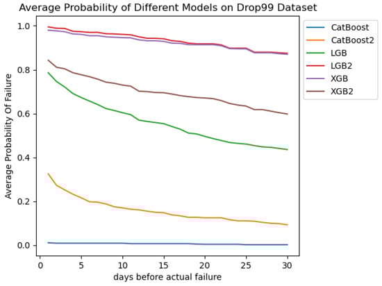
Figure 7.
Change in probability of failure disk being predicted as failure with time.
- (1)
- Before incorporating time-series features, the XGB model outperforms other algorithms. However, after adding time-series features, the predicted failure probabilities decrease. Conversely, the LGB model surpasses the XGB model without the addition of features after integrating the ASFD feature.
- (2)
- After adding the ASFD feature to the dataset, the LGB and CatBoost models significantly outperform their pre-integration counterparts, with a marked improvement in predicting failure probabilities for failing hard disks. This indicates that the ASFD time-series feature introduced in this study is effective for hard disk failure prediction, particularly in scenarios with substantial data loss.
- (3)
- For the LGB model, before incorporating the ASFD time-series feature, the probability of predicting hard disks as likely to fail decreases steadily as the time increases. After integrating the feature, the failure prediction probabilities stabilize over time and remain high even 30 days prior to failure. This demonstrates that the ASFD time-series feature enhances the predictive accuracy by encoding historical hard disk information into each day’s data, improving the likelihood of accurately predicting failures and allowing earlier detection of hard disk failures.
6.6. Experiment on Time Window Selection
To observe the temporal variation in the probability of a hard disk being predicted as faulty across different models on datasets of varying quality, and to determine the optimal time window, we set the time window to 30 days. Comparisons were made using LGB, CatBoost, XGBoost, GBDT, and LR on SMART datasets with 10%, 50%, and 99% data loss.
Figure 8 illustrates the variation in the probability of hard disks being predicted as faulty across different models on datasets of varying quality over time. The meanings of the horizontal and vertical axes are identical to those in Figure 7. Figure 8a–c depict the average probability of failure prediction for faulty hard disks using LGB, CatBoost, XGBoost, GBDT, and LR on datasets with 10%, 50%, and 99% data loss. The following observations can be made:
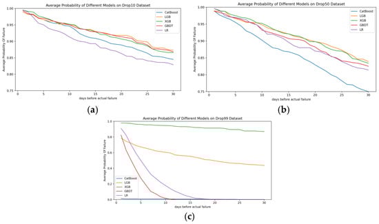
Figure 8.
(a) The probability of different models predicting the failure of hard disks on a dataset with 10% data loss. (b) The probability of different models predicting the failure of hard disks on a dataset with 50% data loss. (c) The probability of different models predicting the failure of hard disks on a dataset with 99% data loss.
- (1)
- As dataset quality decreases, the probability of predicting failure for hard disks decreases more sharply as the time to failure increases. This indicates that lower dataset quality reduces the likelihood of predicting failures in advance, delaying the prediction of hard disk failures.
- (2)
- For datasets with 10% data loss, GBDT demonstrates superior predictive performance. However, as dataset quality declines, the performance of GBDT becomes weaker compared to other models.
- (3)
- Under the extreme condition of 99% data loss, CatBoost is almost incapable of predicting hard disk failures. GBDT and LR can predict failures within 10 and 15 days before failure, respectively, and both show a relatively high probability of predicting failures three days in advance.
- (4)
- Regardless of dataset quality, the LGB and XGB models consistently exhibit strong predictive performance. Their prediction probabilities stabilize over time, indicating that these models perform better than others in predicting failures well in advance.
- (5)
- From Figure 8a–c, it is evident that the probability of predicting failures experiences turning points around 16, 21, and 26 days, respectively, after which the decrease in probability tends to flatten out. This suggests that dataset quality influences the selection of time windows. The worse the quality of the dataset, the longer the selection of time windows should be.
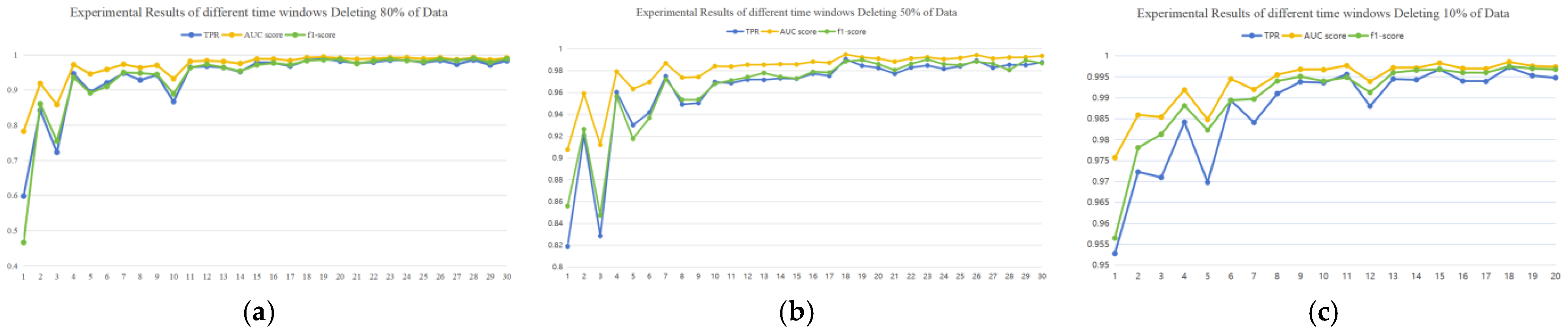
To observe the impact of different time window settings on the performance of the LGB model across datasets of varying quality, we set time windows ranging from 1 to 30 days. Datasets were constructed by removing 10%, 50%, and 80% of the data, processed using the previously described method for handling low-quality datasets, and augmented with the ASFD time-series feature. The LGB model was then trained on these datasets. The experimental results are presented in the following table.
Table 8, Table 9 and Table 10 and Figure 9 present the training results of the LGB model on datasets with 80%, 50%, and 10% data loss, respectively, after incorporating the ASFD feature. From Table 10, it is evident that for the dataset with 10% data loss, the performance of all four metrics stabilizes when the time window is set to 13 days or longer. Therefore, we did not test time windows beyond 20 days. Figure 9 visually illustrates the trend of data change of Table 8, Table 9 and Table 10 in the form of graphs. The key observations from the tables and figure are as follows:
Table 8.
Experimental results of different time windows deleting 80% of data.
Table 9.
Experimental results of different time windows deleting 50% of data.
Table 10.
Experimental results of different time windows deleting 10% of data.
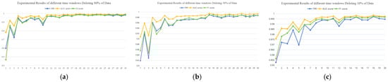
Figure 9.
(a) Experimental results of different time windows deleting 80% of data. (b) Experimental results of different time windows deleting 50% of data. (c) Experimental results of different time windows deleting 10% of data.
- (1)
- For datasets with 80% data loss, a time window of 28 days achieves the best overall performance, with a TPR of 0.9852, an AUC score of 0.9925, and an F1 score of 0.9902, all while maintaining an FPR below 0.02%.
- (2)
- For datasets with 50% data loss, a time window of 23 days provides optimal results, achieving a TPR of 0.9849, an AUC score of 0.9924, and an F1 score of 0.9905, with an FPR below 0.015%.
- (3)
- For datasets with 10% data loss, a time window of 18 days results in the best performance, with a TPR of 0.9973, an AUC score of 0.9986, and an F1 score of 0.9975, while keeping the FPR below 0.01%.
- (4)
- Through the above experiment, we can conclude that when 10%, 50%, and 80% of data are lost, 18, 23, and 28 days are selected as the optimal time windows, respectively. Fit the above data to obtain the time window selection formula in Section 3. Furthermore, we observe that as dataset quality decreases, the optimal time window lengthens, further supporting the correctness of our hypothesis.
6.7. Experiment on Effectiveness of Model and Predicting Failure Days in Advance
To validate the effectiveness of our hard disk failure prediction model, we conducted experiments on a dataset collected from the Nankai-Baidu Joint Lab at Nankai University [32]. The dataset was processed using the methods described earlier. The processed low-quality datasets have been open sourced (https://github.com/cccat-best/Backblaze-.git (accessed on 17 January 2025)). This includes four parts: NanKai-0, NanKai-10, NanKai-50, and NanKai-80, which, respectively, represent the addition of ASFD time series features in datasets that do not lose data, and lose 10%, 50%, and 80% of data. The datasets are available at Open Science Framework (https://osf.io/6xd2a (accessed on 17 January 2025)) with a DOI of https://doi.org/10.17605/OSF.IO/6XD2A, and allocate license CC0 1.0 Universal. The experimental results are as follows.
From Table 11, it can be observed that after incorporating the ASFD feature, datasets of varying quality achieve results on TPR, FPR, AUC score, and F1 score that are nearly equivalent to those of the dataset without data loss. This indicates that ASFD, by reflecting the absolute fluctuations between adjacent SMART data observations, amplifies the differences between positive and negative samples, thereby significantly enhancing hard disk failure prediction. Even in low-quality dataset scenarios, the prediction results are very close to those obtained from the original dataset. This proves that our hard disk failure prediction model for low-quality datasets can accurately predict hard disk failures even if hard disk data is lost, and the prediction performance is close to that of hard disk failure prediction without lost data. This enables us to accurately predict hard disk failures even in practical industrial applications where some data is lost due to objective or subjective reasons during the collection, transmission, storage, and other processes of hard disk data. The loss of data no longer affects the prediction performance.
Table 11.
Test set prediction results of Naikai datasets.
The above results demonstrate that our hard disk failure prediction model for low-quality datasets achieves ideal performance even on real-world datasets. This validates the effectiveness and generalizability of our model.
As mentioned earlier, before training the model, we reset the labels of the ST4000DM000 model hard disk dataset publicly released by Backblaze in 2022. In order to facilitate the calculation of DPF, we uniformly set the time window to 10 days, which ensures that failure hard disks can be detected before they fail. In this experiment, we used the LGB model and extracted all the time data of the failing hard disks of the ST4000DM000 model publicly released by Backblaze in 2023 as the test set. The ideal result would be that all data are predicted as 1. The actual results are shown in Table 12. There are 560 failing disks in the test set, with a total data volume of 87,995.
Table 12.
Test set prediction results.
Table 12 presents the predictions made by the trained model on the test set. It can be observed that the DPF (Days to Predict Failure) obtained from different proportions of data deletion are all above 9.5 days, with a variance of less than 0.06, indicating stable results. In other words, we can predict that the suspected disk will take on average above 9.5 days before it will fail. Therefore, we can conclude that the proportion of data deletion has little to no effect on DPF. Our model can still predict failing disks with a lead time of up to 9.75 days, even when 80% of the data is deleted. This has significant implications for ensuring data reliability in industrial applications.
7. Conclusions
In response to the issue of poor-quality datasets collected in industrial settings, this paper proposes DFPoLD, a time-series feature-based hard disk failure prediction method tailored for low-quality datasets. Using the publicly available 2022 dataset from Backblaze for the ST4000DM000 model, we systematically deleted 10% to 99% of the data to create the low-quality dataset Backblaze-. Through experiments on LGB models with different quality datasets, it is concluded that the higher the dataset quality, the higher the upper limit of the accuracy of hard disk failure prediction, and vice versa. After constructing a low-quality dataset, we introduced ASFD and CID as time-series features to the dataset. The experimental results demonstrate that both ASFD and CID significantly enhance hard drive failure prediction, with ASFD being particularly well-suited for this application. Regarding the issue of time window selection, research was conducted on different models and datasets of varying quality by setting the time window to 30 days. The experimental results indicate that the poorer the quality of the dataset, the longer the time window selection should be, and a time window selection formula is proposed. The hard disk failure prediction model DFPoLD proposed in this article can achieve a True Positive Rate (TPR) of 99.46%, with an AUC score of 0.9971 and an F1 score of 0.9871, while ensuring a False Positive Rate (FPR) of less than 0.04% in the absence of 80% data loss in the dataset.
There are still some limitations in this work. In our exploration of time-series features, we only utilized ASFD and CID. In future research, we will explore more time-series features to enhance hard disk failure prediction, and explore whether it can maintain good hard disk failure prediction performance even after 99% data deletion. In addition, this article selects the SMART data of the ST4000DM000 model hard drive from the S hard drive provider as the initial dataset. Only HDD hard drives, were considered. In the future, we will continue to explore fault prediction methods on SSDs and verify the generality of our method on SSDs.
Author Contributions
Conceptualization, S.W. and H.Y.; data curation, S.W. and X.L.; formal analysis, C.T.; funding acquisition, J.G.; investigation, X.L.; methodology, S.W. and X.L.; project administration, Y.F. and H.Y.; resources, H.S.; software, S.W. and X.L.; supervision, H.Y.; validation, visualization, X.L.; roles/writing—original draft, S.W. and X.L.; and writing—review and editing, Y.F. and H.Y. All authors have read and agreed to the published version of the manuscript.
Funding
This research was supported by a grant from the Tianjin Manufacturing High Quality Development Special Foundation (20232185), the National Key R&D Program of China (2021YFB3300903), the National Natural Science Foundation of China (U23A20299), the Kingbase Foundation (2024-CN-FW-0287), and the Roycom Foundation (70306901).
Institutional Review Board Statement
Not applicable.
Informed Consent Statement
Not applicable.
Data Availability Statement
The original data presented in the study are openly available in OSF at https://osf.io/6xd2a (accessed on 17 January 2025).
Acknowledgments
The authors would like to thank all the anonymous reviewers for their helpful comments and suggestions. We also thank Wenrui Zhang, Jiahua Tong, and Ping Wang for their test work and helpful discussion.
Conflicts of Interest
Author Jiangpu Guo was employed by the company Roycom Information Technology Corporation. The remaining authors declare that the research was conducted in the absence of any commercial or financial relationships that could be construed as a potential conflict of interest.
Abbreviations
| ASFD | Absolute Sum of First Difference |
| TPR | True Positive Rate |
| FPR | False Positive Rate |
| CID | Complexity Invariant Distance |
| LGB | LightGBM |
| LSTM | Long Short-Term Memory |
| GANs | Generative Adversarial Networks |
| RGF | Regularized Greedy Forest |
| TCNs | Temporal Convolutional Networks |
| RNNs | Recurrent Neural Networks |
| CNNs | Convolutional Neural Networks |
| SMART | Self-Monitoring Analysis and Reporting Technology |
| RF | Random Forest |
| FDR | Fault Detection Rate |
| FAR | False Alarm Rate |
| MCTR | Mean-Cost-To-Recovery |
| MA | Moving Average |
| DPF | Days to Predict Failure |
References
- Schroeder, B.; Gibson, G.A. Disk failures in the real world: What does an MTTF of 1,000,000 hours mean to you? In Proceedings of the 5th USENIX Conference on File and Storage Technologies, San Jose, CA, USA, 13–16 February 2007; Volume 7, pp. 1–16. [Google Scholar]
- Xu, S.; Xu, X. ConvTrans-TPS: A Convolutional Transformer Model for Disk Failure Prediction in Large-Scale Network Storage Systems. In Proceedings of the 26th International Conference on Computer Supported Cooperative Work in Design (CSCWD), Rio de Janeiro, Brazil, 24–26 May 2023; pp. 1318–1323. [Google Scholar]
- Srinivaas, A.; Sakthivel, N.R.; Nair, B.B. Machine Learning Approaches for Fault Detection in Internal Combustion Engines: A Review and Experimental Investigation. Informatics 2025, 12, 25. [Google Scholar] [CrossRef]
- Zhang, B.; Gao, Y.; Wu, J.; Wang, N.; Wang, Q.; Ren, J. Approach to Predict Software Vulnerability Based on Multiple-Level N-gram Feature Extraction and Heterogeneous Ensemble Learning. Int. J. Softw. Eng. Knowl. Eng. 2022, 32, 1559–1582. [Google Scholar] [CrossRef]
- Shen, J.; Ren, Y.; Wan, J.; Lan, Y.; Yang, X. Hard disk drive failure prediction for mobile edge computing based on an LSTM recurrent neural network. Mob. Inf. Syst. 2021, 2021, 8878364. [Google Scholar] [CrossRef]
- Coursey, A.; Nath, G.; Prabhu, S.; Sengupta, S. Remaining useful life estimation of hard disk drives using bidirectional lstm networks. In Proceedings of the 2021 IEEE International Conference on Big Data, Orlando, Florida, USA, 15–18 December 2021; pp. 4832–4841. [Google Scholar]
- Ahmed, J.; Green, I.I.R.C. Cost aware LSTM model for predicting hard disk drive failures based on extremely imbalanced SMART sensors data. Eng. Appl. Artif. Intell. 2024, 127, 107339. [Google Scholar] [CrossRef]
- Liu, Y.; Guan, Y.; Jiang, T.; Zhou, K.; Wang, H.; Hu, G.; Zhang, J.; Fang, W.; Cheng, Z.; Huang, P. SPAE: Lifelong disk failure prediction via end-to-end GAN-based anomaly detection with ensemble update. Future Gener. Comput. Syst. 2023, 148, 460–471. [Google Scholar] [CrossRef]
- Gargiulo, F.; Duellmann, D.; Arpaia, P.; Moriello, R.S.L. Predicting hard disk failure by means of automatized labeling and machine learning approach. Appl. Sci. 2021, 11, 8293. [Google Scholar] [CrossRef]
- Burrello, A.; Pagliari, D.J.; Bartolini, A.; Benini, L.; Macii, E.; Poncino, M. Predicting hard disk failures in data centers using temporal convolutional neural networks. In Euro-Par 2020: Parallel Processing Workshops, Proceedings of the 26th International Conference on Parallel and Distributed Computing, Warsaw, Poland, 24–28 August, 2020; Springer International Publishing: Berlin/Heidelberg, Germany, 2021; pp. 277–289. [Google Scholar]
- Xu, C.; Wang, G.; Liu, X.; Guo, D.; Liu, T.-Y. Health status assessment and failure prediction for hard drives with recurrent neural networks. IEEE Trans. Comput. 2016, 65, 3502–3508. [Google Scholar] [CrossRef]
- Lu, S.; Luo, B.; Patel, T.; Yao, Y.; Tiwari, D.; Shi, W. Making disk failure predictions SMARTer! In Proceedings of the 18th USENIX Conference on File and Storage Technologies, Boston, MA, USA, 25–27 February 2020; pp. 151–167. [Google Scholar]
- Allen, B. Monitoring hard disks with SMART. Linux J. 2004, 2004, 9. [Google Scholar]
- Jiang, T.; Huang, P.; Zhou, K. Cost-efficiency disk failure prediction via threshold-moving. Concurr. Comput. Pract. Exp. 2020, 32, e5669. [Google Scholar] [CrossRef]
- Zhang, J.; Huang, P.; Zhou, K.; Xie, M.; Schelter, S. HDDse: Enabling High-Dimensional Disk State Embedding for Generic Failure Detection System of Heterogeneous Disks in Large Data Centers. In Proceedings of the 2020 USENIX Annual Technical Conference, Boston, MA, USA, 15–17 July 2020; pp. 111–126. [Google Scholar]
- Wang, H.; Zhuge, Q.; Sha, E.H.-M.; Xu, R.; Song, Y. Optimizing Efficiency of Machine Learning Based Hard Disk Failure Prediction by Two-Layer Classification-Based Feature Selection. Appl. Sci. 2023, 13, 7544. [Google Scholar] [CrossRef]
- Zhang, M.; Ge, W.; Tang, R.; Liu, P. Hard disk failure prediction based on blending ensemble learning. Appl. Sci. 2023, 13, 3288. [Google Scholar] [CrossRef]
- Ge, W.; Liu, P.; Zhang, M.; Zhang, Z.; Lai, Y. DiskTransformer: A Transformer Network for Hard Disk Failure Prediction. In Proceedings of the 7th International Conference on Artificial Intelligence and Big Data (ICAIBD), Beijing, China, 5–7 July 2024; pp. 327–332. [Google Scholar]
- Lu, X.; Tu, C.; Yang, H.; Guo, J.; Sun, H. FPTSF: A Failure Prediction of Hard Disks Based on Time Series Features Towards Low Quality Dataset. In Proceedings of the Asia-Pacific Web (APWeb) and Web-Age Information Management (WAIM) Joint International Conference on Web and Big Data, Jinhua, China, 30 August–1 September 2024; pp. 438–447. [Google Scholar]
- Friedman, J.H. Greedy Function Approximation: A Gradient Boosting Machine. Ann. Stat. 2001, 29, 1189–1232. [Google Scholar] [CrossRef]
- Han, S.; Wu, J.; Xu, E.; He, C. Robust Data Preprocessing for Machine-Learning-Based Disk Failure Prediction in Cloud Production Environments. arXiv 2019, arXiv:1912.09722. [Google Scholar]
- Wang, H.; Yang, Y.; Yang, H. Hard Disk Failure Prediction Based on Lightgbm with CID. In Proceedings of the 2021 IEEE Symposium on Computers and Communications (ISCC), Athens, Greece, 5–8 September 2021; pp. 1–7. [Google Scholar]
- Ke, G.; Meng, Q.; Finley, T.; Wang, T.; Chen, W.; Ma, W.; Ye, Q.; Liu, T.-Y. Lightgbm: A highly efficient gradient boosting decision tree. In Proceedings of the 31st Conference on Neural Information Processing Systems (NIPS 2017), Long Beach, CA, USA, 4–9 December 2017; pp. 3149–3157. Available online: https://dl.acm.org/doi/10.5555/3294996.3295074 (accessed on 4 December 2017).
- Priyadarshini, I.; Cotton, C. A novel LSTM–CNN–grid search-based deep neural network for sentiment analysis. J. Supercomput. 2021, 77, 13911–13932. [Google Scholar] [CrossRef] [PubMed]
- Belete, D.M.; Huchaiah, M.D. Grid search in hyperparameter optimization of machine learning models for prediction of HIV/AIDS test results. Int. J. Comput. Appl. 2022, 44, 875–886. [Google Scholar] [CrossRef]
- Sun, Y.; Ding, S.; Zhang, Z.; Jia, W. An improved grid search algorithm to optimize SVR for prediction. Soft Comput. 2021, 25, 5633–5644. [Google Scholar] [CrossRef]
- Shekhar, S.; Bansode, A.; Salim, A. A comparative study of hyper-parameter optimization tools. In Proceedings of the 2021 IEEE Asia-Pacific Conference on Computer Science and Data Engineering (CSDE), Brisbane, Australia, 8–10 December 2021; pp. 1–6. [Google Scholar]
- Yang, L.; Shami, A. On hyperparameter optimization of machine learning algorithms: Theory and practice. Neurocomputing 2020, 415, 295–316. [Google Scholar] [CrossRef]
- Zhang, J.; Wang, Q.; Shen, W. Hyper-parameter optimization of multiple machine learning algorithms for molecular property prediction using hyperopt library. Chin. J. Chem. Eng. 2022, 52, 115–125. [Google Scholar] [CrossRef]
- Akiba, T.; Sano, S.; Yanase, T.; Ohta, T.; Koyama, M. Optuna: A next-generation hyperparameter optimization framework. In Proceedings of the 25th ACM SIGKDD International Conference on Knowledge Discovery & Data Mining. Anchorage, AK, USA, 4–8 August 2019; pp. 2623–2631. [Google Scholar]
- Lai, J.P.; Lin, Y.L.; Lin, H.C.; Shih, C.Y.; Wang, Y.P.; Pai, P.F. Tree-based machine learning models with optuna in predicting impedance values for circuit analysis. Micromachines 2023, 14, 265. [Google Scholar] [CrossRef] [PubMed]
- Li, J.; Stones, R.J.; Wang, G.; Liu, X.; Li, Z.; Xu, M. Hard drive failure prediction using decision trees. Reliab. Eng. Syst. Saf. 2017, 164, 55–65. [Google Scholar] [CrossRef]


Disclaimer/Publisher’s Note: The statements, opinions and data contained in all publications are solely those of the individual author(s) and contributor(s) and not of MDPI and/or the editor(s). MDPI and/or the editor(s) disclaim responsibility for any injury to people or property resulting from any ideas, methods, instructions or products referred to in the content. |
© 2025 by the authors. Licensee MDPI, Basel, Switzerland. This article is an open access article distributed under the terms and conditions of the Creative Commons Attribution (CC BY) license (https://creativecommons.org/licenses/by/4.0/).