Abstract
For the last decade, social networking services (SNS), such as X, Facebook, and Instagram, have become mainstream media for advertising and marketing. In SNS marketing, word-of-mouth among users can spread posted advertising information, which is known as viral marketing. In this study, we first analyzed the time series of user reactions to Instagram posts to clarify the characteristics of user behavior. Second, we modeled these variations using statistical distributions to predict the information diffusion of future posts and to provide some insights into the factors that affect users’ reactions on Instagram using the estimated parameters of the modeling. Our results demonstrate that user reactions have a peak value immediately after posting and decrease drastically and exponentially as time elapses. In addition, modeling with the Weibull distribution is the most suitable for user reactions, and the estimated parameters help identify key factors that influence user reactions.
1. Introduction
Until the Internet became as widespread as it is today, television, radio, magazines, and newspapers were the mainstream media for advertising. Above all, television has had a particularly significant influence on many people, and being featured on it has greatly contributed to the spread of information. However, with the rapid spread of the Internet, the devices used to access information have also shifted significantly from personal computers to smartphones and tablets [1]. This technological evolution has, in turn, instigated a major transition in advertising and marketing systems. Social networking services (SNS), such as X (formerly Twitter) and Facebook, have emerged as a primary means of information diffusion on the Internet, allowing people to easily connect with strangers online who share similar interests and tastes, in addition to maintaining face-to-face friendships. In Japan, a statistical report [2] indicates that, for the first time, Internet advertising expenditures surpassed that of television in 2021, establishing SNS as a central and significant platform for advertising [3].
On SNS, users often acquire information by following accounts that post information about things that they are interested in or want to know about. When using an SNS as a means of advertising, it is important to make users aware of their accounts and how to have them follow their accounts. Companies can immediately and directly advertise to users following their accounts on SNS postings, and the cost is lower than that of the conventional mass media [4]. Authors in [5] revealed that many influencers, who have a larger number of followers, post about several brands (company names, etc.), and their posting patterns change depending on the influencer’s popularity. For example, reviews of products that influencers have experienced tend to have a large number of characters and few hashtags, and when posting a brand name, there is only one hashtag, based on large-scale data. Authors in [6] investigated the influence of influencers using a non-network approach and suggested that posts by influencers with a relatively small number of followers influence users more effectively. Moreover, Ref. [7] proposed a method using machine learning to find posts that were actually requested from sponsors (Sponsored posts) from post data that appear to be unsponsored (Non-sponsored posts). In addition to influencer-based campaigns, the timing, frequency, and content of posts from any account significantly influence user responses. For example, previous studies have explored predictive modeling using hashtags and content features [8], developed multi-platform recommendation systems [9], and investigated cost-effective advertising strategies [10]. Business intelligence techniques have also been employed to support marketing decisions across different SNS platforms, providing valuable insights for strategic planning [11].
Numerous studies have examined social media advertising; however, the dynamics of user engagement over time for posts from corporate accounts have not been sufficiently investigated. Corporate content stands distinct from influencer content because it is explicitly branded and promotional. This inherent characteristic may lead to different user behaviors compared to influencer content. When influencers post on SNS, people often feel more connected and engaged. This is because influencers are perceived as authentic, and they build a kind of one-sided friendship with their followers. In contrast, when companies post, users tend to be more selective in their engagement, or even somewhat skeptical [12]. These differences have been shown not only to change how many people engage; they also affect how long that engagement lasts [13]. Even though many people know this from experience, few studies have provided a direct statistical comparison of engagement decay patterns across both types of accounts. These studies further emphasize the importance of investigating information diffusion processes and branding strategies specific to corporate social media accounts. This is one of the important objectives that our paper aims to address. Furthermore, such corporate advertising posts often follow internal marketing strategies that are not publicly disclosed, making it challenging for outsiders to infer their effectiveness and optimize their impact. Understanding how users interact with corporate posts over time is a key consideration for enhancing marketing effectiveness. Previous studies have proposed various mathematical models to capture such engagement decay, including well-known functional forms like the exponential, power-law, logistic, and Bass models [14,15]. Among these, the Weibull distribution has garnered attention due to its remarkable flexibility in modeling both rapid initial drops in engagement and the longer-tailed nature observed in digital content diffusion [16,17].
SNS platforms are evolving through trial and error to maximize user engagement, such as “likes” and comments, which have become important factors in advertising effectiveness. However, most previous studies have focused on influencer marketing or general content diffusion, while user reactions to posts from official business accounts have not been sufficiently considered. Unlike influencer posts, in which the line between personal and promotional content tends to be ambiguous, posts from verified business accounts are perceived as SNS advertisements and may trigger different user engagement patterns. We consider it necessary to investigate how this difference affects the dynamics of user behavior surrounding business social media activity.
Based on the background described above, we analyze a long-term user engagement with Instagram posts from official business accounts. Specifically, we investigate how users react to advertising posts over time by periodically collecting timeline data using the Instagram Graph API [18]. In this paper, we define user engagement in terms of the number of “likes” received by each post and focus on the time-series variation of this factor to clarify the characteristics of user reactions. To quantitatively capture this variation, we modeled the time series of “likes” using four well-known functional forms: Logistic, Exponential, Weibull, and Log-normal distributions. To evaluate modeling accuracy, we used two standard statistical measures: Root Mean Square Error (RMSE), which assesses the average deviation from the observed data, and the Akaike Information Criterion (AIC), which accounts for both the fit and model complexity. Our empirical results demonstrate that the Weibull distribution consistently outperforms the other models across both evaluation metrics. These findings provide the utility of Weibull-based modeling for understanding and predicting engagement trends in corporate social media advertising and offer practical insights for optimizing posting strategies and evaluating campaign effectiveness.
2. Materials and Methods
2.1. Measurement Methodology
Here, we describe 8 Instagram business accounts from which we obtain timelines and details of measurement procedures using the Instagram Graph API.
2.1.1. Target Business Accounts
We focused on 8 Instagram business accounts (Account A to H) in order to satisfy the following criteria.
- Highly frequent posting (multiple posts per week)
- Same posts as other social networking services (X, etc.)
- Different genres compared to other accounts
Table 1 shows the detailed descriptions of the selected accounts. In the table, the “Account Label” column shows a confidential label for each selected business account. “Headquarters” indicates the head office location for each account, and “# of followers” represents the number of followers at the time of measurement. Detailed information about each business account is provided under the “Description” column.
Although concerns regarding the geographic bias and representativeness of the selected business accounts exist, we have endeavored to mitigate these concerns by considering a diverse range of geographical locations, follower counts, and genres during the selection process. We believe that the proposed approach enabled us to extract significant patterns from the current dataset. Nonetheless, a more thorough examination would require a significantly larger and more varied collection of data. However, due to the rate limitations of the Instagram Graph API, access to such extensive data was restricted in this study. We recognize the necessity of leveraging large-scale datasets to further demonstrate the utility and generalizability of the findings presented in this paper. In addition, this study did not differentiate between image and video content in the analysis. As engagement dynamics can vary significantly between static and motion media, future research should address this limitation by categorizing and analyzing posts according to content type.
2.1.2. Obtaining Timeline Data
First, we created a standard personal account and then switched it to a business account because the Instagram Graph API can only be accessed through a business account to retrieve timeline data. Subsequently, we registered our application in the business account and obtained the credentials, that are access key and access token, to access the API.

Table 1.
Details of target accounts.
Table 1.
Details of target accounts.
| Account Label | Headquarters | # of Followers (Millions) | Description |
|---|---|---|---|
| A | California, USA | 630 | A major provider of a visual-centric social media service where users primarily share photos and videos. |
| B | Paris, France | 49 | A French luxury fashion brand and one of the world’s most famous luxury brands, that mainly manufactures and sells luxury goods such as leather goods, bags, wallets, accessories, clothing, and shoes. |
| C | Tokyo, Japan | 4.6 | A Japanese cooking site providing daily one-minute cooking recipe videos. It provides cooking enthusiasts and novice cooks with videos of recipes and cooking methods for various cuisines, allowing viewers to easily enjoy cooking at home. |
| D | Oregon, USA | 200 | A United States-based global sporting goods company that company that manufactures and sells sports shoes, apparel, and sporting goods. The company offers several products for sports enthusiasts and athletes woridwide and is particularly well-known for sports such as running, basketball, and soccer. |
| E | California, USA | 4.2 | An online multiplayer strategy game was launched in 2009. After its release, the game became the most popular PC game in the world in 2012. The event has attracted attention as an electronic sports event where professional gamers compete, including the provision of visas to professional athletes in the United States. It has also attracted attention as an electronic sports event where professional gamers compete. |
| F | Tokyo, Japan | 3.2 | A Japanese account managed by one of the world’s largest coffee chains that announces new products and describes how to enjoy these services. |
| G | Manchester, UK | 1 | A UK-based global nutritional supplement brand that primarily sells protein powders and supplements. The company markets several nutritional supplements to fitness enthusiasts, athletes, and the public who are health conscious. |
| H | Florence, Italy | 49 | A global luxury brand based in Italy, offering luxury fashion items, leather goods, accessories, perfumes, and watches. |
Listing 1 shows an example of the Graph API to retrieve the timeline of the target business accounts. In this listing, $USER_ID is the ID number of the previously created business account, and $ACCESS_TOKEN is the authentication token to access the Graph API. The target business accounts are specified in the $account parameter.
| Listing 1. Instagram Graph API. |
| curl -g -X GET “https://graph.facebook.com/v14.0/$USER_ID?fields= business_discovery.username($account){name,followers_count,media {like_count,comments_count,timestamp}}&access_token=$ACCESS_TOKEN” |
This API returns timeline data, that is the latest 20 posts, of the specified account that includes account name, the number of followers, the number of likes, the number of comments, and timestamp. account name is the screen name of the specified account, and the number of followers denotes the number of followers at the time of accessing. like_counts and comments_count are the number of likes and comments on each post on the timeline, respectively. timestamp denotes the posting date and time in GMT for each post.
As mentioned above, the Graph API does not permit retrieval of past posts; thus, we repeatedly accessed the API at 15 min intervals to obtain the time series variations of each timeline as past data. Listing 2 shows an example of a single post of data obtained through the API. The returned data is expressed in JSON format, and id in this Listing is the unique number of posts assigned by Instagram automatically (some numbers have been replaced by asterisks).
| Listing 2. Example of one post data. |
| { “like_count”: 371997, “comments_count”: 43393, “timestamp”: “2022-01-04T17:07:49+0000”, “id”: “17933486782∗∗∗∗∗∗” }, |
As shown in Listing 2, the data returned by accessing the API consists of the post data of the latest 20 posts at the time of accessing. Next, we divide the timeline data into time-series data for each individual post. Listing 3 presents an example of divided post data. The first column shows the access times in the JST time zone. The second column lists the date and time of posting in GMT. The third and fourth columns represent the cumulative numbers of likes and comments, respectively. These divided data show how the number of likes and comments increased immediately after posting. In this Listing, the time of posting is 5 January 2022, 02:07:49 JST; however, the time to access the API was 5 January 2022, 02:15:00 JST. Namely, we obtained this post data after 8 min of posting, and the number of likes increased to 17,552 during the time gap. In our measurement, the time lag between posting and data retrieval was up to 15 min depending on the timing of the post, and the diffusion status during the time gap could not be captured. This issue can be mitigated to some extent by shortening the measurement interval; however, for our analysis, we measured every 15 min, and the analysis will be conducted on the data of postings that were measured with good timing, i.e., captured within 2 min from posting time or the number of likes in the first time slot is below 1000.
| Listing 3. Example of aggregated data. |
| 202201050215 2022-01-04T17:07:49+0000 17552 76 202201050230 2022-01-04T17:07:49+0000 33770 164 202201050245 2022-01-04T17:07:49+0000 43993 222 202201050300 2022-01-04T17:07:49+0000 52310 243 202201050315 2022-01-04T17:07:49+0000 59008 274 202201050330 2022-01-04T17:07:49+0000 65026 293 |
2.1.3. Measurement Period
The measurement period spans from mid-December 2021 to the end of December 2023. A general-purpose PC running Ubuntu Server 22.04 LTS was used. To continuously obtain the timeline data of target accounts, a shell script utilizing the API was executed using cron daemon. In addition, Post data were collected in compliance with the Instagram Graph API’s data use policies.
2.2. Modeling
In this subsection, we model the distribution of the number of likes described in the previous section using probability distributions to gain insights into the factors influencing user responses.
2.2.1. Candidate Distributions
Based on the shapes of the distribution of the number of likes, as described in the previous section, we selected 4 candidate probability distributions for modeling.
Logistic Distribution
The logistic distribution is a continuous probability distribution with an S-shaped curve. Equation (1) shows the probability density function of logistic distribution. The logistic distribution is mainly applied to ecological data analysis, such as modeling individual growth, range expansion, and shifts in species distribution. In economics, it is used for forecasting economic trends, commodity supply and demand, and market growth rates.
where is the location parameter and is the scale parameter.
Exponential Distribution
The exponential distribution is a continuous probability distribution. Equation (2) shows the probability density function of the exponential distribution. It is used to model the event latency and inter-arrival times, such as data packet arrival, transmission interval, communication delays, and network load.
where is the rate parameter and the expected value.
Weibull Distribution
The Weibull distribution is a probability distribution used to quantitatively express the relationship between the size and strength of materials and is mainly used to model failure and degradation rates. Equation (3) shows the probability density function of the Weibull distribution. Based on the results obtained so far, the user response is considered to decay exponentially over time, and the user response can be interpreted as the degradation of the real-time nature of the information in response to the postings.
where m is the shape parameter that determines the shape of the distribution. In addition, is the scale parameter that indicates the variation in density (magnitude and width of peak values).
Log-Normal Distribution
The log-normal distribution is a probability distribution in which the logarithm of the random variable follows a normal distribution. Equation (4) shows the probability density function of the log-normal distribution. This distribution is used in reliability analysis to model the time to failure of electronic components, mechanical parts, and material fatigue. It is particularly effective in modeling failures caused by cumulative effects such as chemical reactions, corrosion, and fatigue crack growth; therefore, we considered it a candidate for modeling the decay in the number of likes.
where , that serves as the location parameter, is the mean of the normal distribution of the natural logarithm of the random variable. , that serves as the scale parameter, is the standard deviation of the normal distribution of the natural logarithm of the random variable.
2.2.2. Parameter Estimation
First, we analyzed the collected “like” count data by calculating the cumulative relative frequency of likes and the elapsed time after posting. Second, these two values, the relative frequency and elapsed time, were then used as inputs to estimate the parameters of various probability distributions. We used the least squares method [19] to estimate the parameters of the 4 probability candidate distributions. The least squares method minimizes the sum of squares errors by taking the difference between each observed value and the corresponding model prediction.
To compare the accuracy of the estimated parameters, two evaluation metrics were used: RMSE and AIC. The RMSE represents the square root of the mean of the squared residuals between the predicted and actual values and is defined as follows.
where is the i-th actual value, and is the i-th predicted value.
The AIC is a widely used statistical metric for model selection. It evaluates how well the prediction model fits the data while penalizing complexity to prevent overfitting. The AIC is calculated as follows.
where k is the number of model parameters, also known as the degrees of freedom, and is the maximized log-likelihood.
We expect that optimal parameter estimation will enable the prediction of the extent and scale of information diffusion in advance. At the same time, it provides a basis for investigating how each model parameter is influenced by user behavior and characteristics both in SNSs and the real world.
3. Results
First, we present the time series variations in users’ reactions to advertising posts and trends at the time of posting on the target business accounts. Next, we describe the results of statistical modeling for the collected data.
3.1. Time Series Variations
In this study, we define the number of likes on each post as user reactions and analyze the time series variation of it.
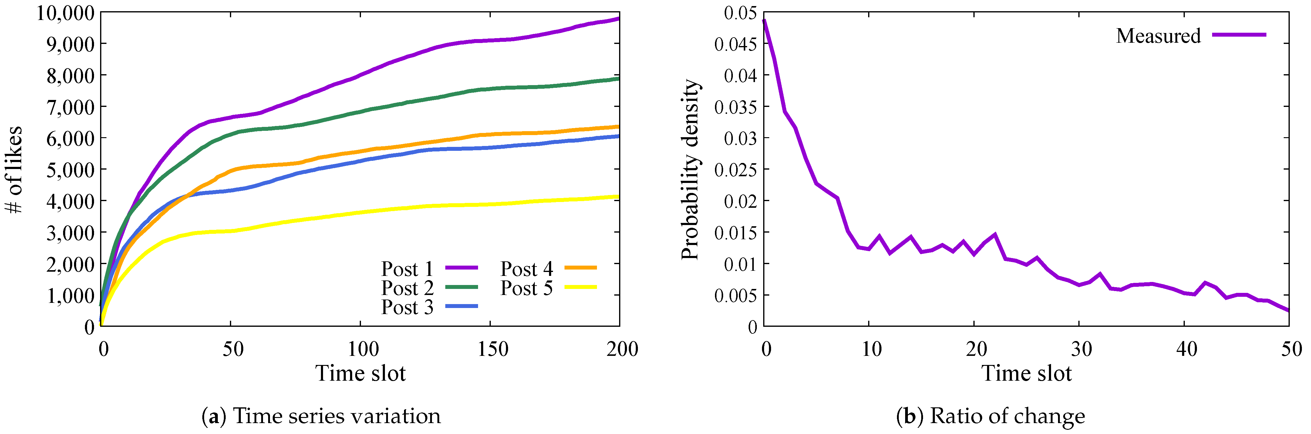
Figure 1 shows variations in the number of likes for posts from Account F. Figure 2 shows the case for Account C. In addition, (a) in each figure denotes the time series variation of likes from the time of posting. The horizontal axis represents the time slot value, which is a time unit of 15 min. A time slot value of 200 corresponds to 20 h after each post. The vertical axis represents the number of likes. Each colored line in these figures denotes a distinct post that was measured shortly after posting. Thus, we show data for five posts measured on each account. (b) of each figure denotes the ratio of change in the number of likes in each time slot. In these figures, the vertical axis represents the ratio of change. We define the ratio of change as the ratio of the increase in each time slot to the total number of likes at time slot 50.
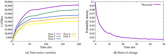
Figure 1.
Variation in # of likes on Account F posts.
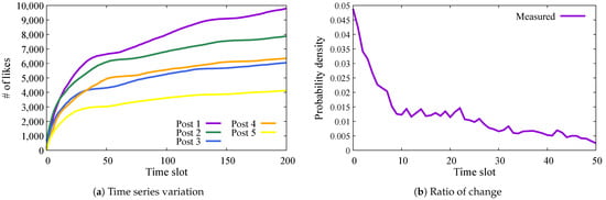
Figure 2.
Variation in # of likes on Account C posts.
As shown in these figures, although there are posts in which users are stably interested in the long term and click the like button, all posts receive the majority of responses immediately after posting, followed by an exponential decline in user engagement. In addition, we infer that the reaction rate at the time of posting determines the degree of user responses, which is the total number of likes. Although we expected that the number of followers would affect the number of likes, the total number of likes observed in Account F is between 20,000 and 50,000, and the ratio to the number of followers, 3.2 million, is between and . Posts on Account C, with 1 million followers, received 4000 to 10,000 likes, corresponding to to of its followers. Although there is a large difference in the actual number of likes, there is no significant difference in these ratios between the two accounts. Moreover, especially in the purple and green lines in Figure 2, the number of likes increases again around time slot 50 after an initial decline. This suggests that users’ responses are influenced by multiple factors, including other SNS platforms and traditional mass media.
Overall, we found that most posts tended to spread rapidly immediately after posting and settled down after a certain time had elapsed. On the other hand, some posts re-spread even after a certain time, which we attribute to the influence of other media.
3.2. Trends in the Time of Posting
Next, we investigate when each account posts on Instagram. Figure 3 show histograms of the time of posting for each account. The horizontal axis represents the time of posting in the GMT time zone, and the vertical axis indicates the number of posts per hour. Due to the posting frequency among accounts, the histograms are split into two figures: Figure 3a denotes the lower posting frequency accounts, and Figure 3b is the higher ones. From Figure 3a, assuming that Account G and Account F are headquartered in Europe and share the GMT time zone, it can be seen that most posts are made during the daytime hours (11:00 to 13:00). Account D and Account E are both headquartered in the United States, and considering the time difference, there are many posts in the morning time. Additionally, from Figure 3b, Account C and Account F are Japanese companies; thus, we found that posts were concentrated in Japanese daytime hours, from 10:00 to 19:00. Since Account B is presumed to be managed in Europe, its posting pattern resembles that of Account G and Account H. Posts from Account A are similarly concentrated at the same times as Account D, suggesting that they were intended to be posted within the United States.
From these observations, we conclude that all business accounts post during daytime hours in local time. This is likely because user activity is lower during nighttime hours, so most posts are made when users are more active during the day.
3.3. Parameter Estimation
As a result of modeling the distributions of the number of likes using candidate distributions, Table 2 shows a summary of the estimated parameter sets. In this table, “# of posts” indicates the number of well-timed posts used for parameter estimation. The estimated parameters shown in this table are the median values computed from individual post-level estimates for each account. For example, of logistic distribution for Account A, which is 62,453.9, is the median of estimated across 30 individual posts.
Table 2.
Estimated parameters.
From Table 2, the number of followers has a significant impact on the magnitude of the engagement metrics. In this comparison, we used the median rather than the mean to summarize parameters, aiming to reduce the impact of outliers and skewed distributions in engagement data. Since some posts receive exceptionally high or low user reactions, the median provides a more robust and representative measure of central tendency for comparing account-level characteristics. For example, Account A with 630 million followers consistently denotes the highest parameter values across all models: Logistic ( = 62,453, s = 104,927.7), Exponential ( = 118,983.5), Weibull ( = 100,356.2), and Log-normal ( = 1.575917, = 54,277.2). In contrast, the estimated parameters of Account F, with fewer followers, have relatively lower scale or dispersion parameters. This relationship indicates that a larger number of followers is a key factor in overall engagement, which is consistent with prior studies in the social media marketing literature. The Weibull shape parameter (m) and the log-normal standard deviation () are relatively consistent values among most accounts, ranging from to for m, from to for . This indicates a long-tailed distribution, in which a small number of posts receive high engagement, while the majority of posts receive modest responses. We consider that such distributional characteristics validate the use of heavy-tailed distributions to represent user behaviors on social media.
Next, to verify the distribution fit, we calculated two statistical measures, RMSE and AIC, based on the parameter estimates, and the results are shown in Table 3. In this table, the statistical measures represent the mean and standard deviation calculated across all posts for each account. From these results, we can see that modeling with the Weibull distribution yields the lowest RMSE and the smallest variance, indicating that it is the optimal distribution among these distributions. A similar conclusion can be drawn from the AIC values. In addition, Figure 4 shows the variation of each statistical measure. The horizontal axis shows each target account, and the vertical axis indicates the RMSE and AIC values. In this figure, data from of all posts are included; the remaining are excluded as outliers. From this figure, although the log-normal distribution has good results in modeling user behaviors, particularly for Account F, the Weibull distribution exhibits comparatively smaller variance overall, and we consider it sufficient to model user behavior with sufficient accuracy for large datasets.
Table 3.
Summary of statistical measures (RMSE and AIC).
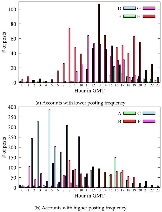
Figure 3.
Characteristics of the time of posting.
Figure 3.
Characteristics of the time of posting.
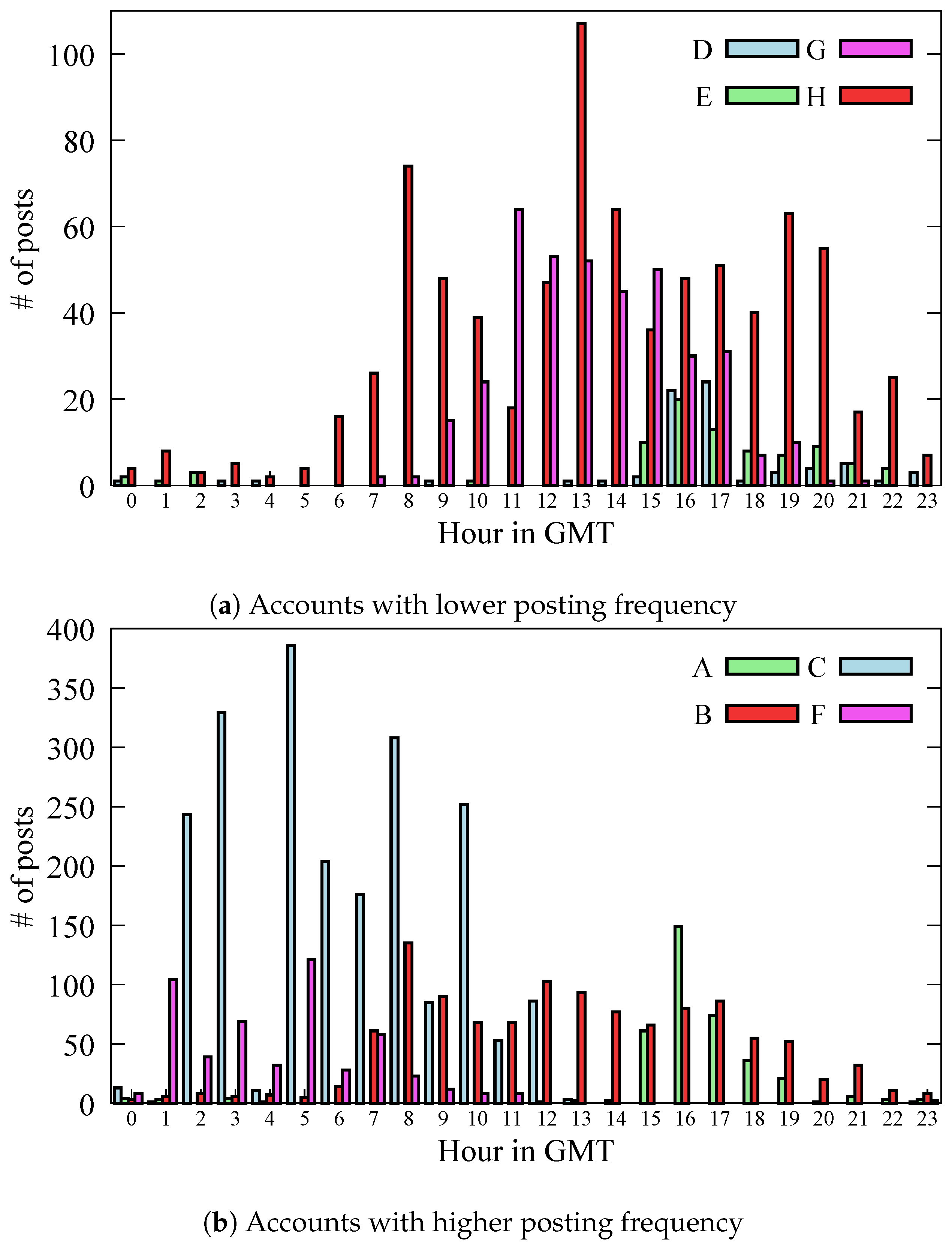
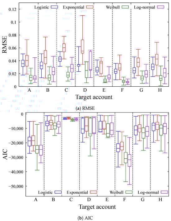
Figure 4.
Boxplot showing quartiles of statistical measures.
Figure 4.
Boxplot showing quartiles of statistical measures.
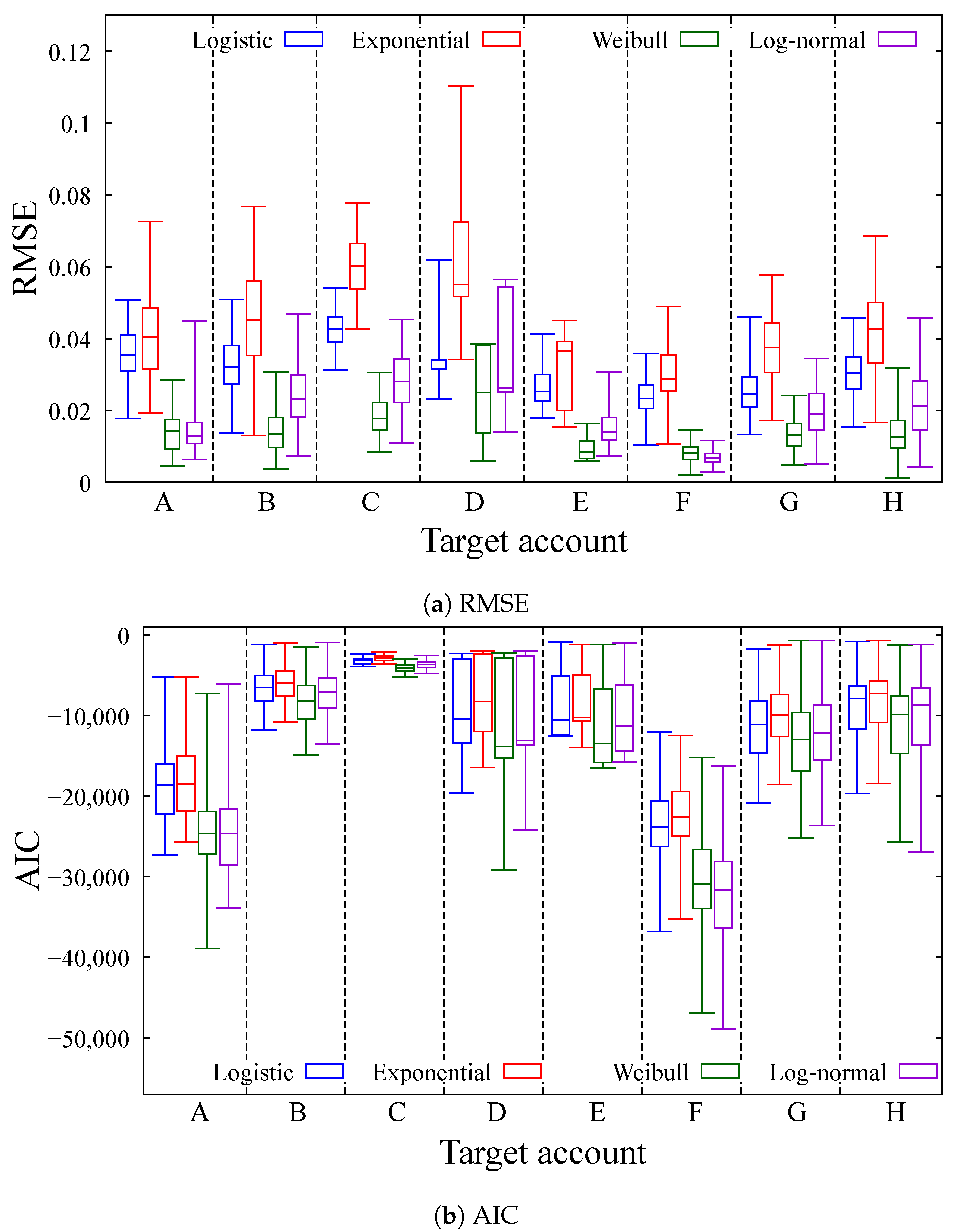
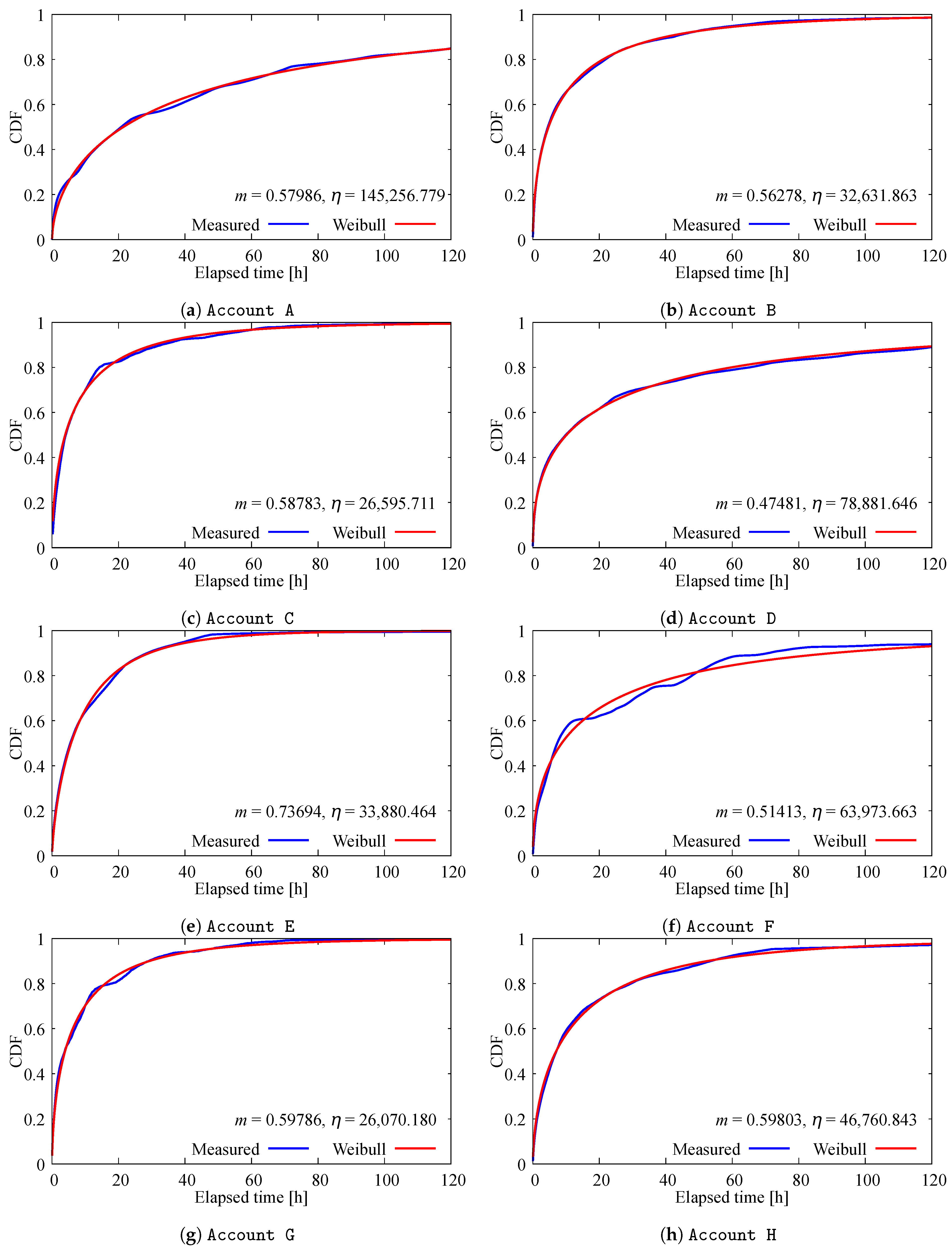
Figure 5 shows the distribution of the number of likes and the probability distribution function of the Weibull distribution using the estimated parameters for each account. In these figures, the horizontal axis represents the elapsed time from the posting time, and the vertical axis represents the cumulative distribution function (CDF). In addition, the estimated parameters of the Weibull distribution are shown at the bottom right of each figure. From these figures, we also consider that our modeling method using the Weibull distribution can accurately express the distribution of the number of likes. These results indicate that user reactions can be considered equivalent to predicting the lifespan (i.e., degradation rate) of a certain product. The fact that user reactions subside as time elapses can be seen as a degradation in the freshness of posts.
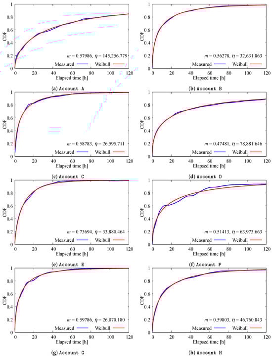
Figure 5.
Graphical comparison with measured data and estimated Weibull distribution.
Next, we discuss the characteristics of the estimated parameters of the Weibull distribution. As noted above, the estimated values of m range from to . In a Weibull distribution, a smaller value of m implies a more heavily skewed distribution with a sharper peak and a longer right tail. This indicates that user reactions are more concentrated immediately after posting, with relatively fewer delayed responses. On the other hand, the values of have a wide range from 28,214 (Account F) to 100,356 (Account A) in our estimation. This parameter determines the position of the peak in the distribution. A larger value of shifts the peak to the right and decreases its height. An increase in indicates that user reactions are dispersed and not concentrated for some time. We assume that this tendency becomes stronger as the number of followers increases because many users react to the post at the time they like it. In fact, Account A has the highest number of followers among the target accounts, and its estimated value of is also the largest. To investigate this relationship further, we calculated the Pearson correlation coefficient between the number of followers and the estimated values of , which was . This strong positive correlation indicates that the number of followers can be a useful predictor of how widely and for how long a post will spread among followers. Based on these results, it is possible to estimate the effectiveness of posts in advance using the number of followers.
Finally, by characterizing each account using the estimated parameters, we suggest that it is possible to infer user demographics and behavioral patterns of followers for each account. For Account F, approximately of the total number of likes was received within the first 15 min after posting, indicating that many followers responded quickly to new content. We infer that followers of this account are relatively active and tend to proactively share information with others. Account C posts short recipe videos that typically receive peak response immediately after posting. However, because of the nature of video content, user reactions often occur based on individual needs, which results in a periodic pattern in the distribution of the number of likes. Account D has a relatively small value of m and a large value of . Given its massive number of followers, many users respond rapidly after a post is published; however, their reactions are dispersed over time. As a result, the engagement peak is wider than in other accounts.
We conclude that our modeling using the Weibull distribution was highly accurate, indicating that the estimated parameters can be used to predict user reactions, and to characterize and classify each account.
4. Conclusions
In this paper, we have investigated the time series characteristics of user reactions to posts on eight business accounts on Instagram. We have shown that the number of likes, assumed to represent user reactions, has a peak value immediately after posting and decreases exponentially over time. We also have found that most posts across all target accounts occur during daytime hours when people are active. Next, we conducted probabilistic modeling of the variation in the ratio of changes in the number of likes by parameter fitting with Logistic, Exponential, Weibull, and Log-normal distributions. As a result, we have shown that the Weibull distribution is the most suitable for modeling user reactions, and it may be possible to infer the impact factors based on the estimated parameters of the Weibull distribution.
For future research topics, we need to investigate and analyze additional factors such as the number of followers, frequency of posting, and content of posts rather than the number of likes, including large datasets. Furthermore, it is important to explore the relationship between impact factors and estimated parameters more deeply to improve modeling accuracy and enhance predictions of information diffusion.
Author Contributions
Conceptualization, Y.S. and Y.D.; methodology, Y.S. and Y.D.; investigation, Y.S. and Y.D.; data curation, Y.D.; writing—original draft preparation, Y.D.; writing—review and editing, Y.S. and Y.D.; visualization, Y.S. and Y.D.; supervision, Y.S.; project administration, Y.S.; All authors have read and agreed to the published version of the manuscript.
Funding
This research received no external funding.
Institutional Review Board Statement
Not applicable.
Informed Consent Statement
Not applicable.
Data Availability Statement
The original contributions presented in this study are included in the article. Further inquiries can be directed to the corresponding author.
Conflicts of Interest
The authors declare no conflicts of interest.
References
- CISCO. Cisco Annual Internet Reposrt (2018–2023) White Paper. 2020. Available online: https://www.cisco.com/ (accessed on 15 May 2023).
- DENTSU. 2019 Advertising Expenditures in Japan. 2019. Available online: https://www.dentsu.com (accessed on 29 June 2022).
- Luo, Z.; Zhu, H.; Zeng, D.; Yao, H. A Trace-Driven Analysis on the User Behaviors in Social E-Commerce Network. In Proceedings of the 2014 IEEE International Conference on Communications (ICC), Sydney, Australia, 10–14 June 2014; pp. 4108–4113. [Google Scholar]
- Taylor, D.G.; Lewin, J.E.; Strutton, D. Friends, Fans, and Followers: Do Ads Work on Social Networks? J. Advert. Res. 2011, 51, 258–275. [Google Scholar] [CrossRef]
- Yang, X.; Kim, S.; Sun, Y. How Do Influencers Mention Brands in Social Media? Sponsorship Prediction of Instagram Posts. In Proceedings of the 2019 IEEE/ACM International Conference on Advances in Social Networks Analysis and Mining (ASONAM), Vancouver, BC, Canada, 27–30 August 2019; pp. 101–104. [Google Scholar]
- Segev, N.; Avigdor, N.; Avigdor, E. Measuring Influence on Instagram: A Network-Oblivious Approach. In Proceedings of the 41st International ACM SIGIR Conference on Research & Development in Information Retrieval (SIGIR ’18), Ann Arbor, MI, USA, 8–12 July 2018; pp. 1009–1012. [Google Scholar]
- Zarei, K.; Ibosiola, D.; Farahbakhsh, R.; Gilani, Z.; Garimella, K.; Crespi, N.; Tyson, G. Characterising and Detecting Sponsored Influencer Posts on Instagram. In Proceedings of the 2020 IEEE/ACM International Conference on Advances in Social Networks Analysis and Mining (ASONAM), Hague, The Netherlands, 7–10 December 2020; pp. 327–331. [Google Scholar]
- de Oliveira, L.M.; Goussevskaia, O. Topic Trends and User Engagement on Instagram. In Proceedings of the 2020 IEEE/WIC/ACM International Joint Conference on Web Intelligence and Intelligent Agent Technology (WI-IAT), Melbourne, Australia, 14–17 December 2020; pp. 488–495. [Google Scholar]
- Hong, S.J.; Ko, Y.Y.; Joe, M.; Kim, S.W. Influence Maximization for Effective Advertisement in Social Networks: Problem, Solution, and Evaluation. In Proceedings of the 34th ACM/SIGAPP Symposium on Applied Computing (SAC), Limassol, Cyprus, 8–12 April 2019; pp. 1314–1321. [Google Scholar]
- Zhan, Q.; Yang, H.; Wang, C.; Xie, J. CPP-SNS: A Solution to Influence Maximization Problem under Cost Control. In Proceedings of the 2013 IEEE 25th International Conference on Tools with Artificial Intelligence, Herndon, VA, USA, 4–6 November 2013; pp. 849–856. [Google Scholar]
- Allaymoun, M.H.; Hamid, O.A.H. Business Intelligence Model to Analyze Social Network Advertising. In Proceedings of the 2021 International Conference on Information Technology (ICIT), Amman, Jordan, 14–15 July 2021; pp. 326–330. [Google Scholar]
- Hernandez-Bocanegra, D.C.; Borchert, A.; Brünker, F.; Shahi, G.K.; Ross, B. Towards a Better Understanding of Online Influence: Differences in Twitter Communication Between Companies and Influencers. In Proceedings of the Australian Conference on Information Systems (ACIS 2020), Wellington, New Zealand, 1–4 December 2020. [Google Scholar]
- Kumar, A.; Rayne, D.; Salo, J.; Yiu, C.S. Battle of Influence: Analysing the Impact of Brand-Directed and Influencer-Directed Social Media Marketing on Customer Engagement and Purchase Behaviour. Australas. Mark. J. 2024, 33, 87–95. [Google Scholar] [CrossRef]
- Zhao, K.; Stehlé, J.; Bianconi, G.; Barrat, A. Social Network Dynamics of Face-to-Face Interactions. Phys. Rev. E 2011, 83, 056109. [Google Scholar] [CrossRef] [PubMed]
- Vassio, L.; Garetto, M.; Leonardi, E.; Chiasserini, C.F. Mining and Modelling Temporal Dynamics of Followers’ Engagement on Online Social Networks. Soc. Netw. Anal. Min. 2022, 12, 96. [Google Scholar] [CrossRef] [PubMed]
- Bild, D.R.; Liu, Y.; Dick, R.P.; Mao, Z.M.; Wallach, D.S. Aggregate Characterization of User Behavior in Twitter and Analysis of the Retweet Graph. ACM Trans. Internet Technol. 2015, 15, 1–24. [Google Scholar] [CrossRef]
- Atienza-Barthelemy, J.; Losada, J.C.; Benito, R.M. Modeling Information Diffusion on Social Media: The Role of the Saturation Effect. Mathematics 2025, 13, 963. [Google Scholar] [CrossRef]
- Instagram Graph API. Available online: https://developers.facebook.com/docs/instagram-api (accessed on 15 October 2021).
- Soman, K.; Misra, K. A Least Square Estimation of Three Parameters of a Weibull Distribution. Microelectron. Reliab. 1992, 32, 303–305. [Google Scholar] [CrossRef]

Disclaimer/Publisher’s Note: The statements, opinions and data contained in all publications are solely those of the individual author(s) and contributor(s) and not of MDPI and/or the editor(s). MDPI and/or the editor(s) disclaim responsibility for any injury to people or property resulting from any ideas, methods, instructions or products referred to in the content. |
© 2025 by the authors. Licensee MDPI, Basel, Switzerland. This article is an open access article distributed under the terms and conditions of the Creative Commons Attribution (CC BY) license (https://creativecommons.org/licenses/by/4.0/).