Article

AI-Enhanced Non-Intrusive Load Monitoring for Smart Home Energy Optimization and User-Centric Interaction

by
Xiang Li
1,
Yunhe Chen
2,*,
Xinyu Jia
2,
Fan Shen
2,
Bowen Sun
2,
Shuqing He
3 and
Jia Guo
2
1
College of Politics and Public Administration, Tianjin Normal University, Tianjin 300387, China
2
College of Computer and Information Engineering, Tianjin Normal University, Tianjin 300387, China
3
School of Information Science and Engineering, Linyi University, Linyi 276000, China
*
Author to whom correspondence should be addressed.
Informatics 2025, 12(2), 55; https://doi.org/10.3390/informatics12020055
Submission received: 9 May 2025 / Revised: 11 June 2025 / Accepted: 13 June 2025 / Published: 17 June 2025

Abstract

Non-Intrusive Load Monitoring (NILM) technology, enabled by high-precision electrical data acquisition sensors at household entry points, facilitates real-time monitoring of electricity consumption, enhancing user interaction with smart home systems and reducing electrical safety risks. However, the growing diversity of household appliances and limitations in NILM accuracy and robustness necessitate innovative solutions. Additionally, outdated public datasets fail to capture the rapid evolution of modern appliances. To address these challenges, we constructed a high-sampling-rate voltage–current dataset, measuring 15 common household appliances across diverse scenarios in a controlled laboratory environment tailored to regional grid standards (220 V/50 Hz). We propose an AI-driven NILM method that integrates power-mapped, color-coded voltage–current (V–I) trajectories with frequency-domain features to significantly improve load recognition accuracy and robustness. By leveraging deep learning frameworks, this approach enriches temporal feature representation through chromatic mapping of instantaneous power and incorporates frequency-domain spectrograms to capture dynamic load behaviors. A novel channel-wise attention mechanism optimizes multi-dimensional feature fusion, dynamically prioritizing critical information while suppressing noise. Comparative experiments on the custom dataset demonstrate superior performance, particularly in distinguishing appliances with similar load profiles, underscoring the method’s potential for advancing smart home energy management, user-centric energy feedback, and social informatics applications in complex electrical environments.

1. Introduction

The rapid evolution of smart grid and Internet of Things (IoT) technologies has positioned energy management as a cornerstone of smart homes, fostering sustainable living and enhanced user experiences. Non-Intrusive Load Monitoring (NILM) technology, enabled by high-precision electrical data acquisition sensors installed at household entry points, facilitates real-time collection and analysis of electricity consumption data. By disaggregating these data, NILM identifies the energy consumption patterns of individual household appliances, empowering users with actionable insights for efficient energy management and bolstering electrical safety through anomaly detection. NILM leverages high-frequency voltage–current signals to capture intricate load characteristics and discern appliance operational states. Accurate NILM not only optimizes household energy use but also mitigates electrical fire risks by detecting abnormal consumption patterns, contributing to safer and smarter homes. However, the increasing diversity of household appliances and the complexity of multi-device usage scenarios pose significant challenges to the accuracy and robustness of existing NILM technologies. These limitations, coupled with outdated public datasets that fail to reflect modern appliance innovations, underscore the need for advanced solutions. To address these challenges, developing a new generation of NILM technology grounded in artificial intelligence (AI) is imperative. Such advancements promise to enhance smart home energy management, improve user interaction through real-time feedback, and support social informatics by promoting energy-conscious behaviors in diverse electrical environments.
In recent years, researchers have proposed various sensor-based NILM methods for analyzing user electricity data and identifying household appliances. For instance, Zeng et al. introduced a NILM method combining sequence matrix reconstruction with cross-stage partial networks [1]. By leveraging sequence matrix transformation and high-dimensional feature extraction, they fully utilized temporal variations in total power sequences to achieve high-precision device power disaggregation. Similarly, Zheng et al. explicitly modeled temporal dependencies among multiple devices using graph structures [2]. They employed graph attention networks and weighted adjacency matrices, significantly enhancing load disaggregation performance in complex scenarios. Additionally, Zhou et al. developed the TransUNet-based NILM model (TransUNet-NILM), which enhances local feature extraction capabilities through residual networks and attention mechanisms [3]. They utilized a sequence-to-subsequence approach to reduce computational complexity and achieved outstanding classification accuracy across multiple datasets. Yan et al. proposed a Weighted Transferable Random Forest (WTRF) method for load identification [4]. Based on the Random Forest (RF) framework, WTRF incorporates a transfer learning (TL) mechanism, enabling the model to rapidly adapt to new households using only one to three labeled samples per appliance. The model is lightweight, with a memory footprint of less than 300 kB. Diego et al. proposed a novel method that integrates classification and anomaly detection to address the dual challenge of identifying known appliances while detecting previously unseen ones [5]. Hao et al. proposed a self-aligned, source-aware domain adaptation method [6]. The approach employs domain adversarial networks to address feature and label distribution shifts between the source and target domains. To preserve privacy, the model is fine-tuned without access to source domain data. A Self-Alignment Mechanism (SAM) is introduced to stabilize the adversarial training process. SAM enables parameter updates without accessing source domain data, thereby achieving stable training while ensuring privacy preservation. Despite excelling in specific scenarios, these methods often rely on single-dimensional features (such as temporal sequences or graph structural dependencies), which lack sufficient discriminative power when confronted with highly similar load characteristics or new types of appliances. Furthermore, existing public datasets are becoming outdated, failing to reflect the rapid turnover of household appliances, thereby limiting the generalization ability of models. Hence, there is an urgent need for NILM technology capable of integrating multi-dimensional features and adapting to new types of appliances to enhance the application effectiveness of sensors in complex electricity usage scenarios.
To address the aforementioned issues, this paper proposes a deep learning-based NILM method that significantly enhances load identification accuracy and robustness by integrating power-mapped, color-coded voltage–current (V–I) trajectories and frequency-domain features. The method first processes high-frequency voltage–current signals using a deep learning framework, embedding instantaneous power via chromatic mapping into the V–I trajectories to enrich temporal feature representation. Simultaneously, frequency-domain spectrograms are introduced as auxiliary inputs to enhance the capturing of capabilities of dynamic loads. To optimize the fusion of multi-dimensional features, a novel channel-wise attention mechanism is designed, dynamically adjusting feature weights within the deep neural network to highlight crucial information and suppress noise interference. Additionally, this paper constructs a high-frequency voltage–current dataset in a laboratory environment, conducting multi-scenario tests on 15 common household appliances, thereby thoroughly validating the superior performance of the proposed method.
The main contributions of this paper are summarized as follows:
  • To address the limited classification accuracy for appliances exhibiting highly similar electrical parameters—particularly purely resistive loads—we propose a non-intrusive load monitoring method based on power-mapped, color-coded voltage–current (V–I) trajectories. By applying a chromatic mapping scheme that colors each V–I trajectory according to instantaneous power magnitude, our approach effectively discriminates the characteristic signatures of different resistive loads, thereby enhancing recognition precision.
  • To address the low sampling rates, incomplete voltage–current information, and poor alignment with domestic operating conditions in existing NILM datasets, we constructed a high-sampling-rate, multi-dimensional appliance dataset by recording current and voltage signals from various combinations of 15 common household devices at a sampling frequency of 11,500 Hz. After meticulous cleaning and organization, this corpus comprises 74,726 samples spanning a spectrum of load types—from low-power equipment such as monitors and LED lamps to high-power appliances such as air conditioners and electric heaters.
  • We propose a deep-fusion 2D convolutional neural network (FD-2DCNN) tailored to power-mapped, color-coded voltage–current (V–I) trajectories. By treating frequency-domain features as a second modality alongside the chromatic V–I plots, our network substantially enriches feature representation. Moreover, a channel-wise attention mechanism is incorporated to dynamically reweight the two modalities, suppress interference, and focus on salient characteristics, thereby improving appliance recognition accuracy.
The remainder of this paper is structured as follows: Section 2 reviews the state-of-the-art research in NILM. Section 3 details the Materials and Methods, while Section 4 presents the Experiments and Results Analysis. Finally, the study concludes with a summary and future perspectives.

2. Related Work

2.1. Limitations of Existing NILM Datasets

In the field of NILM, public datasets such as REDD, UK-DALE, ECO, AMPds, and iAWE have been extensively used in the early development of algorithms due to their openness and well-structured formats [7]. These datasets typically cover long-term operational data for dozens of common household appliances (e.g., refrigerators, washing machines, microwaves, and televisions) and, in some cases, multi-channel current/power measurements from multiple residences, with sampling rates ranging from 1 Hz to 16 kHz. This has greatly advanced research on event detection, feature extraction, and load classification. However, as appliance technology has evolved, these traditional datasets have shown clear limitations in supporting modern smart devices. First, they predominantly include legacy compressors, lever-type heaters, or resistive heaters and lack dynamic load signatures for emerging devices such as inverter air conditioners, robotic vacuum cleaners, wireless chargers, and IoT-enabled smart home systems [8]. Second, most are collected under North American standards (110 V/60 Hz), whereas China’s grid operates at 220 V/50 Hz. Directly migrating models trained on these datasets to a Chinese context can lead to shifted current–voltage characteristics and altered transient-switching and harmonic behaviors, degrading recognition accuracy [9]. Third, existing datasets often record only current or power without synchronized voltage measurements, making it impossible to validate V–I-trajectory or combined voltage–current analyses; low sampling rates further prevent capturing on/off transients, harmonic details, and resonance phenomena, which are essential for high-precision, multi-state load identification [10].
To address these gaps, this study employs high-precision, synchronized voltage and current sensors in a laboratory setting—operating under Chinese grid standards (220 V/50 Hz)—to collect data from 15 representative household appliances across various combination scenarios. Sampling rates are set at 10 kHz or higher to fully capture steady-state operation, on/off transients, and harmonic content. For each appliance, multiple cycles are recorded under different load levels and usage scenarios (e.g., cooling/heating modes of air conditioners, multiple operating modes of robotic vacuum cleaners) with detailed multi-dimensional annotations. Based on this work, we have constructed a new, classification-oriented dataset with enhanced structure, providing a realistic testbed for “colored V–I trajectory” methods and other deep-learning-based NILM approaches.
The results demonstrate that our dataset not only enriches the sample space for smart-appliance loads but also significantly improves model stability and robustness in a domestic Chinese environment, laying a solid foundation for future large-scale, online deployment of NILM systems.

2.2. Advances and Challenges of V–I Trajectory Methods

V–I trajectory plots have emerged as an innovative visualization tool in NILM research, depicting the instantaneous relationship between voltage and current in a two-dimensional space [11]. By tracing one full cycle of current against voltage, these plots capture the impedance characteristics of a load—e.g., its phase shift, loop area (proportional to apparent power), and curve morphology—thereby providing a rich signature of resistive, inductive, and capacitive behaviors under steady-state conditions [12]. Beyond simple geometric descriptors, V–I loops can also reveal subtle harmonic distortions and waveform asymmetries introduced by switching power electronics, making them especially well-suited for differentiating modern inverter-based appliances [13].
Building on this representation, several recent works have adopted deep convolutional neural networks (CNNs) to automatically learn discriminative features directly from V–I images, bypassing manual feature engineering. When coupled with channel- and spatial-wise attention mechanisms, these architectures can focus on the most informative regions of the trajectory—such as high-curvature corners or transient overshoot lobes—leading to marked gains in classification accuracy [14]. In benchmark studies, attention-augmented CNNs have achieved high precision on datasets featuring varied appliance types and operating conditions, demonstrating robustness against noise and minor sampling irregularities [15].
Despite these advances, two core challenges persist. First, standard practice normalizes voltage and current signals prior to plotting, which effectively removes absolute amplitude information and, with it, critical power magnitude cues. As a result, purely resistive devices with similar V–I-loop shapes—such as electric kettles and space heaters—become nearly indistinguishable in the normalized domain, limiting classifier confidence and increasing False Positive rates [16]. Second, many appliances exhibit multiple operating states (e.g., compressor speed settings and heater element power levels), and transitions between these states can induce significant morphological variations in the V–I trajectories. Such intra-class variability not only expands the feature distribution for a single device type but also raises the risk of overlap with other classes, thereby confusing even state-of-the-art deep models trained on limited examples [17].
To overcome these limitations, this paper proposes a non-intrusive load monitoring method based on “power-mapped colored V–I trajectories”. Our approach overlays a continuous color gradient onto the traditional V–I-loop, where hue and intensity encode real-time instantaneous power magnitudes, thus preserving both geometric and amplitude information in a single image. This enables the model to distinguish between loads that share similar loop shapes but operate at different power levels. Furthermore, we incorporate frequency-domain features—extracted via short-time Fourier transform from synchronized current and voltage waveforms—as a parallel input branch, enriching the feature space with harmonic and transient spectral content. By fusing spatial, color, and spectral cues within a unified deep architecture, the proposed method significantly enhances the discrimination of both resistive and multi-state appliances, improving overall classification robustness and accuracy.

2.3. Emerging Trends in Localized NILM Research

In recent years, to better reflect domestic electrical environments and modern appliance usage, several Chinese research groups have released high-fidelity NILM datasets that go far beyond traditional offerings [18]. For example, the HUST-NILM dataset provides synchronized voltage and current measurements at 12 kHz for over 20 household devices, each annotated with fine-grained state labels (e.g., multiple compressor speeds and heater element levels) and extensive metadata, including device model, rated power, and operational mode. Similarly, the SYSU Smart Home dataset collects both laboratory-grade and in situ measurements under 220 V/50 Hz conditions, with dual-channel waveform recordings and cycle-by-cycle event markers to capture transient dynamics and harmonic content. These efforts have established new benchmarks for dataset richness and annotation precision, enabling researchers to train and evaluate algorithms in environments that closely mimic Chinese residential grids and appliance portfolios [19].
Concurrently, enhancements to the classic V–I trajectory visualization have been proposed to embed power information directly within the plot rather than relying solely on geometric shape descriptors. A notable advance is the power-aware color mapping technique, wherein instantaneous active or apparent power values are encoded as a continuous color gradient overlaid on the V–I loop [20]. By assigning hue to the magnitude of real-time power and modulating intensity to reflect reactive power components, this approach preserves both the impedance characteristics and the absolute power levels in a single image, substantially improving the visual separability of devices with similar loop geometries but different load footprints.
Beyond time-domain and spatial-color features, frequency-domain analysis has emerged as a powerful complementary modality for NILM. By applying short-time Fourier transform (STFT) or discrete wavelet packet decomposition to synchronized voltage–current waveforms, researchers extract harmonic spectra and transient resonance signatures that are largely invariant to steady-state load amplitude and noise fluctuations [21]. The integration of spectral energy distributions—particularly at odd and even harmonic orders—enhances robustness to intra-class variability arising from duty-cycle modulation and switching transients.
Existing non-intrusive load monitoring (NILM) datasets also present several limitations: (1) Outdated appliance representation: Datasets such as REDD and UK-DALE primarily include traditional appliances (e.g., legacy compressors and resistive heaters) and lack dynamic load characteristics of emerging smart devices (e.g., inverter air conditioners, robotic vacuum cleaners, and wireless chargers), making them inadequate for capturing the rapid evolution of modern household appliances. (2) Grid standard mismatch: Most datasets are collected under North American grid standards (110 V/60 Hz), whereas the Chinese power grid operates at 220 V/50 Hz. Direct application of these datasets can result in voltage–current characteristic shifts, thereby reducing model recognition accuracy. (3) Insufficient data dimensions: Current datasets typically record only current or power without synchronized voltage measurements, limiting support for V–I trajectory analysis. Moreover, their relatively low sampling rates (ranging from 1 Hz to 16 kHz) hinder the capture of switching transients, harmonic details, and resonance phenomena, thus constraining high-precision, multi-state load identification.
To address this limitation, the dataset constructed in this study addresses existing limitations through the following enhancements: (1) Coverage of modern appliances: Under laboratory conditions and in accordance with the Chinese 220 V/50 Hz power grid standard, we collected voltage–current data from 15 common household appliances. These include both low-power devices (e.g., monitors and LED lamps) and high-power appliances (e.g., air conditioners and electric heaters), thus capturing the diversity of contemporary smart home devices. (2) High sampling rate and synchronized measurements: The dataset features a sampling rate of 10 kHz or higher, with synchronized recording of voltage and current signals. This enables the comprehensive capture of steady-state operations, switching transients, and harmonic content, supporting both V–I trajectory and frequency-domain analyses. (3) Multi-scenario and multi-state annotation: Each appliance was recorded under multiple load levels and usage scenarios (e.g., cooling/heating modes of air conditioners and various operating modes of robotic vacuum cleaners). Rich, multi-dimensional annotations were provided to enhance the dataset’s descriptive depth and classification relevance. (4) Large scale and data quality: The dataset comprises 74,726 samples and has been meticulously cleaned and organized to ensure high data quality, providing a reliable and realistic testbed for deep learning-based NILM methods. Through these improvements, the proposed dataset not only addresses the shortcomings of existing public datasets but also significantly enhances model robustness and stability under Chinese residential conditions, laying the foundation for scalable and real-time deployment of NILM systems.

3. Materials and Methods

The entire method is mainly divided into two parts: data preprocessing method design and model design. The purpose of the data preprocessing method is to process the current and voltage signals to match the two inputs of the model. The first step involves converting the data into V–I trajectory plots, which serve as the first input for the model. By calculating the instantaneous power at each time point, mapping it to the RGB color range, and then plotting the color-based V–I trajectory plots according to these points, the voltage and current signals gain a clearer visual distinction in space. This color mapping allows the model to visually distinguish the power levels of different loads, enhancing the richness of feature expression. The second step uses Fast Fourier Transform (FFT) to transform the current signal from the time domain to the frequency domain, serving as another input for the model to reveal the frequency characteristics of the load during operation, further enriching feature expression. Subsequently, the proposed Deep Fusion Two-Dimensional Convolutional Neural Network model (FD-2DCNN) extracts key features from the voltage–current feature images and frequency domain feature images. To prevent feature conflicts and enhance key features, the model introduces a channel attention mechanism to adaptively adjust the weights of feature channels, thereby strengthening the model’s representation ability on key features and further improving classification accuracy.

3.1. Data Processing Method

To convert raw voltage and current signals into model-ready inputs, the following preprocessing steps are applied: First, the instantaneous power is calculated as p j = v j · i j for voltage sequence v = { v 1 , v 2 , , v n } and current sequence i = { i 1 , i 2 , , i n } . The power values are normalized to the range [0, 1], and a Jet colormap is used to generate a color-coded voltage–current (V–I) trajectory plot by connecting adjacent points { ( v j , i j ) , ( v j + 1 , i j + 1 ) } , visualizing the dynamics of voltage, current, and power. Second, a Discrete Fourier Transform (DFT) is performed on the current signal to compute the magnitude spectrum | I ^ [ k ] | , with discrete frequencies mapped to actual frequencies via f k = k N · f s . The spectrum is plotted on a logarithmic scale, with a maximum limit to emphasize primary frequency components. Finally, to meet model input size requirements, single-channel or RGB images are resized to n × n using bilinear interpolation to compute target pixel values, processing each channel independently before combining them into the final image. These steps comprehensively transform raw signals into visual and frequency-domain representations suitable for model input.
(1)
Generating color current–voltage (V–I) trajectory plots based on power mapping: To plot the color V–I trajectory plots based on power mapping, it is first necessary to calculate the instantaneous power at each time point. For a given voltage data sequence v = { v 1 , v 2 , , v n } and current data sequence i = { i 1 , i 2 , , i n } , the product of voltage and current is defined as the instantaneous power. That is, for each sampling point j ( j = 1 , 2 , , n ) , the power p j is calculated using the following formula:
p j = v j · i j ,
where p j represents the instantaneous power at time j. The product of voltage and current reflects the transformation of electrical energy, commonly used to analyze energy changes in circuits. Through this calculation, a power sequence p = { p 1 , p 2 , , p n } can be obtained that is synchronized with time. To visualize and map the power values p j to a color space, they first need to be normalized. Assuming the minimum value of the power data is p min and the maximum value is p max , each power value is normalized to the [0, 1] range using
p j = p j p min p max p min .
Among them, p j is the normalized power value, which compresses all power values into the [0, 1] range. This normalization process ensures that the power values are represented with a unified proportion and distribution in the color map. Next, the Jet color mapping function C maps the normalized power value p j to the corresponding RGB color values:
c j = C ( p j ) ,
where C ( p j ) can be further expressed as
C ( p j ) = ( R ( p j ) , G ( p j ) , B ( p j ) ) .
Here, R ( p j ) , G ( p j ) , and B ( p j ) are the functions for the red, green, and blue channels, respectively, which can be represented as
R ( p j ) = 0 , p j [ 0 , 0.25 ] 4 ( p j 0.25 ) , p j [ 0.25 , 0.5 ] 1 , p j [ 0.5 , 0.75 ] 1 4 ( p j 0.75 ) , p j [ 0.75 , 1 ]
G ( p j ) = 4 p j , p j [ 0 , 0.25 ] 1 , p j [ 0.25 , 0.5 ] 1 4 ( p j 0.5 ) , p j [ 0.5 , 0.75 ] 0 , p j [ 0.75 , 1 ]
B ( p j ) = 1 , p j [ 0 , 0.25 ] 1 4 ( p j 0.25 ) , p j [ 0.25 , 0.5 ] 0 , p j [ 0.5 , 1 ]
c j represents the RGB color corresponding to the normalized power value p j . The Jet colormap is a commonly used color mapping method that can clearly represent the differences in power values, typically mapping low power values to blue and high power values to red. Subsequently, V–I trajectory plots are constructed using voltage and current data { ( v j , i j ) } . The V–I trajectory plot is a visual representation of the relationship between voltage and current, revealing the dynamic process of how voltage and current change over time. To generate the trajectory plot, first connect the adjacent data points of voltage v j and current i j into a line segment, which can be represented as
S e g m e n t j = { ( v j , i j ) , ( v j + 1 , i j + 1 ) } , j = 1 , 2 , , n 1 .
These line segments represent the relationship between voltage and current, and the color of each segment is determined by the power value p j . Specifically, the color of each line segment is c j , which is mapped according to the power value p j to the corresponding color in the Jet colormap. In this way, the changes in current and voltage and their intensity can be visually displayed through the color encoding of power, as shown in Figure 1.
(2)
Generate the Discrete Fourier Transform (DFT) spectrum: To extract the frequency domain characteristics of the current signal, a spectrum needs to be generated. First, perform a Discrete Fourier Transform (DFT) on the current signal of length N, I [ n ] = { I 1 , I 2 , , I N 1 } to obtain the frequency domain signal I ^ [ k ] . The process can be represented as follows:
Since the result of the Fourier transform I ^ [ k ] is a complex number, it is necessary to calculate its magnitude spectrum | I ^ [ k ] | , which represents the strength of each frequency component. The magnitude spectrum can be obtained by calculating the modulus of the complex number:
| I ^ [ k ] | = ( I ^ [ k ] ) 2 + ( I ^ [ k ] ) 2 ,
where ( I ^ [ k ] ) and ( I ^ [ k ] ) are the real and imaginary parts of I ^ [ k ] , respectively. Afterward, the frequency axis needs to be calculated.
The output of the Fourier transform is indexed by the discrete frequency k, so it is necessary to convert the discrete frequency k to the actual frequency value. Let the sampling frequency be f s ; then, the frequency f k corresponding to the k-th frequency is
f k = k N · f s , k = 0 , 1 , 2 , , N 1 .
After matching the magnitude spectrum | I ^ [ k ] | with the frequency value f k , one can start plotting the frequency spectrum. In the frequency spectrum, the horizontal axis usually represents the frequency f k , and the vertical axis represents the magnitude spectrum | I ^ [ k ] | . Each data point ( f k , | I ^ [ k ] | ) represents the amplitude of the signal at the corresponding frequency. Since the high-frequency components may contain noise in many cases, the maximum frequency in the frequency spectrum is usually limited to f k [ 0 , f max ] to better reflect the main frequency components of the signal. At the same time, due to the large range of changes in the magnitude spectrum, logarithmic coordinates are usually used to plot the frequency spectrum so that both low and high-amplitude frequency components can be clearly displayed, where ϵ is a small constant used to avoid taking the logarithm of zero:
Log ( | I ^ [ k ] | ) = Log ( | I ^ [ k ] | + ϵ ) .
Finally, the generated frequency spectrum is shown in Figure 2.
(3)
Image scaling: To input images into a model, it is necessary to scale the images to meet the input requirements of the model. For single-channel images, to scale the input image to an n × n size, the first step is to calculate the coordinate mapping relationship between the original image and the target image. Assuming the size of the original image is W × H , the image scaling process can be represented as
I scaled = Resize ( I orig , n , n ) .
The original image matrix is denoted as I orig , and the scaled image matrix is denoted as I scaled , which can be represented as follows:
I orig = I orig ( 1 , 1 ) I orig ( 2 , 1 ) I orig ( W , 1 ) I orig ( 1 , 2 ) I orig ( 2 , 2 ) I orig ( W , 2 ) I orig ( 1 , H ) I orig ( 2 , H ) I orig ( W , H )
I scaled = I scaled ( 1 , 1 ) I scaled ( 2 , 1 ) I scaled ( n , 1 ) I scaled ( 1 , 2 ) I scaled ( 2 , 2 ) I scaled ( n , 2 ) I scaled ( 1 , n ) I scaled ( 2 , n ) I scaled ( n , n )
For each pixel I scaled ( x , y ) in the target image, it is necessary to determine its corresponding coordinates I orig ( x , y ) in the original image. The relationship can be expressed by the following formulas:
x = x n · W
y = y n · H
Since x and y may be non-integers, a bilinear interpolation method is needed to calculate the value of I scaled ( x , y ) . First, find the four corresponding points in I orig based on x and y, that is, the top-left I orig ( x 1 , y 1 ) , top-right I orig ( x 2 , y 1 ) , bottom-left I orig ( x 1 , y 2 ) , and bottom-right I orig ( x 2 , y 2 ) , where
x 1 = x
x 2 = x
y 1 = y
y 2 = y
Then, I scaled ( x , y ) can be expressed by the following formula:
I scaled ( x , y ) = ( y 2 y ) · I 1 + ( y y 1 ) · I 2 ,
where I 1 is the interpolation value of the pixel above I scaled ( x , y ) , and I 2 is the interpolation value of the pixel below I scaled ( x , y ) , which can be expressed as
I 1 = I orig ( x 1 , y 1 ) · ( x 2 x ) + I orig ( x 2 , y 1 ) · ( x x 1 )
I 2 = I orig ( x 1 , y 2 ) · ( x 2 x ) + I orig ( x 2 , y 2 ) · ( x x 1 )
For each channel, during the scaling process, the same bilinear interpolation method is used to determine the new value of each pixel. By performing interpolation calculations separately for each color channel, the three scaled channel matrices I scaled R , I scaled G , I scaled B can be obtained after scaling. These three channels are then combined to form the final RGB image I scaled .
For RGB images, such as color voltage–current images, the processing is similar to single-channel images, but it is necessary to perform scaling on the image matrices I orig R , I orig G , I orig B of each color channel (red, green, and blue) separately. The scaling process for each channel is the same as that for single-channel images; that is, the same coordinate mapping and interpolation operations are applied to each channel matrix. Specifically, assuming the red channel matrix of the original image is I orig R , the green channel matrix is I orig G , and the blue channel matrix is I orig B , then the scaling process can be represented as
I scaled R = Resize ( I orig R , n , n )
I scaled G = Resize ( I orig G , n , n )
I scaled B = Resize ( I orig B , n , n )
For each channel, during the scaling process, the same bilinear interpolation method is used to determine the new value of each pixel. By performing interpolation calculations for each color channel separately, the three scaled channel matrices I scaled R , I scaled G , I scaled B can be obtained after scaling. These three channels are then combined to form the final RGB image I scaled . The use of bilinear interpolation in the image scaling process is significant, as it generates smooth and high-quality target pixel values by performing linear weighted averaging between the four adjacent pixels in both horizontal and vertical directions of the original image. This helps preserve the key features and details of the image. Compared to simpler interpolation methods, bilinear interpolation avoids blocky distortions and ensures the continuity and consistency of the scaled image, making it suitable for deep learning models that require fixed-size inputs. Particularly in non-intrusive load monitoring (NILM), bilinear interpolation maintains the integrity of the geometric shape, color gradients, and frequency domain features of the color V–I trajectory plots and spectrograms, minimizing feature distortion. This improves the model’s ability to perceive and classify complex loads, providing reliable data support for smart home energy management.

3.2. Model Design

This chapter proposes a deep fusion two-dimensional convolutional neural network model (FD-2DCNN) for power mapping color voltage–current (V–I) trajectory images. The model consists of four parts: a convolutional neural network module for feature extraction of voltage–current trajectory images, a convolutional neural network module for feature extraction of spectral line graphs, a feature fusion module, and a multi-layer perceptron (MLP) module for multi-label classification, as shown in Figure 3. The FD-2DCNN model uses two input images, with sizes of 128 × 128 × 3 for the color voltage–current (V–I) trajectory plot and 128 × 128 × 1 for the spectrogram. The color V–I trajectory plot encodes the instantaneous power values into RGB colors through power mapping, incorporating the geometric relationship between voltage and current (such as phase displacement and loop area), reflecting both the power magnitude and time-domain characteristics of the load. The spectrogram is generated using the Fast Fourier Transform (FFT) and represents the amplitude spectrum of the current signal in a single channel, capturing the harmonic components and transient characteristics of the load and, thus, reflecting the frequency-domain features. These two inputs provide complementary information from both the time and frequency domains. The model optimizes feature integration through deep fusion and a channel attention mechanism, significantly improving the accuracy and robustness of appliance classification in non-intrusive load monitoring.
The model structure of the V–I trajectory feature extraction module is the same as that of the spectral line graph feature extraction module, as shown in Figure 4. The V–I trajectory feature extraction module takes the V–I trajectory image as input, combining its color-mapped power information, which not only captures the spatial distribution characteristics of the voltage–current relationship but also utilizes its color information to reflect the magnitude of power, providing a rich description of load characteristics. On the other hand, the spectral line graph feature extraction module further analyzes signal characteristics from the frequency domain perspective. This module can effectively extract the frequency component information of the signal, capturing the periodic and non-periodic patterns hidden in the time-domain signals.
The power-mapped color-coded V–I trajectory significantly enhances the performance of traditional V–I plots in appliance classification tasks. Traditional V–I plots, which rely on normalized voltage and current signals, inherently lose critical power magnitude information, making it difficult to distinguish purely resistive loads (such as kettles and heaters) due to their similar trajectory shapes. The power-mapped color-coding approach addresses this limitation by normalizing the instantaneous power values and mapping them into the RGB color space—where lower power corresponds to blue and higher power to red. This technique embeds power information directly into the trajectory, thereby enriching its feature representation. It not only preserves the geometric relationship between voltage and current (such as phase displacement and loop area) but also visually conveys power variation through color, enhancing the ability to capture complex load behaviors.
The Jet colormap is utilized in the generation of power-mapped voltage–current (V–I) trajectories by mapping normalized instantaneous power values to the RGB color space, thereby visually representing power amplitude variations to enhance classification performance in non-intrusive load monitoring. Specifically, the instantaneous power, computed as p j = v j · i j , is normalized to the [0, 1] range using p j = p j p min p max p min and then transformed into color values via the Jet colormap’s red, green, and blue channel functions (e.g., R ( p j ) linearly increases from 0 to 1 in [0.25, 0.5], while B ( p j ) is 1 in [0, 0.25]). This process generates a color-encoded V–I trajectory, with blue representing low power and red indicating high power. Power normalization is critical as it standardizes power values across diverse appliances, ensuring compatibility with the Jet colormap’s input requirements and preventing color distortion. Additionally, normalization enhances feature representation through color gradients, significantly improving the model’s ability to distinguish similar loads (e.g., electric kettle and heater).
The feature fusion module integrates the extracted features. It first uses a batch normalization layer to normalize each feature, reducing the distribution differences and laying a unified foundation for subsequent feature fusion. Then, it combines the channel attention mechanism to dynamically adjust the weights of different modal features, adaptively enhancing key channel features while suppressing redundant or noisy features. Finally, it concatenates spatial features with frequency domain features through a concatenate operation to achieve feature fusion.
The fused multimodal features are fed into a multi-layer perceptron (MLP) to achieve the task of multi-label appliance classification. In this process, the model effectively integrates multi-source information by extracting features expressed in power-mapped color V–I trajectory images and frequency domain line graphs, enhancing the comprehensive perception of load characteristics. Especially when dealing with devices that have similar load characteristics, it demonstrates stronger discrimination capabilities. This approach not only enhances adaptability to complex load scenarios but also significantly improves the accuracy and robustness of appliance classification tasks, providing an excellent solution for non-intrusive load monitoring tasks.
In non-intrusive load monitoring, the principle of simultaneously utilizing time-domain and frequency-domain features lies in leveraging their complementarity to comprehensively characterize the electrical behavior of appliances, thereby enhancing the accuracy and robustness of load identification. Time-domain features, such as the power-mapped color-coded voltage–current (V–I) trajectory, capture the instantaneous relationship between voltage and current to reveal geometric characteristics of the load (e.g., phase displacement, loop area) and power variation. This enables effective differentiation among resistive, inductive, or capacitive loads; however, it may be limited in distinguishing multi-state devices or appliances with similar signatures. Frequency-domain features, extracted using Fast Fourier Transform (FFT), provide harmonic components, transient resonances, and spectral energy distributions of voltage and current signals. These features are robust to noise and amplitude variations and are particularly suitable for identifying unique spectral patterns of variable-frequency drives or switching power supplies. By integrating both domains, time-domain features offer intuitive representations of power and waveform morphology, while frequency-domain features complement them with harmonic and dynamic information, together forming a richer load signature. In this study, we propose a dual-modal input scheme combining color-coded V–I trajectories (time domain) and spectrograms (frequency domain) and employ an FD-2DCNN enhanced with a channel attention mechanism to dynamically integrate the features, significantly improving classification performance.
The model’s input accepts two inputs, which are the color V–I trajectory images with dimensions of 128 × 128 × 3 and the spectral line graphs with dimensions of 128 × 128 × 1. Through two parallel convolutional neural network (CNN) modules, feature learning is conducted separately, and then they are fused and sent to a multi-layer perceptron (MLP) for classification. In the color V–I trajectory feature extraction module, the network initially uses a two-dimensional convolutional layer (Conv2D), which includes 60 convolutional kernels, each with a size of 9 × 9, a stride of 1, and padding mode set to Valid. At this point, the large-sized convolutional kernels can capture a broader spatial context, which is beneficial for the initial extraction of the comprehensive characteristics of the voltage and current distribution. If the input feature map is represented as F R H × W × C in and the convolutional kernel as K R k × k × C in × C out , then the calculation process for the output F of this layer corresponding to channel d can be represented as
[ ( F K ) i , j , d = c = 1 C in u = 1 k v = 1 k K u , v , c , d · F i + u 1 , j + v 1 , c + b d ] .
In this case, k = 9 , ( i , j ) represents the coordinates of the output feature’s pixel, and b d is the bias term for channel d. After the output, a LeakyReLU activation function is applied, which retains a small slope in the negative region to alleviate the vanishing gradient problem, and can be expressed as
LeakyReLU ( x ) = x , if x 0 α x , if x < 0 ,
where α is the slope, and the slope is 0.1. In order to retain the main feature patterns while effectively reducing feature dimensions and enhancing robustness to translation and deformation, a max pooling (MaxPooling2D) is set after the model, with a pooling window of 4 × 4 and a stride of 4, reducing the feature map from 120 × 120 to 30 × 30 in one step. In the subsequent convolutional layers, the network repeatedly performs “convolution + pooling” operations: the second layer uses 40 3 × 3 convolutional kernels with a 2 × 2 pooling, and the third layer also uses 40 3 × 3 convolutional kernels with a 2 × 2 pooling, then switches to 40 2 × 2 convolutional kernels and pools again; finally, it uses 20 1 × 1 convolutional kernels with channel compression. By gradually transitioning the convolutional kernel sizes from large to small, the network can capture power distribution variation characteristics reflected by color at multiple scales, and this also helps to extract more detailed spatial local patterns. After flattening (Flatten) the final 2 × 2 × 20 feature map, a one-dimensional feature vector is obtained to facilitate the subsequent integration with frequency domain features.
The same convolutional structure is applied to the frequency domain feature extraction branch, with the input changed to a frequency spectrum graph with dimensions of 128 × 128 × 1. Since the energy distribution in the frequency domain often reveals more intrinsic features of the signal, such as harmonic components and high-frequency noise, after multiple convolutions and pooling through the same CNN structure, this frequency domain information can also be compressed into a one-dimensional vector. To highlight the most critical channels and suppress redundant noise, the model incorporates a Squeeze-and-Excitation (SE Block) mechanism at the output of both branches. Assuming the output vector of a branch is x R C , the SE Block first performs a reduction and then an expansion through a full connection operation to obtain the weight vector s, which can be expressed as
s = σ ( W 2 δ ( W 1 x ) ) .
In which δ ( · ) represents the ReLU function, and σ ( · ) represents the sigmoid function. Then, this vector is element-wise multiplied with the original feature to perform channel-wise recalibration.
x out = x s .
This allows the network to adaptively amplify the most useful channel components for the model while suppressing irrelevant or redundant channel interference. After completing the channel attention, the one-dimensional feature vectors obtained from both branches are concatenated together, and batch normalization can be applied during the fusion stage for distribution standardization. The fused multimodal features are then sent into a multi-layer perceptron (MLP), which consists of two fully connected (Dense) layers: the first layer contains 300 neurons with a LeakyReLU activation function with a slope of 0.1, followed by a 0.25 Dropout to alleviate overfitting, and the second layer also contains 300 neurons with a LeakyReLU activation function with a slope of 0.1. The final output layer uses the sigmoid function to perform multi-label prediction, where z represents the hidden vector of the previous layer, and the output for K classes can be written as
y ^ k = σ ( w k T z + b k ) , k = 1 , 2 , , K .
In which w k and b k are the fully connected parameters corresponding to the k-th class, and σ ( · ) is the sigmoid function. This model selects binary cross-entropy (Binary Cross-Entropy, BCE) as the loss function. For a given training set, let N represent the batch size, K represents the number of label categories, y i , k represents the true label of sample i in category k (0 or 1), and y ^ i , k represent the model’s predicted probability for that category (sigmoid output); then, the overall loss function can be written as
L ( θ ) = 1 N i = 1 N k = 1 K y i , k ln ( y ^ i , k ) + ( 1 y i , k ) ln ( 1 y ^ i , k )
In which θ represents the model’s trainable parameters (such as convolutional kernels, fully connected layer weights, biases, etc.). This loss function performs an independent binary classification evaluation for each label, measuring the difference between predictions and true labels by accumulating and averaging. During the model training process, the Adam optimization algorithm is used to minimize this loss, enhancing the model’s ability to discern multi-label scenarios.

4. Experiments and Results Analysis

4.1. Experimental Setup

(1)
Dataset and Data Preprocessing
The experiment was conducted on a self-collected dataset of household appliance current and voltage data to verify the effectiveness of the method. To match the data with the model input, data preparation and preprocessing are required before training.
The first step is to denoise the data. The original data is processed through Continuous Wavelet Transform (CWT) to remove possible noise and interference signals that may exist during the collection process, as shown in Figure 5. After denoising, the data is normalized to the minimum value to scale it to the same data scale, thus reducing the interference caused by data scale differences in model learning.
The second step is to match the data with the model input. According to the data processing method described in this chapter, each data point is plotted into a color V–I trajectory graph and an FFT spectrum graph, and the generated images are resized to 128 × 128, as shown in Figure 6. Since the pixel value range of the image is [0, 255], and the value range is relatively large, which is not conducive to the stable training of the model, the image matrix needs to be normalized to the minimum value range after image plotting and resizing, adjusting the value range to [0, 1]. Each piece of data is ultimately converted into two image matrices: one is a 128 × 128 × 3 color V–I trajectory matrix, and the other is a 128 × 128 × 1 FFT spectrum matrix. These feature matrices serve as the two inputs to the model.
In addition to the data itself, the standardized processing of data labels is also an important part of data preprocessing. This dataset includes 15 types of household appliance categories, each corresponding to a unique identifier. The specific correspondence is shown in Table 1. To meet the training requirements of the model, the appliance category identifier corresponding to each data entry is converted into a one-hot encoded vector. This encoding method represents the category identifier as a binary vector of length 15, with only the value at the corresponding category position being 1 and all other positions being 0. For example, if a data entry corresponds to category 3, its one-hot encoding would be [0, 0, 1, 0, …, 0]. The advantage of this encoding method is that it avoids the order relationship introduced by category identifiers, providing clear category distinction signals to the model, which helps improve model performance in classification tasks. Especially in situations where category distribution is uniform or category distinction is complex, one-hot encoding is a suitable and efficient choice.
After completing the data and label preprocessing, the entire dataset is divided into training and testing sets in an 8:2 ratio. The training set contains 59,781 samples, and the testing set contains 14,946 samples. This partitioning method ensures that the model has enough data during the training phase while also retaining an independent testing set to evaluate the model’s generalization ability. Through such allocation, experiments can more comprehensively verify the performance of the model in practical applications.
(2)
Dataset and Data Preprocessing
The hyperparameters used in the experiment are shown in Table 2. The number of epochs is set to 50, the Adam optimizer is used, and the learning rate is set to 10 2 to ensure the model reaches the best convergence performance. Considering the data scale, the batch size is set to 32 to achieve the best training efficiency.
(3)
Software and Hardware Platform
Model training and testing are conducted using Python 3.9, with TensorFlow 2.7 as the deep learning framework, utilizing the hardware platform shown in Table 3.

4.2. Evaluation Metrics

Evaluation metrics include commonly used classification task metrics such as precision, recall, specificity, accuracy, and F1 Macro score.
(1)
Precision
Precision measures the proportion of samples that the model predicts as positive and are actually positive. The formula is as follows:
Precision = T P T P + F P ,
where TP (True Positive) represents the number of samples correctly predicted as positive by the model, and FP (False Positive) represents the number of samples incorrectly predicted as positive by the model. In NILM tasks, precision reflects the accuracy of the device’s operational status prediction. If the precision is low, it indicates that the model has more false alarms (predicting non-operating devices as operating), which may lead users to mistakenly believe that closed devices are still consuming energy.
(2)
Recall
Recall indicates the proportion of samples that the model correctly predicts as positive among all actual positive samples. Recall is also known as sensitivity or the True Positive rate. The formula is as follows:
Recall = T P T P + F N ,
where FN (False Negative) represents the number of samples that the model incorrectly predicts as negative when they are actually positive. In NILM, low recall means that the device’s operational status is frequently missed (the actual operating status is not predicted as operating). This can lead to an incomplete understanding of electricity usage data by users, preventing accurate monitoring of some devices’ energy consumption.
(3)
Specificity
Specificity indicates the proportion of samples that the model correctly predicts as negative among all actual negative samples. The formula is as follows:
Specificity = T N T N + F P .
In NILM, specificity reflects the accuracy of the model’s prediction of non-operating device status. If specificity is low, it indicates that the model has more false alarms (predicting non-operating devices as operating), which may lead users to mistakenly believe that closed devices are still running.
(4)
Accuracy
Accuracy indicates the proportion of samples that the model correctly predicts among all samples. The formula is as follows:
Accuracy = T P + T N T P + T N + F P + F N .
In NILM, accuracy provides an overall performance assessment, showing the accuracy of the model’s prediction of both operating and non-operating device statuses. However, when the distribution of device categories is highly imbalanced (for example, when the status of some devices changes very little), accuracy may mask the model’s deficiencies in minority categories.
(5)
F1 Macro Score
The F1 Macro score is the macro average of precision and recall across all categories. The formula is as follows:
F 1 Macro = 1 L k = 1 L 2 · Precision k · Recall k Precision k + Recall k ,
where L is the total number of classes, k represents the k-th class, Precision k is the precision of the k-th class, and Recall k is the recall of the k-th class. In NILM, F1 Macro is suitable for performance evaluation in multi-device scenarios, especially when the class distribution is uneven. It comprehensively considers the precision and recall of each device class, ensuring a more balanced performance of the model across all devices.

4.3. Experimental Results and Analysis

In this experiment, we used the color V–I trajectory map based on power mapping combined with the FD-2DCNN model for multi-label classification experiments. The experimental results are shown in Table 4.
From the results in the table, it can be seen that all metrics of this method perform relatively well. The specificity and recall rate reached 99.85% and 99.50%, respectively, proving that this method can accurately identify the correct categories of appliances and has a low False Positive rate. The specificity also reached 99.95%, indicating that this method has very high accuracy for identifying categories of appliances. The F1 Macro score achieved 99.67%, demonstrating the method’s excellent comprehensive classification performance, and its average calculation time per data is only 0.88 milliseconds, showing excellent temporal performance and providing the possibility for deployment on edge computing devices. In summary, this method has excellent performance in all metrics and can perform appliance classification tasks very well.
To more intuitively show the classification performance of this method on different appliance categories, a comparison chart was drawn for visual analysis of the results. Figure 7 is the multi-label classification confusion matrix of this experiment. From the figure, it can be seen that the model performs excellently in most appliance categories, being able to accurately identify the operating status of various categories. However, there is still some misclassification of refrigerators, lithium batteries, and other devices. Among them, the misclassification rate of the model for refrigerators is the highest. This is because when the refrigerator is working, its compressor operates periodically, leading to significant differences in features within different time segments, making it difficult for the model to distinguish.
Furthermore, as shown in the precision-recall curve of Figure 8, the model demonstrates high precision and recall rates across most appliance categories, indicating good classification performance. However, the recall rate for certain appliance categories, such as refrigerators, is relatively low. This is due to the unstable operating state of refrigerators; when the compressor is not activated, the model cannot correctly identify it.
Figure 9 shows the model’s misclassification rates across different appliance categories. It can be observed that the overall misclassification rate of the model is relatively low across all categories. However, the misclassification rate for refrigerators is relatively high, indicating that there is still room for improvement in the model’s classification performance for refrigerators.
Overall, the model performs excellently across all categories, being able to correctly classify most appliances. There are misclassifications only in certain appliance categories where the electrical signal characteristics change significantly during operation, such as refrigerators. Additionally, the model also demonstrates excellent temporal performance, with an average calculation time of only 0.88 milliseconds per sample on the experimental platform, making it possible to deploy on edge computing devices.
To verify the effectiveness of our method, we conducted ablation experiments to validate the contribution of each component. The overall results are shown in Table 5.
From the overall ablation experiment results, it is evident that different feature expression methods and feature fusion methods have a significant relationship with model performance. When using the V–I trajectory map as the feature expression method, all performance metrics are at the lowest level. After switching to the color V–I trajectory map, due to its inclusion of more features compared to the traditional V–I trajectory map, there is a certain improvement in performance metrics, especially the F1 Macro score, which increased from 99.17% to 99.54%, proving the effectiveness of the proposed color V–I trajectory map method based on power mapping. When introducing the spectrum map as another feature input to the model, both the V–I trajectory map and the color V–I trajectory map show a slight decrease in performance compared to methods that do not include the spectrum map. Although it is generally expected that introducing richer features should enhance model performance, the spectrum map and the V–I trajectory map do not belong to the same type of feature, and forced fusion leads to mutual interference, increasing feature redundancy and affecting overall performance. However, after incorporating the SE module, the performance of both the traditional V–I trajectory map combined with the spectrum map and the color V–I trajectory map combined with the spectrum map improved compared to using only the two types of V–I trajectory maps, with the F1 Macro score increasing from 99.17% to 99.25% for the traditional V–I trajectory map and from 99.54% to 99.67% for the color V–I trajectory map, proving the effectiveness of the spectrum map in enhancing performance. Moreover, compared to the methods without the SE module, the performance of the V–I trajectory map combined with the spectrum map and the color V–I trajectory map combined with the spectrum map significantly improved after adding the SE module, proving the effectiveness of the SE module.
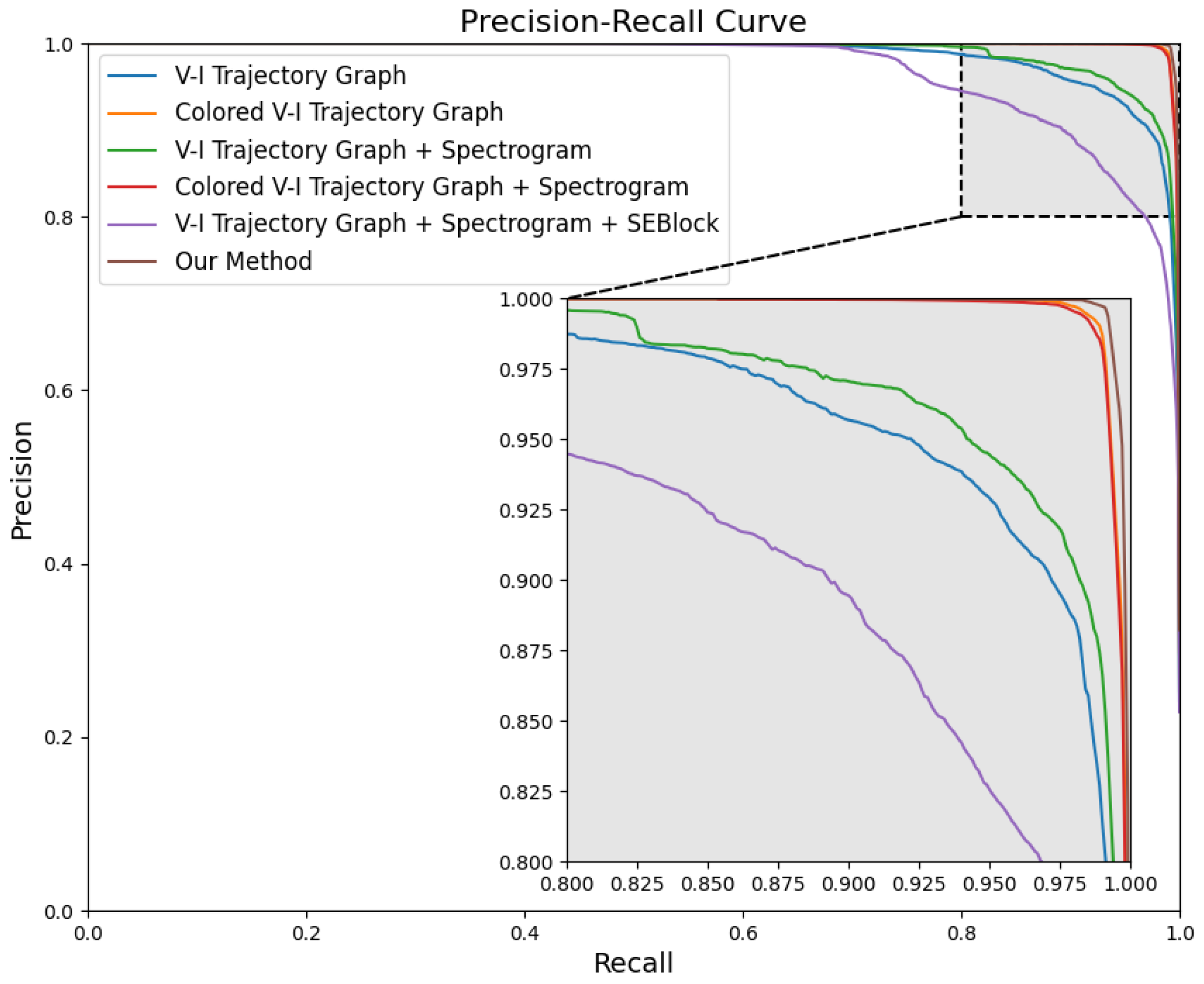
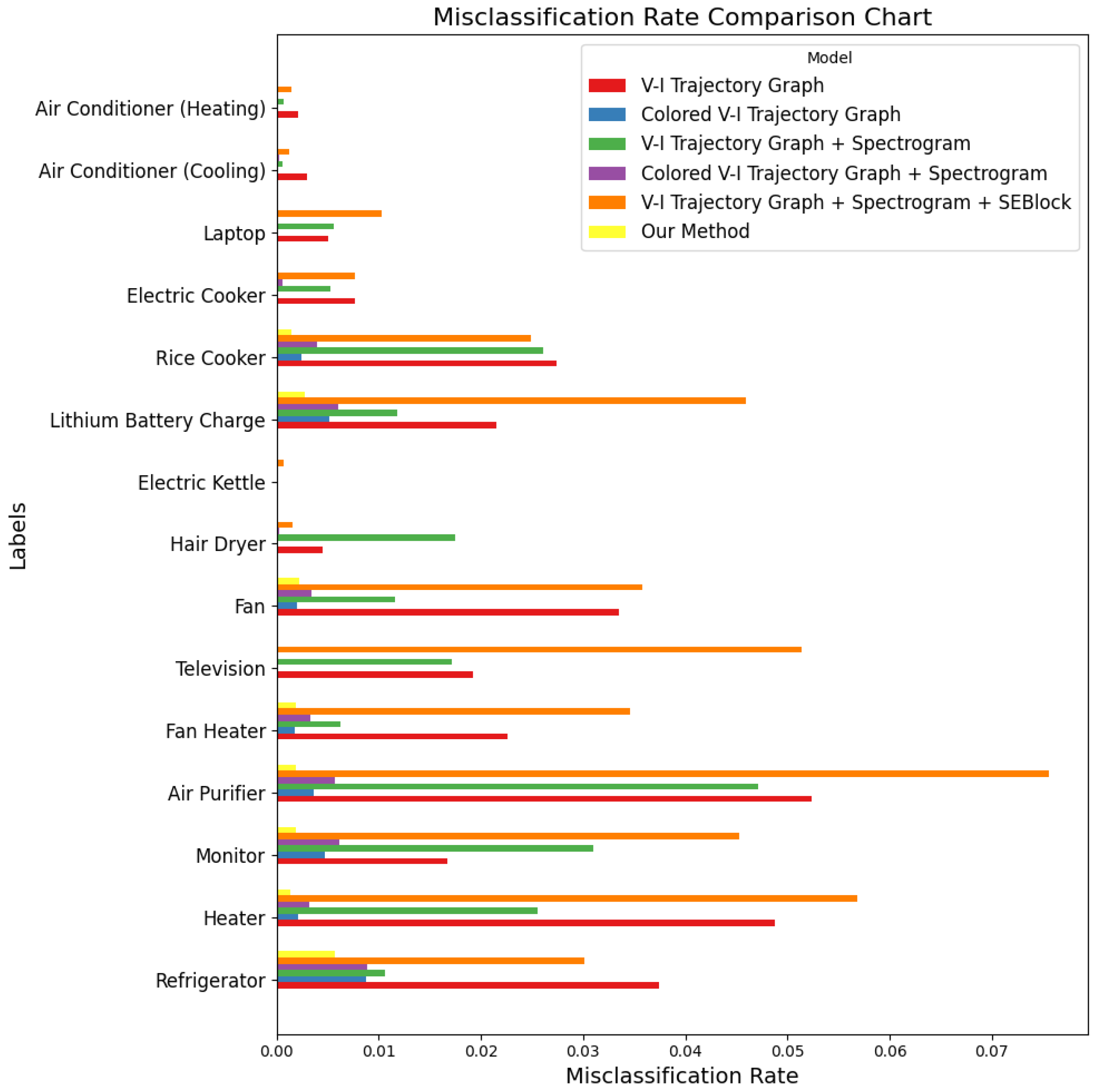
To more intuitively compare the impact of each ablation scheme on performance, the experiment compared the average confusion matrix, precision-recall curve, and misclassification rate diagram of different schemes. 
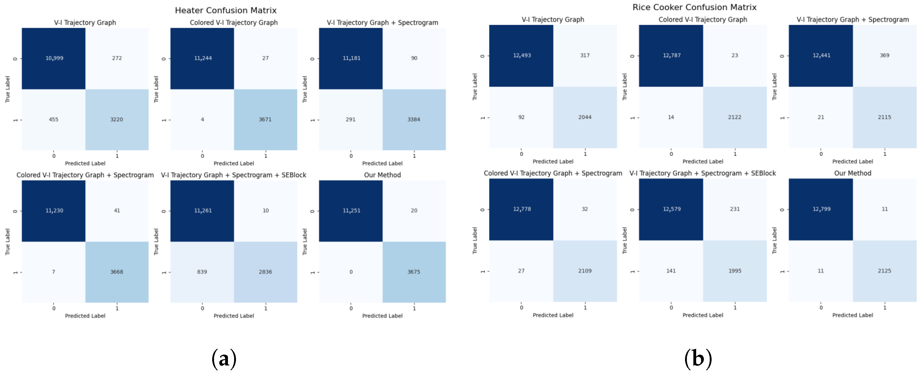
Figure 10 shows the average confusion matrix corresponding to different schemes. It is evident from the figure that as the input features and fusion strategies are gradually optimized, the misclassification phenomenon gradually decreases.
Figure 11 presents the precision-recall curves for each ablation scheme. For precision-recall curves, the larger the area enclosed by the curve and the coordinate axes, the better the performance. From the performance of the curves, it can be seen that our method has the largest curve area, indicating the best performance, which proves the effectiveness of our method.
Figure 12 shows a comparison of misclassification rates for different ablation schemes. It is evident that our method has the lowest misclassification rate across various appliance categories, significantly outperforming the other ablation schemes, further demonstrating the effectiveness of our method.
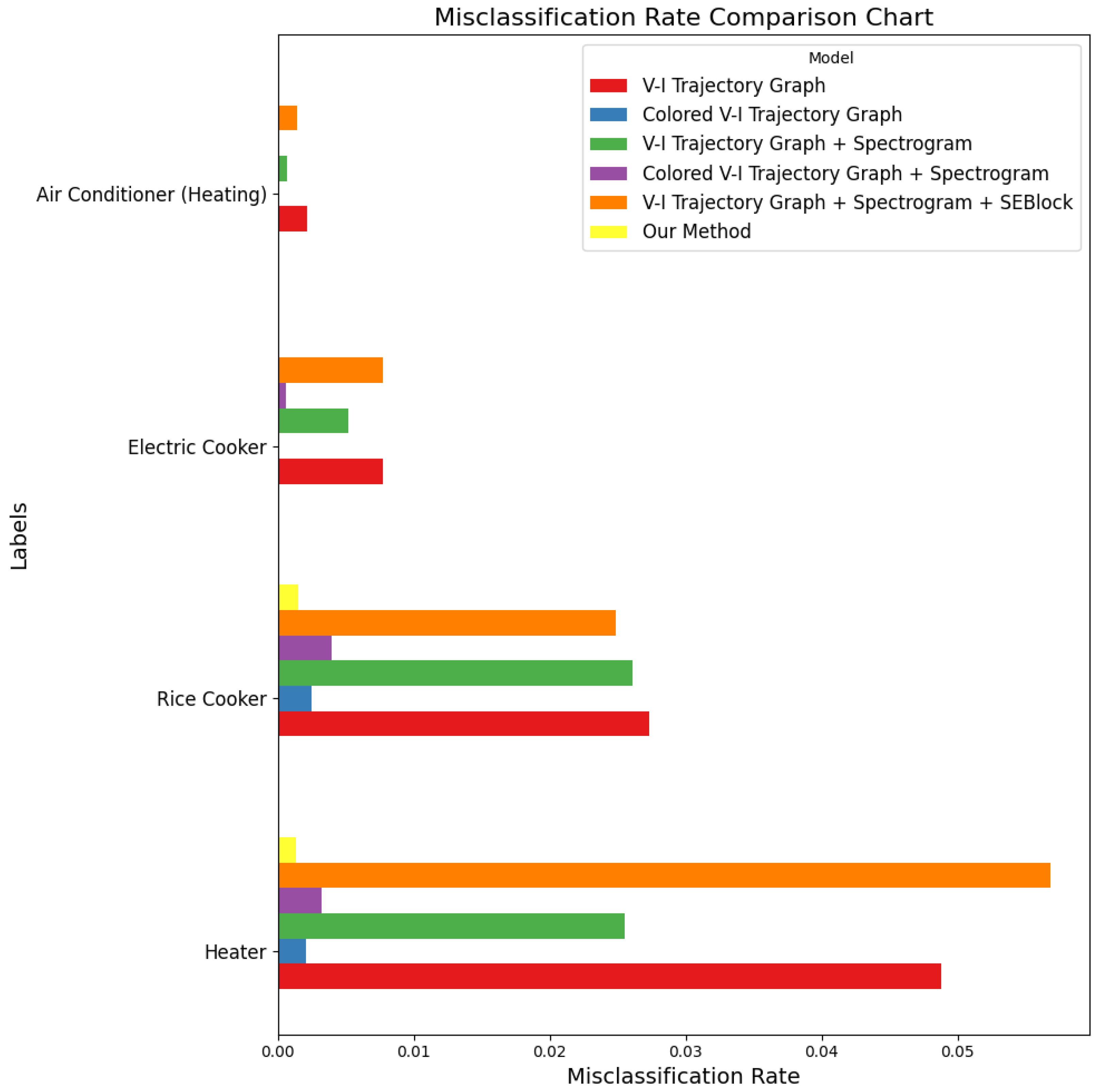
To further evaluate the effectiveness of our method in classifying devices with similar load characteristics, an ablation analysis was conducted on heat-generating appliances—electric heaters (Category 1), rice cookers (Category 10), electric steamers (Category 11), and air conditioning heating (Category 14). The impact of different feature inputs and feature fusion methods on classification performance was observed. The experiment used three metrics: precision, recall, and F1 score. The results are shown in Table 6.
Figure 13, Figure 14, Figure 15 and Figure 16 further demonstrate the performance of each ablation scheme on these heating appliances. Through these charts, the classification capabilities of each method can be seen more clearly.
It can be seen that when only using the V–I trajectory as input, some appliances with similar power consumption patterns (such as rice cookers and electric heaters) exhibit confusion, and their F1 Macro score is significantly lower than other categories. This indicates that relying solely on the features provided by the V–I trajectory is insufficient to accurately distinguish appliances with similar power consumption and the same load type. After using the colored V–I trajectory as a feature expression method, it can be observed that the classification performance has significantly improved compared to the V–I trajectory. The recall rate for rice cookers increased from 98.50% to 99.34%, and the F1 Macro score also increased to 99.14%, with the classification performance of air conditioning reaching the best level. This demonstrates that after adding power consumption features, the colored V–I trajectory has improved the model’s ability to distinguish similar loads, proving the effectiveness of this contribution.
After adding the frequency spectrum as the second input to the model, the results were consistent with the overall ablation experimental results, and the model’s performance on each category fluctuated. The F1 Macro score for rice cookers dropped to 96.77%, and the recall rate also decreased to 98.92%. The recall rate for electric kettles dropped significantly to only 82.48%. This was also due to the interference caused by the direct integration of features of two different types. When using the colored V–I trajectory and frequency spectrum as model inputs, although the overall classification performance improved compared to the traditional V–I trajectory combined with the frequency spectrum, there was still a slight decrease in performance compared to using only the colored V–I trajectory.
After the inclusion of the SE module, the performance of the schemes using frequency spectrum diagrams compared to those not using them showed a certain improvement, which verified the effectiveness of frequency spectrum diagrams in enhancing the classification performance of appliances with similar load characteristics. Moreover, after adding SEBlock, the performance of the schemes compared to direct integration showed a significant improvement, proving the effectiveness of SEBlock in dynamically adjusting feature weights.
The results of the above ablation experiments indicate that for this method, using colored V–I trajectories, introducing frequency spectrum diagrams as secondary input features, and dynamically adjusting each feature weight through the SE module improves the model’s performance in load classification tasks and verifies the effectiveness of each contribution.
To further verify the effectiveness of this method, a comparison was made with traditional deep learning models. The same dataset and evaluation metrics were used, and the input features of the traditional models all used colored V–I trajectories. The evaluation metrics included precision (Precision), recall (Recall), specificity (Specificity), accuracy (Accuracy), and F1 Macro score. For the detailed experimental results, see Table 7.
Figure 17, Figure 18 and Figure 19 represent the average confusion matrix, precision-recall curve, and misclassification rate curve for different models, respectively. Through these figures, the differences in classification performance between different models can be more intuitively observed.
From the results, it can be seen that ResNet10, as a lightweight network, still has certain applicability for processing V–I trajectory images, which are not very complex in terms of features, and has relatively good classification performance, with an F1 Macro score reaching 97.16%. Although its overall performance is not advantageous compared to other models, especially the relatively low accuracy (only 92.27%), the misclassification rate chart shows that the misclassification rate of the ResNet10 model is generally at a lower level across all categories, except for air purifiers. This indicates that it can extract features needed for appliance classification relatively well, but compared to our method, there is still a significant performance gap.
After further increasing the network depth, the performance of ResNet18 compared to ResNet10 improved, with the F1 Macro score increased to 98.99%, and the misclassification rates for all categories decreased compared to ResNet10.
For the ResNet50 and DenseNet121 networks with a larger number of parameters, the additional parameters did not bring significant performance improvements. On the contrary, the precision rate of DenseNet121 is lower than that of ResNet18, and its precision-recall curve is the worst among all methods. Despite having a relatively high F1 Macro score of 99.59% (second only to our method), even ResNet50 has high misclassification rates across all categories, indicating that an excessive number of parameters in V–I trajectory identification can lead to overfitting.
VGG16 and GoogLeNet, as classic convolutional neural network models, also perform well in tasks that require the extraction of multi-scale features from V–I trajectory images. Benefiting from the depth of VGG16, it has outstanding performance in terms of accuracy and specificity, with a specificity of 99.96%, but its F1 Macro of 99.18% is slightly lower than other models, indicating a certain disadvantage compared to our method. GoogLeNet, with the help of Inception modules, provides multi-scale feature extraction capabilities, achieving a recall rate of 99.46%, and its F1 Macro of 99.58% is only slightly lower than the 99.59% value of ResNet50. It also shows good performance in misclassification rate charts, second only to our method.
Finally, our method, by incorporating power-mapped colored V–I trajectory images and combining them with the proposed FD-2DCNN model, integrates V–I trajectory feature extraction modules and frequency domain feature extraction modules. By introducing an attention mechanism, the overall performance is optimized. It can be seen that our method leads other models in terms of precision, recall, and F1 Macro, and it also has the best performance in misclassification rates across all categories, verifying its superiority and reliability in classification tasks.
This chapter proposes a non-intrusive load monitoring method based on power-mapped colored voltage–current (V–I) trajectory diagrams. By adding a method of color mapping based on the magnitude of instantaneous power to the traditional V–I trajectory diagrams, the feature expression is enhanced. Additionally, spectrum diagrams and channel attention mechanisms are incorporated to further improve the richness and expression of features, thereby enhancing recognition performance. In response to the shortcomings of existing public datasets, a high-frequency household appliance current voltage dataset was constructed, and experiments were conducted on this dataset, verifying the method’s advantage in classifying appliances with similar load characteristics.
The FD-2DCNN model demonstrates outstanding performance in 15 appliance classification tasks, achieving an F1 score of 99.67%, significantly outperforming the general image classification performance of ResNet and GoogLeNet in the literature. The reasons for this are as follows: first, it employs dual-modal inputs (128 × 128 × 3 color V–I trajectory images and 128 × 128 × 1 spectrograms), integrating both time-domain and frequency-domain features. Compared to the single-image inputs used by ResNet and GoogLeNet, this approach enables a more comprehensive capture of the electrical characteristics of appliances. Second, the channel attention mechanism (SE module) dynamically adjusts the weights of time-domain and frequency-domain features, optimizing feature fusion. In contrast, the residual connections ResNet and the Inception module of GoogLeNet are primarily designed for general image features and lack targeted optimization for NILM-specific electrical features. Finally, FD-2DCNN, combined with bilinear interpolation preprocessing to ensure high-quality inputs, strikes a balance between computational efficiency and performance. Therefore, through customized dual-modal feature extraction and attention mechanisms, FD-2DCNN significantly enhances classification accuracy and robustness in NILM tasks, surpassing traditional models such as ResNet and GoogLeNet.

5. Conclusions

This study presents a novel NILM method that integrates power-mapped, color-coded voltage–current trajectories with frequency-domain features to achieve robust and precise appliance classification. By developing a high-sampling-rate dataset tailored to modern household appliances and regional grid standards (220 V/50 Hz), we address the limitations of outdated public datasets, ensuring relevance to contemporary smart home ecosystems. The proposed Deep Fusion Two-Dimensional Convolutional Neural Network, augmented by a channel-wise attention mechanism, seamlessly fuses spatial, color, and spectral information, enabling accurate differentiation of appliances with similar load profiles, including resistive and multi-state loads. Comparative experiments and ablation studies confirm the pivotal roles of color mapping, frequency-domain inputs, and attention mechanisms in enhancing classification performance. With efficient inference capabilities suitable for edge deployment, this method offers a scalable solution for advanced household energy monitoring, fostering user-centric energy management and electrical safety.
Looking ahead, future work will scale this approach for real-world smart home applications by expanding the dataset to encompass emerging IoT-enabled appliances and optimizing FD-2DCNN for resource-constrained devices. Integrating transfer learning will enhance adaptability across diverse electrical environments, while real-time anomaly detection will empower users with proactive feedback, strengthening human–computer interaction. Additionally, exploring the role of NILM in promoting energy-conscious behaviors and supporting smart grid policies will advance social informatics, contributing to sustainable energy ecosystems and user-empowered smart communities.

Author Contributions

Conceptualization, X.L. and Y.C.; methodology, Y.C. and S.H.; software, X.J., F.S. and B.S.; validation, X.L. and J.G.; formal analysis, X.L. and S.H.; investigation, X.L.; resources, X.L.; data curation, Y.C.; writing—original draft preparation, Y.C.; writing—review and editing, J.G.; visualization, X.J., F.S. and B.S.; supervision, X.L.; project administration, X.L.; funding acquisition, X.L. All authors have read and agreed to the published version of the manuscript.

Funding

This research was substantially supported by Major Project in Humanities and Social Sciences of Tianjin Municipal Education Commission: Research on Big Data Activating the Cultural New Momentum of Tianjin’s ‘Grand Canal+’ Initiative. Project Number: No.2021JWZD11.

Institutional Review Board Statement

Not applicable.

Informed Consent Statement

Not applicable.

Data Availability Statement

The data presented in this study are available upon request from the corresponding author. The data are not publicly available, as they are related to our subsequent research.

Conflicts of Interest

The authors declare no conflicts of interest.

References

  1. Zeng, W.; Han, Z.; Xie, Y.; Liang, R.; Bao, Y. Non-intrusive load monitoring through coupling sequence matrix reconstruction and cross stage partial network. Measurement 2023, 220, 113358. [Google Scholar] [CrossRef]
  2. Zheng, G.; Hu, Y.; Xiao, Z.; Ding, X. Graph-Based Dependency-Aware Non-Intrusive Load Monitoring. In Proceedings of the Chinese Conference on Pattern Recognition and Computer Vision (PRCV), Xiamen, China, 13–15 October 2023; pp. 89–100. [Google Scholar]
  3. Zhou, K.; Zhang, Z.; Lu, X. Non-intrusive load monitoring based on an efficient deep learning model with local feature extraction. IEEE Trans. Ind. Inform. 2024, 20, 9497–9507. [Google Scholar] [CrossRef]
  4. Yan, Z.; Hao, P.; Nardello, M.; Brunelli, D.; Wen, H. A Generalizable Load Recognition Method in NILM Based on Transferable Random Forest. IEEE Trans. Instrum. Meas. 2025, 74, 6505312. [Google Scholar] [CrossRef]
  5. de Diego-Otón, L.; Hernández, Á.; Fuentes, D.; Nieto, R.; Navarro, V.M. Architectural strategies for enhanced NILM classification and anomaly detection: Addressing limited data scenarios. Expert Syst. Appl. 2025, 282, 127756. [Google Scholar] [CrossRef]
  6. Hao, P.; Yan, Z.; Wen, H. Privacy-Preserving NILM: A Self-Alignment Source-Aware Domain Adaptation Approach. IEEE Trans. Instrum. Meas. 2025, 74, 2507612. [Google Scholar] [CrossRef]
  7. Shi, D. NILM Datasets for Research: IAWE, REDD, and UKDALE. IEEE Dataport. 2024. Available online: https://ieee-dataport.org/documents/nilm-datasets-research-iawe-redd-and-ukdale (accessed on 12 June 2025).
  8. Guo, X.; Wang, C.; Wu, T.; Li, R.; Zhu, H.; Zhang, H. Detecting the novel appliance in non-intrusive load monitoring. Appl. Energy 2023, 343, 121193. [Google Scholar] [CrossRef]
  9. Chen, C.; Gao, P.; Jiang, J.; Wang, H.; Li, P.; Wan, S. A deep learning based non-intrusive household load identification for smart grid in China. Comput. Commun. 2021, 177, 176–184. [Google Scholar] [CrossRef]
  10. Lu, J.; Zhao, R.; Liu, B.; Yu, Z.; Zhang, J.; Xu, Z. An overview of non-intrusive load monitoring based on VI trajectory signature. Energies 2023, 16, 939. [Google Scholar]
  11. Shi, J.; Zhi, D.; Fu, R. Research on a non-intrusive load recognition algorithm based on high-frequency signal decomposition with improved VI trajectory and background color coding. Mathematics 2023, 12, 30. [Google Scholar] [CrossRef]
  12. Han, Y.; Li, K.; Feng, H.; Zhao, Q. Non-intrusive load monitoring based on semi-supervised smooth teacher graph learning with voltage–current trajectory. Neural Comput. Appl. 2022, 34, 19147–19160. [Google Scholar] [CrossRef]
  13. Chen, T.; Qin, H.; Li, X.; Wan, W.; Yan, W. A non-intrusive load monitoring method based on feature fusion and SE-ResNet. Electronics 2023, 12, 1909. [Google Scholar] [CrossRef]
  14. Grover, H.; Panwar, L.; Verma, A.; Panigrahi, B.K.; Bhatti, T. A multi-head Convolutional Neural Network based non-intrusive load monitoring algorithm under dynamic grid voltage conditions. Sustain. Energy Grids Netw. 2022, 32, 100938. [Google Scholar] [CrossRef]
  15. Yao, L.; Wang, J.; Zhao, C. Non-Intrusive Load Monitoring Based on Multiscale Attention Mechanisms. Energies 2024, 17, 1944. [Google Scholar] [CrossRef]
  16. Xiang, Y.; Ding, Y.; Luo, Q.; Wang, P.; Li, Q.; Liu, H.; Fang, K.; Cheng, H. Non-invasive load identification algorithm based on color coding and feature fusion of power and current. Front. Energy Res. 2022, 10, 899669. [Google Scholar] [CrossRef]
  17. He, J.; Liu, J.; Zhang, Z.; Chen, Y.; Liu, Y.; Khoussainov, B.; Zhu, L. MSDC: Exploiting multi-state power consumption in non-intrusive load monitoring based on a dual-CNN model. In Proceedings of the AAAI Conference on Artificial Intelligence, Washington, DC, USA, 7–14 February 2023; Volume 37, pp. 5078–5086. [Google Scholar]
  18. Liu, H.; Sun, Y.; Wang, Y. A Non-Invasive Load Monitoring Method for Edge Computing Based on MobileNetV3 and Dynamic Time Regulation. arXiv 2025, arXiv:2504.16142. [Google Scholar]
  19. Sykiotis, S.; Athanasoulias, S.; Kaselimi, M.; Doulamis, A.; Doulamis, N.; Stankovic, L.; Stankovic, V. Performance-aware NILM model optimization for edge deployment. IEEE Trans. Green Commun. Netw. 2023, 7, 1434–1446. [Google Scholar] [CrossRef]
  20. Wang, J.; Pang, C.; Zeng, X.; Chen, Y. Non-intrusive load monitoring based on residual u-net and conditional generation adversarial networks. IEEE Access 2023, 11, 77441–77451. [Google Scholar] [CrossRef]
  21. Azad, M.I.; Rajabi, R.; Estebsari, A. Non-intrusive load monitoring (nilm) using deep neural networks: A review. In Proceedings of the 2023 IEEE International Conference on Environment and Electrical Engineering and 2023 IEEE Industrial and Commercial Power Systems Europe (EEEIC/I&CPS Europe), Madrid, Spain, 6–9 June 2023; pp. 1–6. [Google Scholar]
Figure 1. Color-coded voltage and current trajectory diagrams based on power mapping.
Informatics 12 00055 g001
Figure 2. Color-coded voltage and current trajectory diagrams based on power mapping.
Informatics 12 00055 g002
Figure 3. FD-2DCNN model architecture diagram.
Informatics 12 00055 g003
Figure 4. Feature extraction module model.
Informatics 12 00055 g004
Figure 5. (a) Current waveform before denoising. (b) Current waveform after denoising. (c) Colored V–I trajectory diagrams without denoising (d) Colored V–I trajectory diagrams with denoising.
Informatics 12 00055 g005
Figure 6. (a) Scaled color V–I trajectory plot. (b) Scaled FFT spectrum plot.
Informatics 12 00055 g006
Figure 7. Model multi-label classification result confusion matrix.
Informatics 12 00055 g007
Figure 8. Model precision-recall curve.
Informatics 12 00055 g008
Figure 9. Model misclassification rate chart for different electrical appliances.
Informatics 12 00055 g009
Figure 10. Average confusion matrix for different schemes.
Informatics 12 00055 g010
Figure 11. Precision-recall curves for different schemes.
Informatics 12 00055 g011
Figure 12. Comparison chart of misclassification rates for different schemes.
Informatics 12 00055 g012
Figure 13. (a) Electric Heater ablation experiment confusion matrix. (b) Rice Cooker ablation experiment confusion matrix.
Informatics 12 00055 g013
Figure 14. (a) Electric Cooker ablation experiment confusion matrix. (b) Air Conditioner heating ablation experiment confusion matrix.
Informatics 12 00055 g014
Figure 15. (a) Precision-recall curves of Electric Heater ablation experiments. (b) Air Conditioner heating ablation experiment confusion matrix. (c) Precision-recall curves for Electric Cooker ablation experiments. (d) Precision-recall curves for Air Conditioner heating ablation experiments.
Informatics 12 00055 g015
Figure 16. Misclassification rate chart for ablation experiments on four types of heating appliances.
Informatics 12 00055 g016
Figure 17. Confusion matrices for different models.
Informatics 12 00055 g017
Figure 18. Precision-recall curves for different models.
Informatics 12 00055 g018
Figure 19. Misclassification situations for different models.
Informatics 12 00055 g019
Table 1. Appliance categories.
IndexAppliance Category
0Refrigerator
1Heater
2Computer Monitor
3Air Purifier
4Heater
5Television
6Electric Fan
7Hair Dryer
8Electric Kettle
9Electric Vehicle Battery Charging
10Rice Cooker
11Electric Cooker
12Laptop Computer
13Air Conditioning Cooling
14Air Conditioning Heating
Table 2. Hardware parameters.
HardwareDetails
Epochs50
OptimizerAdam
Learning Rate0.01
Batch Size32
Table 3. Hardware parameters.
HardwareDetails
CPUAMD Ryzen9 5900 4.2Ghz (Santa Clara, CA, USA)
RAM32GB DDR4
GPUNvidia GeForce RTX 3090 (Santa Clara, CA, USA)
vRAM24GB
Table 4. Experimental results.
Precision (%)Recall (%)Specificity (%)Accuracy (%)F1 Macro (%)Average Time (ms)
99.8599.5099.9598.9899.670.88
Table 5. Overall ablation experiment results.
MethodPrecision (%)Recall (%)Specificity (%)Accuracy (%)F1 Macro (%)
V–I Trajectory Map99.4098.9599.8797.6799.17
Color V–I Trajectory Map99.6799.4299.9098.2199.54
V–I Trajectory Map + Spectrum Map98.2798.1399.7897.6498.13
Color V–I Trajectory Map + Spectrum Map99.3899.0399.8797.8399.20
V–I Trajectory Map + Spectrum Map + SEBlock99.4099.1099.8898.1799.25
Our Method99.8599.5099.9598.9899.67
Table 6. Ablation test results for heating appliances.
MethodAppliance TypePrecision (%)Recall (%)F1 (%)
V–I TrajectoryElectric Heater98.8699.4899.17
Rice Cooker98.3698.5098.43
Electric Kettle99.9997.1498.01
Air Conditioner97.5299.1698.33
Colored V–I TrajectoryElectric Heater99.2799.8999.58
Rice Cooker98.9399.3499.14
Electric Kettle99.9999.9999.99
Air Conditioner99.9999.9999.99
V–I Trajectory + FrequencyElectric Heater99.2799.4699.36
Rice Cooker94.7198.9296.77
Electric Kettle97.1582.4889.22
Air Conditioner99.1799.9999.58
Colored V–I Trajectory + FrequencyElectric Heater98.8999.8199.35
Rice Cooker98.5198.7498.62
Electric Kettle97.6399.7098.65
Air Conditioner99.9999.9999.99
V–I Trajectory + Frequency + SEBlockElectric Heater99.1399.5999.36
Rice Cooker98.7898.8398.81
Electric Kettle99.3897.5898.48
Air Conditioner99.1699.1699.16
Our MethodElectric Heater99.4699.9999.73
Rice Cooker99.4999.4999.49
Electric Kettle99.9999.9999.99
Air Conditioner99.9999.1699.58
Table 7. Model comparison results.
MethodPrecision (%)Recall (%)Specificity (%)Accuracy (%)F1 Macro (%)
ResNet1096.2898.4399.8492.2797.16
ResNet1899.2599.7899.9497.6298.99
ResNet5099.4999.7099.9699.0099.59
DenseNet12199.1297.8199.8194.3198.35
VGG1699.4498.9499.9698.7199.18
GoogLeNet99.7199.4699.9498.6899.58
Our Method (FD-2DCNN)99.8599.5099.9598.9899.67
Disclaimer/Publisher’s Note: The statements, opinions and data contained in all publications are solely those of the individual author(s) and contributor(s) and not of MDPI and/or the editor(s). MDPI and/or the editor(s) disclaim responsibility for any injury to people or property resulting from any ideas, methods, instructions or products referred to in the content.

