Abstract
Survival analysis is a crucial statistical technique used to estimate the anticipated duration until a specific event occurs. However, current methods often involve discretizing the time scale and struggle with managing absent features within the data. This becomes especially pertinent since events can transpire at any given point, rendering event analysis a continuous concern. Additionally, the presence of missing attributes within tabular data is widespread. By leveraging recent developments of Transformer and Self-Supervised Learning (SSL), we introduce SSL-SurvFormer. This entails a continuously monotonic Transformer network, empowered by SSL pre-training, that is designed to address the challenges presented by continuous events and absent features in survival prediction. Our proposed continuously monotonic Transformer model facilitates accurate estimation of survival probabilities, thereby bypassing the need for temporal discretization. Additionally, our SSL pre-training strategy incorporates data transformation to adeptly manage missing information. The SSL pre-training encompasses two tasks: mask prediction, which identifies positions of absent features, and reconstruction, which endeavors to recover absent elements based on observed ones. Our empirical evaluations conducted across a variety of datasets, including FLCHAIN, METABRIC, and SUPPORT, consistently highlight the superior performance of SSL-SurvFormer in comparison to existing methods. Additionally, SSL-SurvFormer demonstrates effectiveness in handling missing values, a critical aspect often encountered in real-world datasets.
1. Introduction
Survival analysis or time-to-event analysis is a fundamental area of statistics concerned with estimating the time until an event occurs, such as a death in biological organisms [1] and failure in mechanical systems [2]. In this paper, we focus on survival regression, which is a type of analysis that relates the time until an event occurs to one or more covariates that may be associated with that duration of time. Censoring is a common issue in survival analysis where events are not always fully observed, often due to limited observation time windows or missing data. We specifically consider right-censored data, where the event is known to have occurred after a certain time but not precisely when. Examples of applications that employ right-censored data include medical treatment recovery time [3], business prediction [4], and churn prediction [5].
Traditional approaches to survival analysis, such as the Kaplan–Meier [6] estimator, the Cox proportional hazard model [7], and the accelerated failure time method [8], were popular before the advent of machine learning. In recent years, machine learning methods, including support vector machines [9,10], random survival forests (RSFs) [11], and gradient boosting [12], have been proposed for survival analysis. Deep learning models like SuMo-Net [13], DeepHit [14], and DeepSurv [15] have advanced survival analysis through neural networks. However, these approaches face significant limitations. Most rely on basic MLP architectures that struggle to capture complex interactions between features. Additionally, many methods (including DeepHit [14], SurvTRACE [16], and TransDSA [17]) discretize continuous survival time into intervals, resulting in information loss.
Transformer, a highly effective sequence modeling architecture, has demonstrated state-of-the-art (SOTA) performance in various applications, including natural language processing (NLP) [18,19,20], speech recognition [21,22], image understanding [23,24,25], and video analysis [26,27]. Recently, Transformer-based methods for tabular data and survival analysis have emerged, including TabTrans [28], FT-Transformer [29], SurvTRACE [16], and TransDSA [17]. According to the published results, these approaches demonstrate superior performance compared to traditional MLP-based methods. Despite these advancements, these models still face the fundamental discretization problem. This issue occurs when continuous survival times must be converted into fixed intervals, introducing several significant limitations: arbitrary interval selection, a trade-off between temporal resolution and data sparsity, and the constraint of predictions to predefined timepoints rather than the full continuous time spectrum.
Another issue in the survival analysis problem is missing features, some of instances in our dataset may have absent features due to various reasons during data collection, processing, storage, or transmission. It is often desirable to know the most likely values of missing data before performing downstream tasks. Existing deep-learning-based methods in survival analysis are not able to handle missing features in survival data. Consequently, they resort to imputation methods like mean/mode imputation and KNN imputation.
In this paper, we address three critical limitations in current survival analysis approaches: (1) discretization of continuous time leading to information loss, (2) architectural constraints of basic MLPs that fail to capture complex feature interactions, and (3) inability to handle missing data without separate imputation steps. We introduce SSL-SurvFormer, which combines a continuously monotonic Transformer architecture with self-supervised learning (SSL) pre-training to overcome these challenges. Our approach enforces positivity constraints on time-related weights, mathematically guaranteeing the monotonicity properties of survival functions without approximation errors. This novel constraint enables direct estimation of the continuous survival function without discretizing time intervals. The model operates in two phases: SSL pre-training with data augmentation followed by fine-tuning of our continuously monotonic Transformer. This integrated approach eliminates the need for separate imputation steps, as missing data handling is directly incorporated into the model. Comprehensive experiments on the FLCHAIN [30], METABRIC [31], and SUPPORT [32] datasets demonstrate that SSL-SurvFormer significantly outperforms existing methods in both prediction accuracy and missing data handling capability. As shown in Table 1, our approach maintains superior performance across datasets with varying levels of missing values, highlighting its robustness and practical utility for real-world survival analysis applications.

Table 1.
Comparison between our proposed SSL-SurvFormer and the existing survival analysis methods. MLP stands for Multilayer Perceptron.
2. Related Work
Traditional Survival Prediction: One of the most common survival models in statistical and medical research is the Kaplan–Meier estimator [6], which benefits from learning relatively flexible survival curves. However, it has the drawback of not taking into account the covariates of the patients. The Cox proportional hazard model [7] is capable of incorporating patients’ covariates, but assumes that the hazard rate is constant and that the log of the hazard rate is a linear function of the covariates.
MLP-based Survival Prediction: With the advancement of neural networks, researchers have explored the application of deep learning networks in the field of survival analysis. The Multilayer Perceptron (MLP) [33], a foundational neural network architecture consisting of an input layer, hidden layers with non-linear activation functions, and an output layer, has been widely used for its ability to model complex patterns. MLPs were among the first deep learning approaches applied to survival analysis. By replacing the linear function in Cox model with a MLP, ref. [15] proposed DeepSurv, which is also optimized the model’s partial log-likelihood. However, this approach relies on the same proportional hazards assumption of Cox’s method, which difficult to verify or need to check very carefully every time in medical application. To overcome this issue, ref. [14] introduced DeepHit, which divides the timescale into discrete intervals, then the model is trained by optimizing a mix of the discrete likelihood and a rank-based score. The task becomes similar to a classification in which each outcome is a binary variable reflecting if the patient survives within a specific time interval. As a non-parametric model, this approach offers better discriminative performances when the underlying survival distribution is unknown. However, it suffers from its discretization i.e., determining the breakpoints for time intervals is non-trivial, since too many intervals may lead to unstable model estimation while too few intervals may cause information loss. Furthermore, since the model is optimized for a fixed set of output timepoints, it may not be adaptable for making inferences on other timepoints. There are some attempts to surpass the limitations of timescale discretization. Refs. [34,35] use Ordinary Differential Equations (ODEs) to parameterize the cumulative hazard function, while ref. [36] uses ODEs to parameterize the cumulative distribution function. Closer to our work, ref. [13] described another neural network that avoids the computational burden of ODE, which is a simple MLP survival model capable of directly modeling survival data continuously using a monotonic restriction on the time-dependent weight. While NeuralODEs represent a powerful modeling paradigm for survival analysis, they suffer from significant computational limitations in practical applications. As demonstrated by [37,38], NeuralODEs exhibit computational complexity that grows polynomially with the number of parameters, primarily due to their reliance on numerical ODE solvers that require multiple function evaluations per forward pass. In contrast, our monotonically positive component maintains linear scaling characteristics similar to standard neural networks, offering substantially improved computational efficiency for larger models. Furthermore, by enforcing strict positivity constraints on time-related weights, our approach provides mathematical guarantees of monotonicity for survival functions without introducing the approximation errors inherent in numerical ODE solutions. This mathematical guarantee eliminates potential instabilities and ensures that our model’s outputs consistently satisfy the fundamental monotonicity property required for valid survival function estimation, regardless of parameter initialization or training dynamics. Besides, the deep learning-based models mentioned earlier primarily rely on MLP networks, making them incapable of directly addressing missing values in the dataset.
Transformer-based Survival Prediction: Transformer was first introduced in [39] for language translation and obtained state-of-the-art (SOTA) results in many other language processing tasks. Recently, many models [40,41,42] have successfully applied the Transformer concept to computer vision and tabular data and achieved promising performance. The core idea behind transformer architecture [39] is the self-attention mechanism to capture long-range relationships. It has obtained state-of-the-art in many Natural Language Processing (NLP) tasks. Moreover, Transformers are well suited for parallelization, facilitating training on large datasets. In survival analysis, TransDSA [17] and SurvTRACE [16] utilize Transformer instead of an MLP to better learn survival distribution, model long-range coherence, and obtain higher performance. TransDSA [17] proposed using a Transformer network along with time embeddings, but they treated numerical and categorical data using a single network. On the other hand, SurvTRACE [16] also employed the Transformer architecture but had separate embedding modules for these two types of features, resulting in improved performance. However, they have shared the same discrete time approach with DeepHit [14], dividing the time scale into intervals. This approach posed a common challenge in selecting the appropriate interval. Additionally, neither of these methods offered a solution for handling missing data, requiring the imputation of missing values before training the models.
Handling missing features in survival data: There are several approaches to handling missing data, broadly categorized into deletion and imputation methods. In deletion, entries with missing values are discarded, and this can be performed through pairwise or list-wise deletion [43]. However, as demonstrated in [44], deletion has some weaknesses, as it can introduce bias. On the other hand, imputation involves replacing missing values with predicted values, as outlined in [43]. In simple imputation, missing data can be handled using various methods, including the mode, mean, or median of the available values [45]. Mean imputation is commonly used for numerical data, while mode imputation is typically applied to categorical data. In mode imputation, the mode of an attribute is used to impute the missing value for the corresponding attribute.
A more advanced approach is K-nearest neighbor (KNN) imputation, which use Euclidean distance to impute the missing features using the closest samples. In the era of deep learning (DL), generative models have been utilized to address missing values. For instance, in [46], a GAN-based model is employed to generate synthetic values for the missing data, leveraging the information from the observed values. Similarly, [47] suggested using a generative model, specifically the Variational Autoencoder (VAE) model, to perform the imputation of missing values. Generative approaches for handling missing values typically involve a two-step process. In the first step, a dedicated model is trained for imputation to fill in the missing data; in the second step, a downstream model is trained for the primary task. In this work, we concentrate exclusively on survival analysis tasks involving missing features by leveraging SSL.
3. Proposed Method
3.1. Problem Setup and Notations
Our proposed SSL-SurvFormer aims to model survival prediction in continuous time, thus, we follow the problem setup defined in SuMo-Net [13] as follows. Given a dataset , where Z is the number instances in the dataset and i indicates the ith instance (i.e, patient), each instance in the dataset associates with a set of covariates for , the time when the events occur or the sample is censored , and event censoring or occurrence at time , where means censoring. Let T be a random variable representing time to the event; our work only considers the case in which event time T can be observed or censored (right-censored). Our model objective is to estimate the survival function: , which is defined as a (conditional) survival distribution . In the formula, is the cumulative distribution function (CDF) when assuming event time is a continuous random variable. Moreover, the probability density function (PDF) of T is .
Our goal is summarized as follows: If the survival function of T is denoted by , we aim to predict an estimated distribution using dataset , such as estimated distribution as close as truth distribution S.
We first present a continuously monotonic Transformer for survival analysis, named SurvFormer. We then introduce SSL and integrate into SurvFormer to form SSL-SurvFormer.
3.2. SurvFormer: Network Architecture
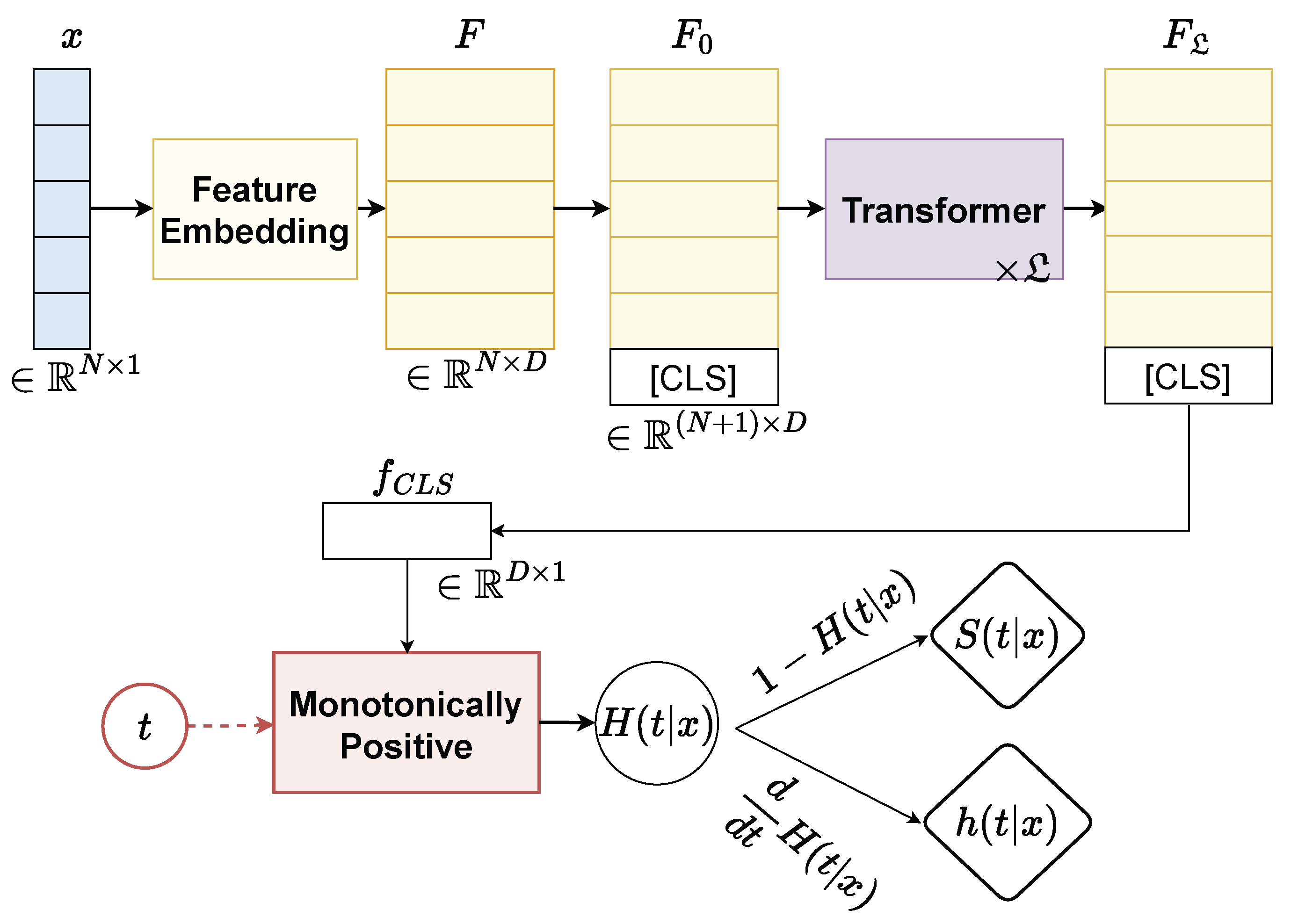
The overall network architecture of our proposed continuously monotonic Transformer, termed SurvFormer, is given in Figure 1. SurvFormer consists of three components including Feature Embedding to extract the feature representation of an instance, Transformer to model the contextual coherence between attributes, and a Monotonically Positive to restrict the monotonicity constraint. Details of each component are as follows:
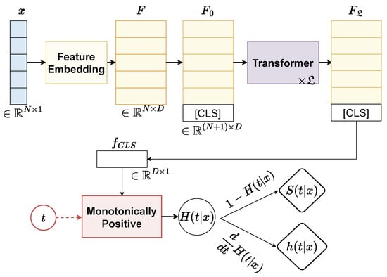
Figure 1.
The overall architecture of our SurvFormer consists of (i) Feature Embedding to the extract feature representation of an instance, (ii) Transformer to model the contextual coherence, and (iii) a monotonically positive component to restrict the network with a monotonicity constraint.
3.2.1. Feature Embedding
For a general instance defined by , its data x can be separated into two types: categorical data and numerical data such as and . We transform the categorical data into numbers and normalize the numerical data and the instance’s time s before feeding the model. We separately process numerical data and categorical data as follows.
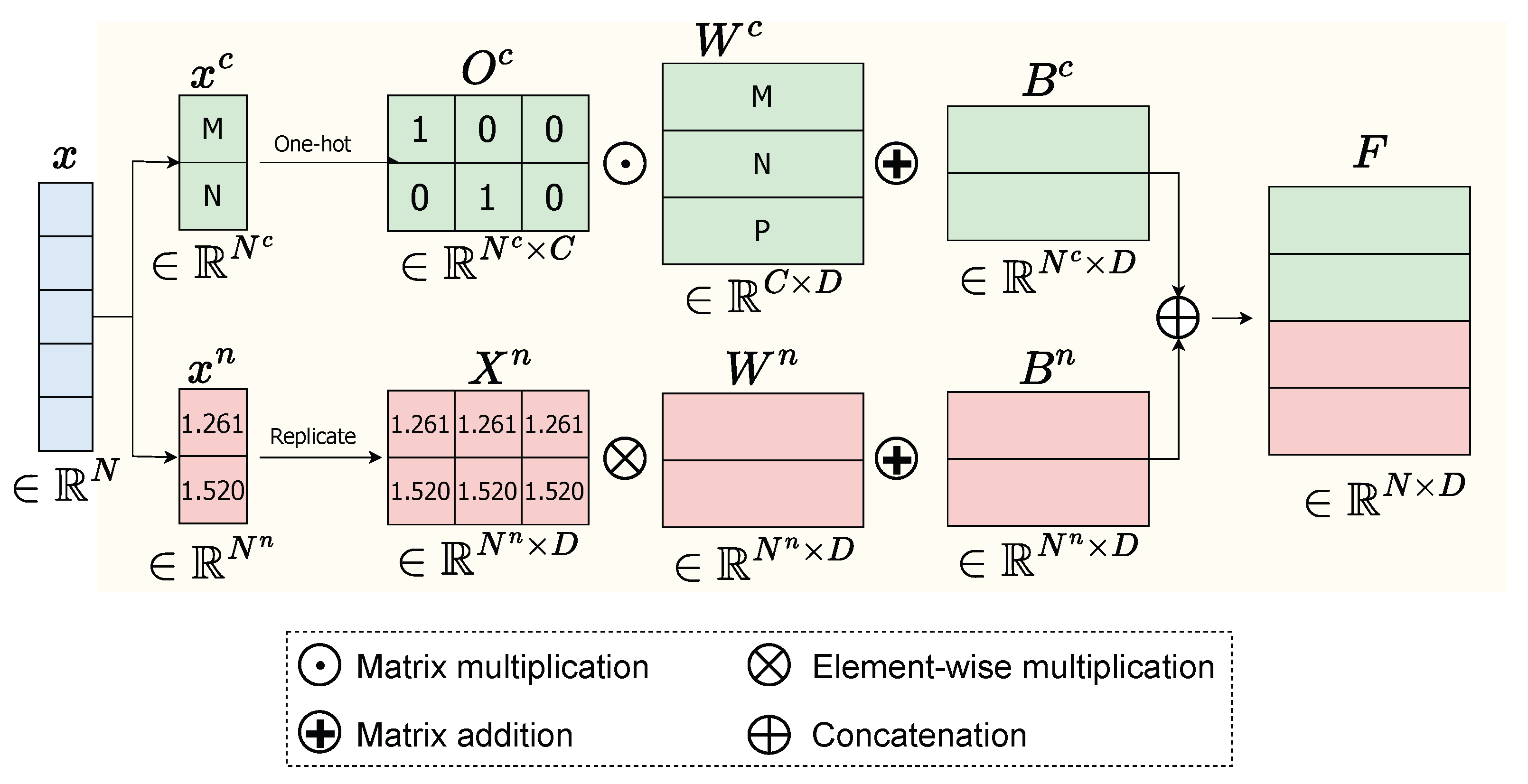
Numerical data: The numerical data is computed by Equation (1).
where is a vector, is the unit vector with D dimensions, is a matrix obtained by replicating the vector D times, ⊙ represents element-wise between and , is the embedding matrix for numerical features, and is bias. The output numerical feature representation will be in dimensional space of .
Categorical data: The categorical data, which is commonly represented by one-hot encoding, is embedded as a lookup table through an embedding matrix , where C is the total number of distinct values in all categorical features. For instance, if a patient record contains two categorical variables—occupation (3 unique values) and gender (2 unique values)—then C = 5. The categorical embedding feature of is computed in Equation (2).
where is the one-hot representation of and is bias.
Finally, we stack both the numerical embedding feature and categorical embedding feature to obtain the final feature representation , where . The flowchart of the Feature Embedding component is demonstrated in Figure 2.
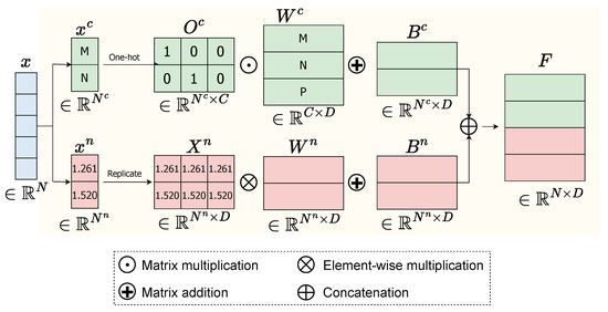
Figure 2.
Flowchart of Feature Embedding of a given data x consisting of categorical data and numerical data .
3.2.2. Transformer
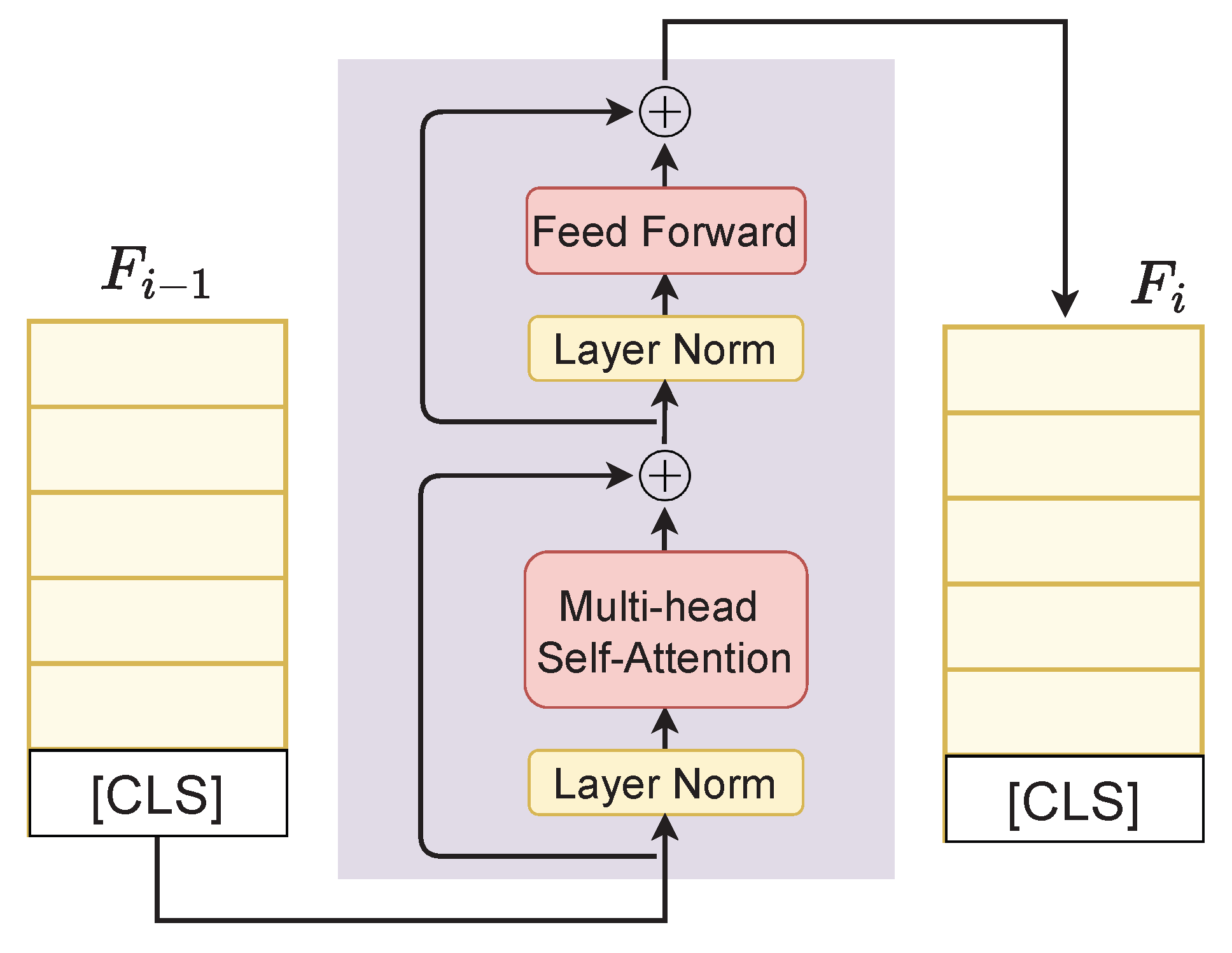
We inherit the merits of PreNorm-variant Transformer architecture defined in [29,48], where the model takes in a sequence of feature embeddings and outputs contextual representations of the same dimension. Following [18], we first append the embeddings of the classification token [CLS] to feature representation F to form a new feature representation . The embedding then goes through a Transformer with blocks and we finally obtain the contextual representation as shown in Figure 1. The detailed network of a Transformer block is given in Figure 3 and the Transformer is described in Algorithm 1.
| Algorithm 1 Transformer |
|
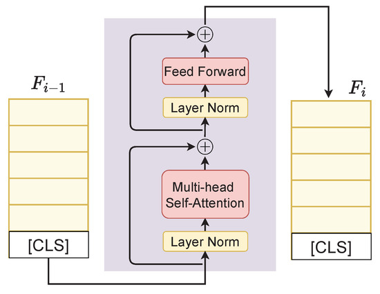
Figure 3.
Details of a Transformer block. is the feature representation at the layer i. ⊕ denotes the addition operation.
In Algorithm 1, FFN and RPN stand for feed-forward network and residual pre-norm module, Norm is LayerNorm [49], and MHSA is multihead self-attention, respectively. We use ReGLU (Regularized Gated Linear Unit) as an activation function due to its reported superiority over the commonly used GELU activation [50,51].
3.2.3. Monotonically Positive
This component aims to restrict the monotonicity constraint and output the estimated survival function. Let denote the survival function, which is defined as in Equation (3)
Survival functions follow these same three characteristics:
- As t increases, should decrease.
- . That is at the start of the study, no one has the event, thus the probability of surviving at is 1.
- . If the study were to go to , then everyone will eventually experience the event and hence the survival probability must be 0.
Inspired by [13,52], our monotonically positive component enforces the network’s weights to be positive to ensure the monotonicity of the survival function. To ensure that the output of the neural network does not decrease as time t increases, we enforce non-negativity constraints on the weights applied to time t.
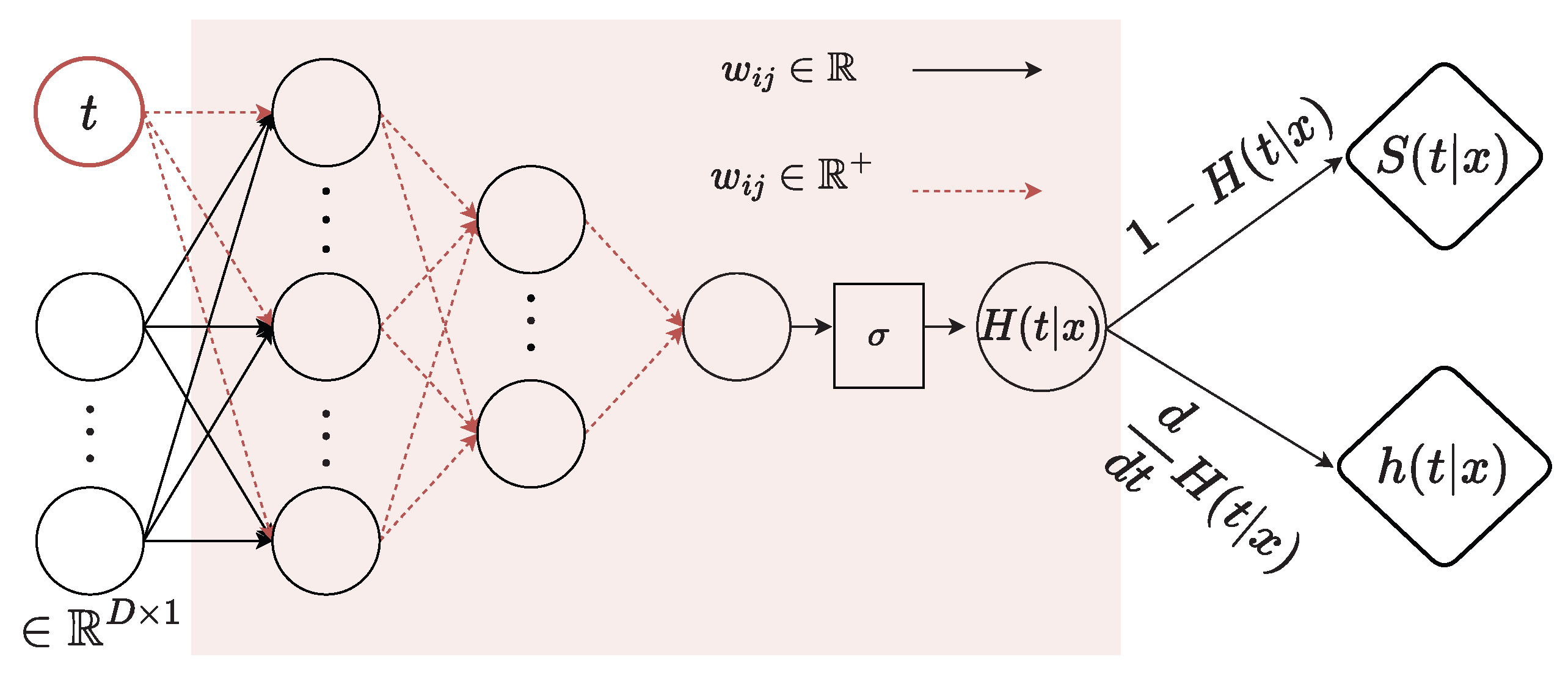
Our monotonically positive component is defined as an MLP with K layers, where tanh is an activation function of layers and sigmoid is an activation function of the last layer. The monotonically positive component takes the last feature representation of , i.e., and time t as input of the first layer . At the first layer , the weights on time input t are required to be positive, while the weights on the embeddings have no constraint. As other layers , all the weights are forced to be positive. We use the log space or the square function as in [13] to guarantee the positivity of weights and the existence of a derivative. In this network, sigmoid is used in the last layer to output a probability-like value, which also is . Finally, the survival probability at time t is equal to the difference of and 1, i.e., . Moreover, another output is the PDF of t, which is obtained by computing the derivative of , i.e., , and is used to compute the loss function in Equation (4). Our monotonically positive network computed the function through feed-forward. After that, we used PyTorch’s autograd [53] to backpropagate to obtain with respect to t. Thus, when the computed gradient of the loss is mentioned, we used autograd again to backpropagate with respect to the model’s weights. Our implementation follows [13]. The entire flowchart of the monotonically positive component is given in Figure 4.
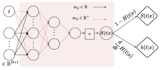
Figure 4.
Details of the monotonically positive component. and are the CDF and PDF, respectively, when assuming event time is a continuous random variable. is the survival function.
3.2.4. Loss Function
Our model aims to optimize the negative log-likelihood loss function for censored data, which is often used to train the survival model. As defined in [13], the right-censored log-likelihood score of a set of observations is calculated as in Equation (4):
Furthermore, we propose to add another loss component , which will penalize the model when its outputs are not in the true order. In this loss , we compare the estimated survival function between two instance and observed at the same time .
where A is the indicator of pair , and are survival functions of two instances at time , and represents the function that determines the magnitude of penalization the model incurs when its output is in an incorrect order. This magnitude can be adjusted by manipulating the hyperparameter : a smaller results in a greater degree of penalization for the model. The optimal value of is discussed in Appendix C, Table A4. As a result, our final loss function can be described as in Equation (6):
where is the hyperparameter are chosen to trade off between log-likelihood loss and order loss. The optimal value of is discussed in Appendix C, Table A4. Because is computed on the difference of two instances’ survival probability at a point of time, we need to choose a set of timepoints for evaluation. In our work, we adapt the discretization approach to divide time duration into equidistant bins in order not to calculate survival function at all the unique timepoints in the dataset. This approach maintains performance but is less time-consuming. In particular, we choose three timepoints at quantiles of 25%, 50%, and 75%. We only use discretization during the training phase as a regularization, so it does not affect flexibility in the inference process.
3.3. SSL-SurvFormer: SurvFormer with SSL
To achieve good performance and avoid random phenomena such as sampling order or weight initialization, most existing DL-based approaches use pre-trained models trained on large-scale datasets such as ImageNet [54] or Kinetics-400 [55]. However, such pre-trained models are not available in tabular data. Self-supervised learning (SSL) [56,57,58] was proposed to overcome this drawback and it has been successfully applied to various domains. A typical workflow to apply SSL is to train the network by learning with a pretext task in the pre-training stage and then fine-tuning the pre-trained network on a target downstream task.
In our research, we extend the use of a self-supervised method to develop a robust representation of survival data, even when dealing with missing values. Survival datasets commonly consist of two parts: fully recorded data and data with some missing features. Our approach involves initially pre-training the model on the complete data subset and subsequently fine-tuning it on the entire dataset. Given that complete data are frequently limited in proportion, we suggest employing an augmentation method to generate additional data samples for the pre-training phase.
3.3.1. Data Augmentation
Data augmentation plays a crucial role in enhancing model robustness when dealing with limited or incomplete datasets. In the context of survival analysis with missing values, we propose a specialized augmentation technique tailored to tabular data structures.
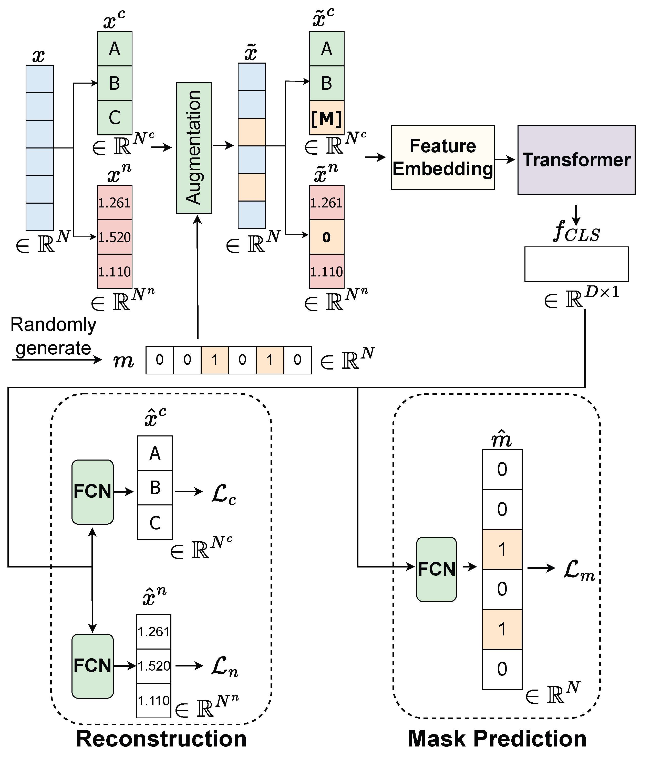
Our approach to data augmentation involves a technique called random feature discarding. This method systematically simulates missing data patterns to help the model learn robust representations even when features are absent. For a given data sample , we randomly produce a mask vector , where the dimension matches that of and the value 1 indicates the features that will be discarded. The process is describe in Figure 5.
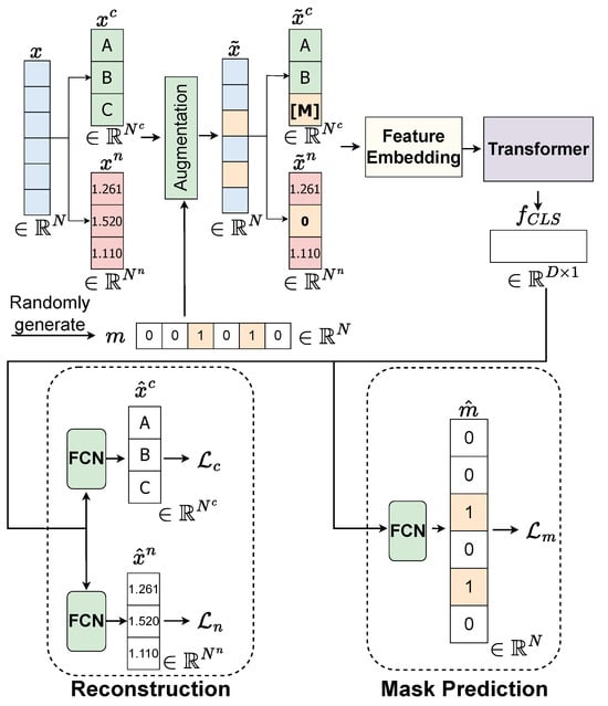
Figure 5.
Details of pretext task in our proposed SSL. Features are randomly discarded. Missing in the categorical feature will be treated as a distinct category [M]. Numerical features will be rescaled to fit within the range , and missing values are represented as 0. is feature representation [CLS] token extracted from feature map . is a predicted corrupted mask. represents the reconstructed categorical features. represents the reconstructed numerical features.
When dealing with numerical data, we rescale them to fit within the range and represent missing values as 0. This normalization ensures consistent handling across different numerical scales. In the case of categorical data, we treat missing values as a distinct category [M], which allows the model to explicitly recognize and learn patterns associated with missing categorical information.
By employing this method, we are able to generate a considerable amount of data from the original complete dataset for our pre-training objective without necessitating labeled information. This augmentation strategy effectively expands the training distribution, enabling the model to generalize better to various missing data scenarios encountered during inference.
3.3.2. Pre-Training
In the pretext task, we aim to pre-train a feature extraction component corresponding to the two models of Feature Embedding and Transformer. This pre-training module is designed to provide a pre-trained Feature Embedding model and pre-trained Transformer model, which are then transferred to the downstream task of survival prediction. To ensure both Feature Embedding and Transformer are robust against missing values, the proposed pre-training takes a complete feature as its input and outputs the feature , which is capable of being robust against missing values. To achieve this goal, we initiate the process by introducing an augmentation technique, as discussed in Section 3.3.1, to the original complete dataset x. This augmentation process generates synthetic data with missing values, denoted as . This augmented dataset includes categorical features , numerical features , and a corresponding missing mask m. Subsequently, we employ the Feature Embedding and Transformer components to extract feature representations from and , resulting in the feature representation for the instance . Within this pre-training module, both the Feature Embedding and Transformer models are trained on two pretext tasks: mask prediction and feature reconstruction. For each of these pretext tasks, we apply a Fully Connected Layer (FCN) to the feature .
In the mask prediction task, we denote as the predicted mask. The loss between the actual missing mask m and the predicted missing mask is computed using Binary Cross-Entropy (BCE) as follows: .
In the feature reconstruction task, we expect both the Feature Embedding and Transformer models to be robust in handling missing values in the corrupted categorical vector, meaning they should be capable of reconstructing given . The categorical reconstruction loss is defined as , where MBCE stands for Multi-Label Binary Cross-Entropy Loss. Additionally, by applying the Feature Embedding and Transformer models to the corrupted numerical vector , we aim to reconstruct the vector . Hence, the numerical reconstruction loss is defined as , where represents the reconstructed numerical vector.
Consequently, the pre-training procedure is trained using the following loss, which combines the mask prediction loss , categorical reconstruction loss , and numerical reconstruction loss .
where is a hyperparameter discussed in Appendix C, Table A5.
4. Experiments
4.1. Datasets
We evaluate the performance of our model as well as the baseline methods on datasets that include missing values. Specifically, we employ the METABRIC (https://www.cbioportal.org/study/summary?id=brca_metabric (accessed on 17 December 2023)) dataset [31], which consists of 1904 patients and encompasses 30 clinical attributes and 4 genetic attributes. Additionally, we make use of the SUPPORT (https://www.vumc.org/biostatistics/vanderbilt-department-biostatistics (accessed on 17 December 2023)) dataset [32], which comprises 9105 patients and includes 24 clinical features. We also compare our model’s performance with others on a complete dataset. Specifically, we choose another widely-used dataset, FLCHAIN [30], which includes an assay of serum free light chain for 6524 subjects, with 8 covariates. We obtain the dataset from the pycox library (https://github.com/havakv/pycox (accessed on 17 December 2023)). Our model is trained on 5-fold cross-validation, thus, each dataset is divided into 64/16/20 for training/validation/testing. Comprehensive details regarding the percentage of missing values and the maximum number of missing features are available in Table 2. Further information on the feature selection process can be found in the Appendix B.
Table 2.
Datasets summarization. “No. F” is number of features. “Max.No.M.F.” is maximum number of missing features in dataset. “M.R” is missing ratio in dataset.
4.2. Evaluation Metrics
In the realm of survival analysis, the concordance index (C-index) [59] and Brier score [60] are important metrics to evaluate the performance of the survival prediction model.
The C-index [59] measures the proportion of pairs of patients for which the predicted survival time agrees with the actual survival time. Specifically, it considers all pairs of patients in which at least one patient has died. For each pair, if the predicted survival time is larger for the patient who lived longer, the prediction is considered consistent with the outcome. The C-index can handle right-censored patients and provides an overall measure of the model’s predictive accuracy, ranging from 0 to 1, with larger values indicating better accuracy.
The Brier score [60] considers both discrimination and calibration. It is decomposed into two primary components: reliability and resolution. Reliability measures the closeness of predicted probabilities to the true probabilities, while resolution measures how much the conditional probabilities differ from the predictive average. The Brier score is a scalar value ranging from 0 to 1, with smaller values indicating superior prediction performance.
However, Harrell’s C-index [59], while widely adopted as the standard measure in survival analysis, has a fundamental limitation: it assumes proportional hazards, where a predictor’s effect on survival remains constant over time. This assumption often fails in clinical settings where treatment effects or risk factors may have varying impacts during different phases of disease progression. The time-dependent C-index [61] that we employ addresses this limitation by evaluating predictive accuracy at specific timepoints rather than assuming uniform effects throughout the follow-up period. This approach is particularly valuable for our study, where the impact of missing data on prediction accuracy may vary across different time horizons. We use C-index to indicate a time-dependent concordance index for now. We benchmark the proposed SSL-SurvFormer with two kinds evaluation based on the C-index and Brier score as follows:
Overall evaluation: The overall metrics include Integrated C-index (IC-index), Integrated Brier Score (IBS), and Integrated Negative Binomial Log-likelihood (INBLL) [62] at all available times of each dataset. The IC-index and IBS provide an overall calculation of the model performance on the C-index and Brier score at all available times, respectively. INBLL provides the measurement of both discrimination and calibration of the estimates of a method under every timepoint. A higher IC-index aand a lower IBS and INBLL are better. We employ integrated metrics (IC-index, IBS, and INBLL) to evaluate performance across the entire time spectrum rather than at isolated timepoints. This provides a more comprehensive evaluation of model performance with missing data, capturing both immediate and long-term predictive accuracy. Integrated metrics are especially appropriate in our context because the effects of missing values may manifest differently across the survival curve, and a comprehensive assessment over all available timepoints yields a more reliable comparison between methods than evaluations at arbitrary timepoints. Those metrics are used to evaluate continuous-time methods.
Quantile evaluation: The quantile metrics include the C-index [61] and Brier score [60] at the dataset-specific 0.25, 0.5, and 0.75 quantiles of the uncensored population event times. Those metrics are used to evaluate discrete-time methods.
The mathematical formulas of the metrics are reported in the Appendix A.
4.3. Implementation Details
Based on two kinds of evaluation metrics, we have implemented the model in two scenarios as follows:
Overall evaluation: We followed [13,15] and evaluated our SSL-SurvFormer models over the entire observed duration. Specifically, we used the models to inference at 1000 timepoints that are evenly distributed across the timescale. Overall metrics are computed on all these timepoints. In this evaluation, we are comparing our model with three other existing effective models: the Cox Proportional Hazard (CoxPH) model [7], DeepSurv [15], and SuMo-Net [13]. The CoxPH [7] model estimates survival outcomes by creating a linear combination of covariates as expressed by the formula: . DeepSurv [15], on the other hand, is an extension of CoxPH that employs a neural network instead of a linear model for its calculations. Meanwhile, SuMo-Net [13] utilizes an MLP network with a positive constraint on the model’s weights to estimate the cumulative distribution function , which is described in Section 3.2.3. This approach closely resembles our own method. To compare our SSL-SurvFormer with the existing methods for handling missing data, we used two common approaches as baselines: mean and mode (MM) imputation and KNN imputation, as described in Section 2. Specifically, when dealing with categorical data, we applied mode imputation, which involved filling in missing values with the most frequently occurring value in the dataset. For numerical data, we opted for mean imputation, replacing the missing values with the average value. The implementations of MM and KNN followed those in [63].
Quantile evaluation: We followed [14,16] and set the last layer to a vector in five-dimensional space, which reflects the output at the 0, 0.25, 0.5, 0.75, and 1 quantiles. In this case, we compare the performance of our proposed methods with two well-known discrete-time models, i.e., DeepHit [14] and SurvTRACE [16], which are directly optimized on these discrete points. The performance is reported at 0.25, 0.5, and 0.75. As with the overall evaluation, we applied both MM and KNN imputation techniques to address missing data.
Regarding hyperparameters, we have followed the widely used settings [13,28,29] and conducted hyperparameter search spaces to find the optimal configuration. The details of search spaces are included in the Appendix C. We implemented our method in Pytorch. To conduct a fair comparison, we used the AdamW optimizer [64] with early stopping set at 10 iterations for our methods and other existing work. All of our experiments were trained, evaluated on a GPU Tesla T4 16 GB, and conducted under the same conditions in terms of package versions. All the requirements of software libraries and frameworks will be made publicly available along with the code upon publication of the paper.
4.4. Performance Comparison
Our primary objective is to compare our method with other deep learning and Transformer-based approaches that have demonstrated superiority over conventional techniques (such as Cox regression [7] and Kaplan–Meier estimation [6]) in previous studies. We classify survival prediction methods into two groups based on discrete time and continuous time in Table 1. Consequently, we compare our proposed SSL-SurvFormer with the existing SOTA in each group as follows:
Overall Comparison with continuous-time methods: Table 3 reports the overall performance comparison on two missing-value datasets between our proposed SSL-SurvFormer and continuous-time methods: Cox Regression [7], DeepSurv [15], and Sumo-Net [13]. We conducted this comparison using both imputation approaches, namely mean and mode (MM) imputation and KNN imputation, for the baselines, as mentioned in Section 4.3. The findings indicate that the KNN imputation method exhibits superior performance when compared to the MM approach. Nevertheless, it is evident from the results that our SSL-SurvFormer model outperforms the other models, regardless of the imputation method used, highlighting its effectiveness in survival analysis, particularly when confronted with datasets containing missing data.
Table 3.
Overall performance comparison on two missing datasets: METABRIC (MET.) [31] and SUPPORT (SUP.) [32] between our proposed SSL-SurvFormer and the continuous-time methods DeepSurv [15] and Sumo-Net [13]. Results are reported as mean (standard deviation) over the 5-fold cross validation. On each dataset, the best is shown in bold. MM and KNN stand for mean and mode and K-nearest neighbor, respectively.
In particular, our SSL-SurvFormer demonstrates a noteworthy advantage when compared to other baseline models. When we compare our model to SuMo-Net [13] and DeepSurv [15], utilizing both KNN imputation and MM imputation on the METABRIC [31] dataset, our model consistently achieves a higher IC-index, with gaps of 0.012, 0.015, 0.016, and 0.018, respectively. Furthermore, our model significantly improves the INBLL [62], with gaps of 0.012, 0.019, 0.020, and 0.027 in comparison to SuMo-Net [13] and DeepSurv [15] using these two imputation methods.
Similarly, when comparing our model to SuMo-Net [13] and DeepSurv [15], utilizing both MM imputation and KNN imputation on the SUPPORT [32] dataset, our SSL-SurvFormer demonstrates a higher IC-index, with gaps of 0.029, 0.035, 0.040, and 0.040, respectively. Additionally, our model improves the INBLL by 0.012, 0.017, 0.031, and 0.035 when compared to SuMo-Net [13] and DeepSurv [15] using these two imputation methods.
In other comparisons, our model consistently surpasses the other baseline models with a competitive margin. This serves as strong evidence of its superiority in addressing survival analysis problems.
Quantile Comparison with discrete-time approaches: Table 4 reports the quantile performance comparison at 0.25, 0.5, and 0.75 between our SSL-SurvFormer and existing SOTA discrete-time approaches, namely DeepHit [14] and SurvTrace [16]. It is worth noting that the KNN imputation method consistently outperforms the MM approach, aligning with the findings in the overall comparison. However, what remains consistent across all scenarios is that our SSL-SurvFormer model consistently outperforms the two baseline models—DeepHit [14] and SurvTrace—across all quantiles and with both imputation strategies. As an example, when we compare our proposed model to the second-best performer, SurvTRACE [16] with KNN imputation, on the METABRIC [31] dataset, our model demonstrates a significant performance advantage in terms of the C-index across three quantiles. The performance gaps are notable, measuring 0.009, 0.008, and 0.007, respectively. Likewise, when we evaluate our model against the second-best performer, SurvTRACE [16] with KNN imputation, on the SUPPORT [32] dataset, our model outperforms it with substantial performance differences, measuring 0.012, 0.017, and 0.012 across three quantiles. Furthermore, SSL-Survformer outperforms SurvTRACE [16] with KNN imputation by achieving lower Brier scores across three quantiles, with differences of 0.004, 0.011, and 0.007 on the METABRIC [31] dataset and 0.006, 0.016, and 0.009 on the SUPPORT [32] dataset.
Table 4.
Quantile performance comparison between SSL-SurvFormer and discrete-time methods on two missing datasets. Results are reported as mean (standard deviation) over the 5-fold cross validation. On each dataset, the best is shown in bold. CI and BS stand for C-index and Brier score, respectively. MM and KNN stand for mean and mode and K-nearest neighbor, respectively.
Comparision on Complete Data Table 5 and Table 6 display our performance relative to other baseline models on the fully complete FLCHAIN [30] dataset. The findings demonstrate that SSL-SurvFormer excels not only on datasets with missing features but also surpasses other methods on datasets without any missing data. Specifically, our model outperforms the second-best SuMo-Net [13] across all overall metrics, with a noticeable gap of 0.007 on the IC-index, 0.01 on INBLL, and 0.004 on IBS. Moreover, when it comes to quantile metrics, our model achieves competitive results when compared to SurvTRACE [16] and surpasses DeepHit [14] with differences of 0.002, 0.007, and 0.004 on three quantiles, respectively, for the C-Index. Additionally, our model outperforms DeepHit [14] with differences of 0.024, 0.037, and 0.085 on three quantiles for the Brier score.
Table 5.
Overall performance comparison on the no-missing value dataset FLCHAIN [30] between our proposed SSL-SurvFormer and continuous-time methods: Cox Regression [7], DeepSurv [15], and Sumo-Net [13]. Results are reported as mean (standard deviation) over the 5-fold cross validation. The best is shown in bold.
Table 6.
Quantile performance comparison between SurvFormer, SSL-SurvFormer, and discrete-time methods on the no-missing value dataset FLCHAIN [30]. Results are reported as mean (standard deviation) over the 5-fold cross validation. The best is shown in bold. CI and BS stand for C-index and Brier score, respectively.
4.5. Results Analysis
To evaluate the effectiveness of our proposed SSL-SurvFormer, we compare its performance on different kind of data, namely uncensored data and censored data. From Section 4.4, we can see that SSL-SurvFormer surpasses other methods on datasets that contain missing values; therefore, we continue investigating more deeply how our model and the others perform when the missing ratio gradually increases.
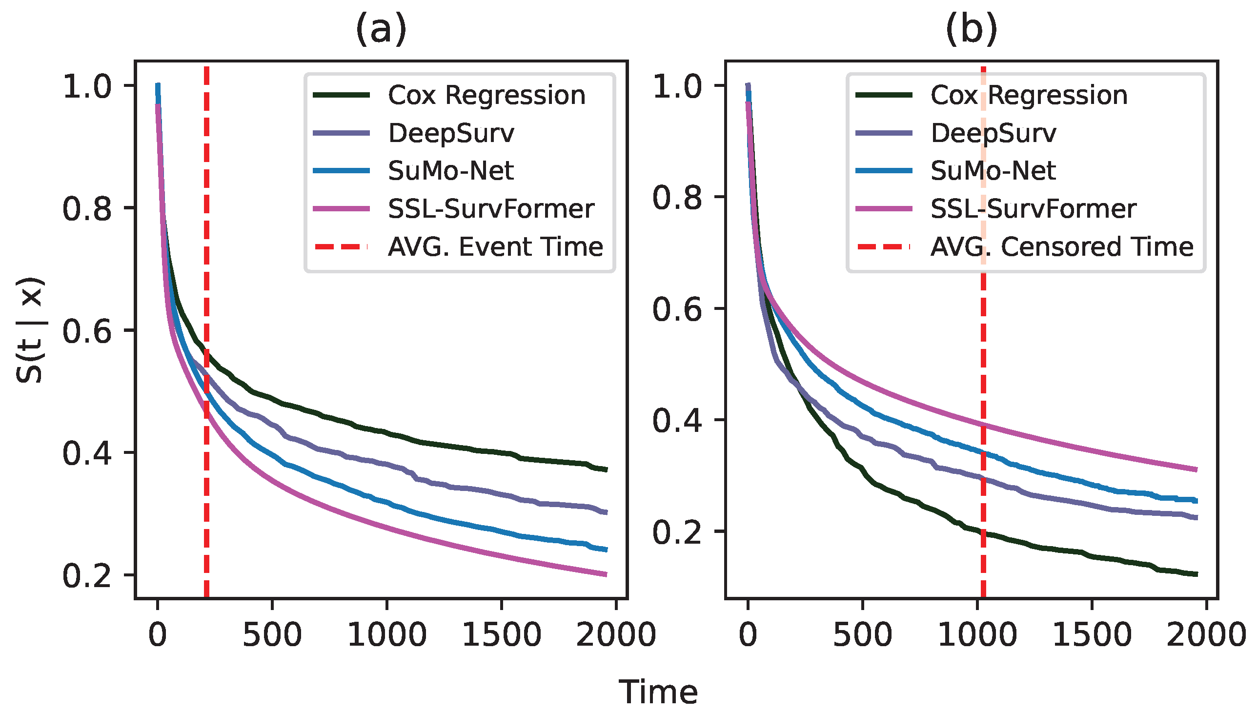
Comparison on uncensored data and censored data. To conduct this experiment, we use SUPPORT [32] data as an example. Based on whether or not an event occurs, we separate 1821 samples in the testset into two subsets of 1242 uncensored samples (event occurs) and 579 censored samples (event does not occur). Figure 6 shows the comparison of average survival curves between SSL-SurvFormer and other continuous-time methods on both uncensored data (a) and censored data (b). The figure shows that when an event happens, our method can better detect the occurrence of the event than the others, i.e., our predicted survival probability drops at the time of the event and maintains low values. In contrast, DeepSurv [15] and SuMo-Net [13] have limitations in identifying the event signal and their survival probabilities are still high at the event time. On the censored data, i.e., when an event does not happen, SSL-SurvFormer succeeds in maintaining a high survival probability before the censored timepoint.
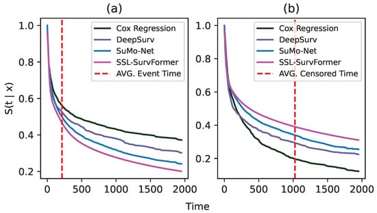
Figure 6.
Average predicted survival function on two subsets of uncensored data (a) and censored data (b). These subsets are extracted from the testset of the SUPPORT [32] dataset. In these figures, the x-axis denotes duration timepoints and the y-axis shows the probability . Dashed lines (- - -) indicate the average timepoint where the event/censoring happens.
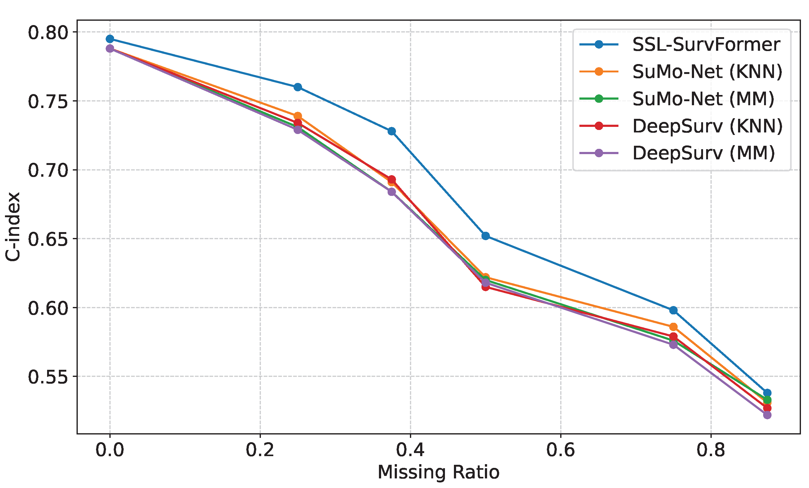
Comparison on different missing value ratios. We evaluated our model’s performance using the FLCHAIN [30] dataset, which contains eight features per sample. We systematically removed zero, two, three, four, five, or six random features, corresponding to missing value ratios of 0, 0.25, 0.375, 0.5, 0.625, and 0.75, respectively. Figure 7 demonstrates that SSL-SurvFormer consistently outperforms baseline models across all missing value ratios, with particularly significant performance gaps at ratios of 0.25, 0.375, and 0.5. These results indicate the robustness of SSL-SurvFormer in handling missing data scenarios.
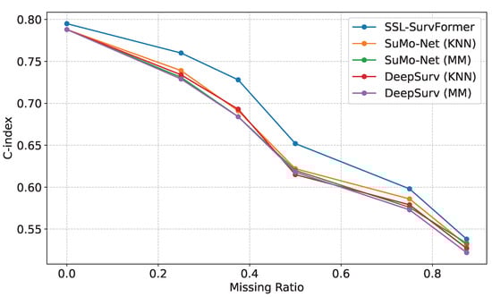
Figure 7.
Performance comparison of the models on the FLCHAIN [30] dataset with varying proportions of missing values. SSL-SurvFormer demonstrates superior C-index scores, particularly at 0.25, 0.375, and 0.5 missing data ratios.
4.6. Ablation Study
We analyze the contribution of SSL in SSL-SurvFormer by comparing the SSL-SurvFormer with SurvFormer by removing SSL pre-training and investigating SSL pre-training by considering the impact of each loss term defined in Equation (7).
Efficiency of SSL in SSL-SurvFormer. We analyze the effectiveness of our proposed SSL pre-training in SSL-SurvFormer by first removing the SSL from SSL-SurvFormer (i.e., it becomes SurvFormer) and then investigating the contribution of individual components in SSL. Table 7 compares the performance of SurvFormer and SSL-SurvFormer on the FLCHAIN [30] dataset, which is a dataset with no missing values. Moreover, the SSL pre-train in SSL-SurvFormer is trained by , as defined in Equation (7). In particular, it is trained on augmented data through mask prediction and reconstruction via . We demonstrate the impact of each loss term in Table 7 and Table 8. We also compare the performance of model with each loss on the dataset with missing values, i.e., the SUPPORT [32] dataset, where we pre-train our model with limited complete data (with augmentation technique) and finetune it with all the available data (missing values included). This ablation study indicates that while pre-training with either corrupted mask prediction or reconstruction can improve performance, the combination of both losses in yields the best results. On the FLCHAIN [30] dataset, which is entirely complete, SSL leads to a performance improvement of 0.002, 0.007, and 0.003 in terms of the IC-index, IBS, and INBLL, respectively. Furthermore, when dealing with the missing data in the SUPPORT [32] dataset, pre-training with the combined losses in results in a performance boost of 0.02, 0.006, and 0.009 for the IC-index, IBS, and INBLL, respectively.
Table 7.
The impact of each component in SSL pre-training on the FLCHAIN [30] dataset (fully complete dataset). The baseline is our SurvFormer model without pre-training with SSL.
Table 8.
The impact of each component in SSL pre-training on the SUPPORT [32] dataset (missing dataset). The baseline is our SurvFormer model without pre-training with SSL. When remove SSL, we use KNN imputation for missing values.
5. Conclusions
This paper introduces SSL-SurvFormer, a novel continuously monotonic Transformer-based model designed for robust survival prediction. Our model incorporates Transformer architecture and a monotonically positive neural network, enabling efficient survival prediction without the need to discretize time intervals. Additionally, we leverage self-supervised learning (SSL) techniques, coupled with our proposed data augmentation, to effectively handle missing values in the data. Our extensive experiments and comprehensive ablation study, conducted on three diverse datasets (METABRIC [31], SUPPORT [32], and FLCHAIN [30]) encompassing scenarios with and without missing features, demonstrate the superior performance of SSL-SurvFormer. It outperforms current state-of-the-art methods, both discrete-time and continuous-time methods, in terms of quantile metrics and overall performance metrics.
In our future research endeavors, we intend to explore various self- and semi-supervised learning techniques. This exploration aims to enhance feature learning, potentially further improving our model’s robustness and performance. Additionally, we plan to investigate the development of loss functions that maintain monotonic constraints to expand its applicability to a broader range of survival prediction tasks.
Author Contributions
Conceptualization, Q.-H.L. and N.L.; methodology, Q.-H.L. and N.L.; experiments, Q.-H.L.; writing—original draft preparation, Q.-H.L.; writing—review and editing, B.P., D.A., G.D. and N.L.; visualization, Q.-H.L.; supervision, N.L. All authors discussed the results and contributed to the final manuscript. All authors have read and agreed to the published version of the manuscript.
Funding
Quang-Hung Le is supported by FPT Software Company Limited. Donald Adjeroh, Gianfranco Doretto and Ngan Le are supported by National Science Foundation (NSF) under Award NSF 2223793 EFRI BRAID.
Institutional Review Board Statement
Not applicable.
Informed Consent Statement
Not applicable.
Data Availability Statement
The study utilized METABRIC, a dataset that is publicly available at https://www.cbioportal.org/study/summary?id=brca_metabric (accessed on 17 December 2023); SUPPORT, available at https://www.vumc.org/biostatistics/vanderbilt-department-biostatistics (accessed on 17 December 2023)) and FLCHAIN, available through the pycox library https://github.com/havakv/pycox (accessed on 17 December 2023)).
Conflicts of Interest
The authors declare no conflicts of interest.
Appendix A. Evaluation Metric Details
Appendix A.1. Quantile Metrics
Concordance Index. The concordance index or C-index is a generalization of the area under the ROC curve (AUC) that can take into account right-censored data. It captures the discrimination power of the model: this is the model’s ability to correctly provide a reliable ranking of the survival times based on the individual risk scores. The quantile C-index assesses the model performance at the specific time t. Similar to the AUC, corresponds to the best model prediction and represents a random prediction.
For every pair of instances and (with ) and a given timepoint t, the C-index can be computed with the following formula:
- 1.
- is the time event really occurred or censored.
- 2.
- , the risk score of instance i at time t.
- 3.
- if else 0.
- 4.
- if event occurred, else 0.
Brier Score. The Brier score is used to evaluate the accuracy of a predicted survival function at a given time t; it represents the average squared distances between the observed survival status and the predicted survival probability and is always a number between 0 and 1, with 0 being the best possible value. A lower Brier score indicates a more accurate predicted survival function.
Given a dataset of Z samples, is the format of a data point, and the predicted survival function is . Let be the estimator of the conditional survival function of the censoring times calculated using the Kaplan–Meier method, where C is the censoring time, the Brier score can be calculated such that:
Appendix A.2. Overall Metrics
Integrated Time-dependent Concordance Index. Similar to the C-index, but the IC-index represents the discriminative performance of the model at all the available timepoints.
For every pair of instances and (with ), we look at their risk scores and times-to-event. Integrated C-index can be computed with the following formula:
with:
- 1.
- is the time event really occurred or censored.
- 2.
- , the risk score of instance i at the time .
- 3.
- if else 0.
- 4.
- if event occurred, else 0.
Integrated Brier Score. Similar to the Brier score, but the IBS represents the discriminative performance of the model at all the available timepoints. Following Equation (A2), the Integrated Brier Score (IBS) can be calculated as:
In terms of benchmarks, a useful model will have a Brier score below . Indeed, it is easy to see that if , then .
Negative Binomial LogLikelihood (NBLL).
The mean binomial log-likelihood is a commonly used metric in binary classification that measures both the discrimination and calibration of the estimates of a method. Following on from the above IBS discussion definition, the authors of [22] define the negative log-likelihood of the variable and integrate this over time to obtain the Integrated Negative Binomial Log-Likelihood (INBLL), a metric for which smaller values indicate better classification performance.
The -scaled) negative log-likelihood for the random variable at time t is:
Applying the same censoring weighting as previously provides
To obtain the INBLL metric, this can be integrated in the IBS:
Appendix B. Datasets
In Section 4.1, we mentioned two datasets that include missing values: METABRIC [31] and SUPPORT. For the METABRIC [31] dataset, we chose 4 genetic features (MKI67, EGFR, PGR, and ERBB2) and 29 clinical features (Age at Diagnosis, Type of Breast Surgery, Cancer Type Detailed, Cellularity, Chemotherapy, Pam50 + Claudin-low subtype, Cohort, ER status measured by IHC, ER Status, Neoplasm Histologic Grade, HER2 status measured by SNP6, HER2 Status, Tumor Other Histologic Subtype, Hormone Therapy, Inferred Menopausal State, Integrative Cluster, Primary Tumor Laterality, Lymph nodes examined positive, Mutation Count, Nottingham prognostic index, Oncotree Code, PR Status, Radio Therapy, Relapse Free Status (Months), Relapse Free Status, 3-Gene classifier subtype, TMB (nonsynonymous), Tumor Size, and Tumor Stage). For the SUPPORT [32] dataset, we chose 24 patient covariates, including age, gender, race, income, co-morbidity information, heart rate, mean blood pressure, temperature, respiratory rate, serum creatinine, serum albumin, serum bilirubin, serum sodium, PaO2/FiO2 ratio, Urine output, BUN, glucose, white blood count, cancer indication, disease group, disease class, activities of daily living, and imputed activities of daily living calibrated to surrogate. For the FLCHAIN [30] dataset, we follow the feature selection and feature pre-processing of [62].
Appendix C. Hyperparameters Search Spaces
In Section 4.3 of the main paper, we have followed the widely used implementation [13,16,29] and conducted hyperparameter search spaces to find the optimal configuration. Below, we first recap searching space by existing SOTA approaches, i.e., DeepHit [14], DeepSurv [15], SuMo-Net [13], and SurvTRACE [16]. Then, we detail hyperparameter search spaces in our proposed sSL-SurveFormer.
Table A1.
Hyperparameters of MLP-based models: DeepHit and DeepSurv. Loss and Loss are the only hyperparameters in DeepHit.
Table A1.
Hyperparameters of MLP-based models: DeepHit and DeepSurv. Loss and Loss are the only hyperparameters in DeepHit.
| Hyperparameter | Values |
|---|---|
| Layers | |
| Nodes per layer | |
| Dropout | |
| Weigh decay | |
| Learning rate | |
| Batch size | |
| Loss (DeepHit) | |
| Loss (DeepHit) |
Table A2.
Hyperparameters of SuMo-Net.
Table A2.
Hyperparameters of SuMo-Net.
| Hyperparameter | Values |
|---|---|
| Layers | |
| Layers Positive | |
| Nodes per layer | |
| Nodes per positive layer | |
| Dropout | |
| Weigh decay | |
| Learning rate | |
| Batch size |
In Table A4, we provide the detailed hyperparameter search space of our proposed SurvFormer. The feature embedding size (D) is the dimensional space of feature embedding, which is generated from one patient’s feature attribute. This is illustrated in Figure 2. The number of attention heads is the hyperparameter corresponding to the Multi-head Self-Attention layer (Figure 3). The number of positive layers, in which each node is connected by red dash line (Figure 4), and the number of nodes per positive layer are hyperparameters corresponding to the monotonically positive component of SurvFormer. The hyperparameters and correspond to our losses. Our loss function is combination of a log-likelihood loss in Equation (4) and an order loss in Equation (5). Our final loss function can be described as in Equation (6).
Table A3.
Hyperparameters of SurvTRACE.
Table A3.
Hyperparameters of SurvTRACE.
| Hyperparameter | Values |
|---|---|
| Feature embedding size | |
| Attention heads | |
| Learning rate | |
| Weigh decay | |
| Batch size |
Table A4.
Hyperparameters of our proposed SurvFormer. Other hyperparameters of Transformer are used similarly to the default configuration in [12].
Table A4.
Hyperparameters of our proposed SurvFormer. Other hyperparameters of Transformer are used similarly to the default configuration in [12].
| Hyperparameter | Values |
|---|---|
| Feature embedding size (D) | |
| No. attention heads | |
| No. layers Positive | |
| No. nodes per positive layer | |
| Learning rate | |
| Weigh decay | |
| Batch size | |
| Loss | |
| Loss |
Table A5.
Hyperparameters for pre-training SSL.
Table A5.
Hyperparameters for pre-training SSL.
| Hyperparameter | Values |
|---|---|
| Corrupt ratio | |
| Learning rate | |
| Weigh decay | |
| Batch size | |
| Loss |
References
- Ziehm, M.; Thornton, J.M. Unlocking the potential of survival data for model organisms through a new database and online analysis platform: SurvCurv. Aging Cell 2013, 12, 910–916. [Google Scholar] [CrossRef] [PubMed]
- Susto, G.A.; Schirru, A.; Pampuri, S.; McLoone, S.; Beghi, A. Machine Learning for Predictive Maintenance: A Multiple Classifier Approach. IEEE Tran. Ind. Inf. 2015, 11, 812–820. [Google Scholar] [CrossRef]
- Laurie, J.A.; Moertel, C.G.; Fleming, T.R.; Wieand, H.S.; Leigh, J.E.; Rubin, J.; McCormack, G.W.; Gerstner, J.B.; Krook, J.E.; Malliard, J. Surgical adjuvant therapy of large-bowel carcinoma: An evaluation of levamisole and the combination of levamisole and fluorouracil. The North Central Cancer Treatment Group and the Mayo Clinic. J. Clin. Oncol. 1989, 7, 1447–1456. [Google Scholar] [CrossRef] [PubMed]
- Dirick, L.; Claeskens, G.; Baesens, B. Time to default in credit scoring using survival analysis: A benchmark study. J. Oper. Res. Soc. 2017, 68, 652–665. [Google Scholar] [CrossRef]
- Van den Poel, D.; Larivière, B. Customer attrition analysis for financial services using proportional hazard models. Eur. J. Oper. Res. 2004, 157, 196–217. [Google Scholar] [CrossRef]
- Kaplan, E.L.; Meier, P. Nonparametric Estimation from Incomplete Observations. J. Am. Stat. Assoc. 1958, 53, 457–481. [Google Scholar] [CrossRef]
- Cox, D.R. Regression Models and Life-Tables. J. R. Stat. Soc. Ser. B (Methodol.) 1972, 34, 187–220. [Google Scholar] [CrossRef]
- Kalbfleisch, J.D.; Prentice, R.L. The Statistical Analysis of Failure Time Data; John Wiley & Sons: Hoboken, NJ, USA, 2011. [Google Scholar]
- Pölsterl, S.; Navab, N.; Katouzian, A. Fast training of support vector machines for survival analysis. In Proceedings of the Joint European Conference on Machine Learning and Knowledge Discovery in Databases, Porto, Portugal, 7–11 September 2015; pp. 243–259. [Google Scholar]
- Van Belle, V.; Pelckmans, K.; Suykens, J.A.; Van Huffel, S. Support vector methods for survival analysis: A comparison between ranking and regression approaches. Artif. Intell. Med. 2011, 53, 107–118. [Google Scholar] [CrossRef]
- Ishwaran, H.; Kogalur, U.B.; Blackstone, E.H.; Lauer, M.S. Random survival forests. Ann. Appl. Stat. 2008, 2, 841–860. [Google Scholar] [CrossRef]
- Wang, X.; Pakbin, A.; Mortazavi, B.; Zhao, H.; Lee, D. BoXHED: Boosted exact Hazard estimator with dynamic covariates. In Proceedings of the ICML, Virtual, 13–18 July 2020; pp. 9973–9982. [Google Scholar]
- Rindt, D.; Hu, R.; Steinsaltz, D.; Sejdinovic, D. Survival regression with proper scoring rules and monotonic neural networks. In Proceedings of the International Conference on Artificial Intelligence and Statistics, Virtual, 28–30 March 2022; pp. 1190–1205. [Google Scholar]
- Lee, C.; Zame, W.; Yoon, J.; Van Der Schaar, M. Deephit: A deep learning approach to survival analysis with competing risks. In Proceedings of the AAAI Conference on Artificial Intelligence, New Orleans, LA, USA, 2–7 February 2018; Volume 32. [Google Scholar]
- Katzman, J.L.; Shaham, U.; Cloninger, A.; Bates, J.; Jiang, T.; Kluger, Y. DeepSurv: Personalized treatment recommender system using a Cox proportional hazards deep neural network. BMC Med. Res. Methodol. 2018, 18, 24. [Google Scholar] [CrossRef]
- Wang, Z.; Sun, J. Survtrace: Transformers for survival analysis with competing events. In Proceedings of the ACM International Conference on Bioinformatics, Computational Biology and Health Informatics, Northbrook, IL, USA, 7–10 August 2022; pp. 1–9. [Google Scholar]
- Hu, S.; Fridgeirsson, E.; van Wingen, G.; Welling, M. Transformer-based deep survival analysis. In Proceedings of the Survival Prediction-Algorithms, Challenges and Applications, Palo Alto, CA, USA, 22–24 March 2021; pp. 132–148. [Google Scholar]
- Devlin, J.; Chang, M.W.; Lee, K.; Toutanova, K. Bert: Pre-training of deep bidirectional transformers for language understanding. arXiv 2018, arXiv:1810.04805. [Google Scholar]
- Brown, T.; Mann, B.; Ryder, N.; Subbiah, M.; Kaplan, J.D.; Dhariwal, P.; Neelakantan, A.; Shyam, P.; Sastry, G.; Askell, A.; et al. Language models are few-shot learners. NIPS 2020, 33, 1877–1901. [Google Scholar]
- Truong, T.D.; Duong, C.N.; Pham, H.A.; Raj, B.; Le, N.; Luu, K. The right to talk: An audio-visual transformer approach. In Proceedings of the IEEE/CVF International Conference on Computer Vision, Montreal, BC, Canada, 11–17 October 2021; pp. 1105–1114. [Google Scholar]
- Karita, S.; Chen, N.; Hayashi, T.; Hori, T.; Inaguma, H.; Jiang, Z.; Someki, M.; Soplin, N.E.Y.; Yamamoto, R.; Wang, X.; et al. A comparative study on transformer vs rnn in speech applications. In Proceedings of the 2019 IEEE Automatic Speech Recognition and Understanding Workshop (ASRU), Singapore, 14–18 December 2019. [Google Scholar]
- Dong, L.; Xu, S.; Xu, B. Speech-transformer: A no-recurrence sequence-to-sequence model for speech recognition. In Proceedings of the 2018 IEEE International Conference on Acoustics, Speech and Signal Processing (ICASSP), Calgary, AB, Canada, 15–20 April 2018; pp. 5884–5888. [Google Scholar]
- Dosovitskiy, A.; Beyer, L.; Kolesnikov, A.; Weissenborn, D.; Zhai, X.; Unterthiner, T.; Dehghani, M.; Minderer, M.; Heigold, G.; Gelly, S.; et al. An image is worth 16x16 words: Transformers for image recognition at scale. arXiv 2020, arXiv:2010.11929. [Google Scholar]
- Liu, Z.; Lin, Y.; Cao, Y.; Hu, H.; Wei, Y.; Zhang, Z.; Lin, S.; Guo, B. Swin transformer: Hierarchical vision transformer using shifted windows. In Proceedings of the IEEE/CVF Conference on Computer Vision and Pattern Recognition (CVPR), Nashville, TN, USA, 20–25 June 2021. [Google Scholar]
- Tran, M.; Vo, K.; Yamazaki, K.; Fernandes, A.; Kidd, M.; Le, N. AISFormer: Amodal Instance Segmentation with Transformer. arXiv 2022, arXiv:2210.06323. [Google Scholar]
- Yamazaki, K.; Vo, K.; Truong, Q.S.; Raj, B.; Le, N. VLTinT: Visual-linguistic transformer-in-transformer for coherent video paragraph captioning. In Proceedings of the AAAI Conference on Artificial Intelligence, Washington, DC, USA, 7–14 February 2023; Volume 37, pp. 3081–3090. [Google Scholar]
- Vo, K.; Truong, S.; Yamazaki, K.; Raj, B.; Tran, M.T.; Le, N. Aoe-net: Entities interactions modeling with adaptive attention mechanism for temporal action proposals generation. Int. J. Comput. Vis. 2023, 131, 302–323. [Google Scholar] [CrossRef]
- Huang, X.; Khetan, A.; Cvitkovic, M.; Karnin, Z. TabTransformer: Tabular Data Modeling Using Contextual Embeddings. arXiv 2020, arXiv:2012.06678. [Google Scholar]
- Gorishniy, Y.; Rubachev, I.; Khrulkov, V.; Babenko, A. Revisiting Deep Learning Models for Tabular Data. arXiv 2021, arXiv:2106.11959. [Google Scholar]
- Dispenzieri, A.; Katzmann, J.A.; Kyle, R.A.; Larson, D.R.; Therneau, T.M.; Colby, C.L.; Clark, R.J.; Mead, G.P.; Kumar, S.; Melton, L.J., III; et al. Use of nonclonal serum immunoglobulin free light chains to predict overall survival in the general population. Mayo Clin. Proc. 2012, 87, 517–523. [Google Scholar] [CrossRef]
- Curtis, C.; Shah, S.P.; Chin, S.F.; Turashvili, G.; Rueda, O.M.; Dunning, M.J.; Speed, D.; Lynch, A.G.; Samarajiwa, S.; Yuan, Y.; et al. The genomic and transcriptomic architecture of 2000 breast tumours reveals novel subgroups. Nature 2012, 486, 346–352. [Google Scholar] [CrossRef]
- Knaus, W.A.; Harrell, F.E.; Lynn, J.; Goldman, L.; Phillips, R.S.; Connors, A.F.; Dawson, N.V.; Fulkerson, W.J.; Califf, R.M.; Desbiens, N.; et al. The SUPPORT prognostic model: Objective estimates of survival for seriously ill hospitalized adults. Ann. Intern. Med. 1995, 122, 191–203. [Google Scholar] [CrossRef]
- Rumelhart, D.E.; Hinton, G.E.; Williams, R.J. Learning representations by back-propagating errors. Nature 1986, 323, 533–536. [Google Scholar] [CrossRef]
- Tang, W.; Ma, J.; Mei, Q.; Zhu, J. SODEN: A Scalable Continuous-Time Survival Model through Ordinary Differential Equation Networks. J. Mach. Learn. Res. 2022, 23, 1–29. [Google Scholar]
- Ausset, G.; Ciffreo, T.; Portier, F.; Clémençon, S.; Papin, T. Individual Survival Curves with Conditional Normalizing Flows. In Proceedings of the IEEE 8th International Conference on Data Science and Advanced Analytics (DSAA), Porto, Portugal, 6–9 October 2021; pp. 1–10. [Google Scholar]
- Danks, D.; Yau, C. Derivative-Based Neural Modelling of Cumulative Distribution Functions for Survival Analysis. In Proceedings of the International Conference on Artificial Intelligence and Statistics, Virtual, 28–30 March 2022; pp. 7240–7256. [Google Scholar]
- Dupont, E.; Doucet, A.; Teh, Y.W. Augmented neural odes. Adv. Neural Inf. Process. Syst. 2019, 32. [Google Scholar] [CrossRef]
- Massaroli, S.; Poli, M.; Park, J.; Yamashita, A.; Asama, H. Dissecting neural odes. Adv. Neural Inf. Process. Syst. 2020, 33, 3952–3963. [Google Scholar]
- Vaswani, A.; Shazeer, N.; Parmar, N.; Uszkoreit, J.; Jones, L.; Gomez, A.N.; Kaiser, Ł.; Polosukhin, I. Attention is all you need. NIPS 2017, 30. [Google Scholar] [CrossRef]
- Carion, N.; Massa, F.; Synnaeve, G.; Usunier, N.; Kirillov, A.; Zagoruyko, S. End-to-end object detection with transformers. In Proceedings of the Computer Vision—ECCV 2020: 16th European Conference, Glasgow, UK, 23–28 August 2020; Proceedings, Part I 16. Springer: Cham, Switherland, 2020; pp. 213–229. [Google Scholar]
- Liu, S.; Li, F.; Zhang, H.; Yang, X.; Qi, X.; Su, H.; Zhu, J.; Zhang, L. DAB-DETR: Dynamic anchor boxes are better queries for DETR. arXiv 2022, arXiv:2201.12329. [Google Scholar]
- Li, F.; Zhang, H.; Liu, S.; Guo, J.; Ni, L.M.; Zhang, L. Dn-detr: Accelerate detr training by introducing query denoising. In Proceedings of the IEEE/CVF Conference on Computer Vision and Pattern Recognition, New Orleans, LA, USA, 18–24 June 2022; pp. 13619–13627. [Google Scholar]
- Donders, A.R.T.; Van Der Heijden, G.J.; Stijnen, T.; Moons, K.G. A gentle introduction to imputation of missing values. J. Clin. Epidemiol. 2006, 59, 1087–1091. [Google Scholar] [CrossRef]
- Sinharay, S.; Stern, H.S.; Russell, D. The use of multiple imputation for the analysis of missing data. Psychol. Methods 2001, 6, 317. [Google Scholar] [CrossRef]
- Jerez, J.M.; Molina, I.; García-Laencina, P.J.; Alba, E.; Ribelles, N.; Martín, M.; Franco, L. Missing data imputation using statistical and machine learning methods in a real breast cancer problem. Artif. Intell. Med. 2010, 50, 105–115. [Google Scholar] [CrossRef]
- Yoon, J.; Jordon, J.; Schaar, M. Gain: Missing data imputation using generative adversarial nets. In Proceedings of the International Conference on Machine Learning, Stockholm, Sweden, 10–15 July 2018; pp. 5689–5698. [Google Scholar]
- McCoy, J.T.; Kroon, S.; Auret, L. Variational autoencoders for missing data imputation with application to a simulated milling circuit. IFAC-PapersOnLine 2018, 51, 141–146. [Google Scholar] [CrossRef]
- Wang, Q.; Li, B.; Xiao, T.; Zhu, J.; Li, C.; Wong, D.F.; Chao, L.S. Learning deep transformer models for machine translation. arXiv 2019, arXiv:1906.01787. [Google Scholar]
- Ba, J.L.; Kiros, J.R.; Hinton, G.E. Layer normalization. arXiv 2016, arXiv:1607.06450. [Google Scholar]
- Narang, S.; Chung, H.W.; Tay, Y.; Fedus, L.; Févry, T.; Matena, M.; Malkan, K.; Fiedel, N.; Shazeer, N.; Lan, Z.; et al. Do Transformer Modifications Transfer Across Implementations and Applications? In Proceedings of the 2021 Conference on Empirical Methods in Natural Language Processing, Virtual, 7–11 November 2021; pp. 5758–5773. [Google Scholar]
- Shazeer, N. Glu variants improve transformer. arXiv 2020, arXiv:2002.05202. [Google Scholar]
- Chilinski, P.; Silva, R. Neural likelihoods via cumulative distribution functions. In Proceedings of the Conference on Uncertainty in Artificial Intelligence (UAI), Virtual, 3–6 August 2020; pp. 420–429. [Google Scholar]
- Paszke, A.; Gross, S.; Massa, F.; Lerer, A.; Bradbury, J.; Chanan, G.; Killeen, T.; Lin, Z.; Gimelshein, N.; Antiga, L.; et al. Pytorch: An imperative style, high-performance deep learning library. NIPS 2019, 32. [Google Scholar] [CrossRef]
- Deng, J.; Dong, W.; Socher, R.; Li, L.J.; Li, K.; Fei-Fei, L. Imagenet: A large-scale hierarchical image database. In Proceedings of the 2009 IEEE Conference on Computer Vision and Pattern Recognition, Miami, FL, USA, 20–25 June 2009; pp. 248–255. [Google Scholar]
- Kay, W.; Carreira, J.; Simonyan, K.; Zhang, B.; Hillier, C.; Vijayanarasimhan, S.; Viola, F.; Green, T.; Back, T.; Natsev, P.; et al. The kinetics human action video dataset. arXiv 2017, arXiv:1705.06950. [Google Scholar]
- Zhai, X.; Oliver, A.; Kolesnikov, A.; Beyer, L. S4l: Self-supervised semi-supervised learning. In Proceedings of the IEEE/CVF International Conference on Computer Vision (ICCV), Seoul, Republic of Korea, 27 October–2 November 2019; pp. 1476–1485. [Google Scholar]
- Tran, M.; Ly, L.; Hua, B.S.; Le, N. SS-3DCAPSNET: Self-Supervised 3d Capsule Networks for Medical Segmentation on Less Labeled Data. In Proceedings of the International Symposium on Biomedical Imaging (ISBI 2022), Kolkata, India, 28–31 March 2022; pp. 1–5. [Google Scholar]
- Phan, T.; Le, D.; Brijesh, P.; Adjeroh, D.; Wu, J.; Jensen, M.O.; Le, N. Multimodality Multi-Lead ECG Arrhythmia Classification using Self-Supervised Learning. In Proceedings of the IEEE-EMBS International Conference on Biomedical and Health Informatics (BHI 2022), Ioannina, Greece, 27–30 September 2022; pp. 1–4. [Google Scholar]
- Harrell, F.E., Jr.; Lee, K.L.; Mark, D.B. Multivariable prognostic models: Issues in developing models, evaluating assumptions and adequacy, and measuring and reducing errors. Stat. Med. 1996, 15, 361–387. [Google Scholar] [CrossRef]
- Graf, E.; Schmoor, C.; Sauerbrei, W.; Schumacher, M. Assessment and comparison of prognostic classification schemes for survival data. Stat. Med. 1999, 18, 2529–2545. [Google Scholar] [CrossRef]
- Antolini, L.; Boracchi, P.; Biganzoli, E. A time-dependent discrimination index for survival data. Stat. Med. 2005, 24, 3927–3944. [Google Scholar] [CrossRef]
- Kvamme, H.; Borgan, ∅.; Scheel, I. Time-to-event prediction with neural networks and Cox regression. J. Mach. Learn. Res. 2019, 20, 1–30. [Google Scholar]
- Pedregosa, F.; Varoquaux, G.; Gramfort, A.; Michel, V.; Thirion, B.; Grisel, O.; Blondel, M.; Prettenhofer, P.; Weiss, R.; Dubourg, V.; et al. Scikit-learn: Machine learning in Python. J. Mach. Learn. Res. 2011, 12, 2825–2830. [Google Scholar]
- Loshchilov, I.; Hutter, F. Decoupled weight decay regularization. arXiv 2017, arXiv:1711.05101. [Google Scholar]
Disclaimer/Publisher’s Note: The statements, opinions and data contained in all publications are solely those of the individual author(s) and contributor(s) and not of MDPI and/or the editor(s). MDPI and/or the editor(s) disclaim responsibility for any injury to people or property resulting from any ideas, methods, instructions or products referred to in the content. |
© 2025 by the authors. Licensee MDPI, Basel, Switzerland. This article is an open access article distributed under the terms and conditions of the Creative Commons Attribution (CC BY) license (https://creativecommons.org/licenses/by/4.0/).