Article

Deep Hedging under Rough Volatility

1
Technische Universität München, King’s College London and The Alan Turing Institute, London WC2R 2LS, UK
2
ETH Zürich, 8092 Zürich, Switzerland
3
Faculty of Natural Science, Imperial College London, London SW7 2AZ, UK
*
Author to whom correspondence should be addressed.
Risks 2021, 9(7), 138; https://doi.org/10.3390/risks9070138
Submission received: 25 February 2021 / Revised: 26 May 2021 / Accepted: 8 June 2021 / Published: 20 July 2021
(This article belongs to the Special Issue Machine Learning in Finance, Insurance and Risk Management)

Abstract

:
We investigate the performance of the Deep Hedging framework under training paths beyond the (finite dimensional) Markovian setup. In particular, we analyse the hedging performance of the original architecture under rough volatility models in view of existing theoretical results for those. Furthermore, we suggest parsimonious but suitable network architectures capable of capturing the non-Markoviantity of time-series. We also analyse the hedging behaviour in these models in terms of Profit and Loss (P&L) distributions and draw comparisons to jump diffusion models if the rebalancing frequency is realistically small.

1. Introduction

Deep learning has undoubtedly had a major impact on financial modelling in the past years and has pushed the boundaries of the challenges that can be tackled: not only can existing problems be solved faster and more efficiently (Bayer et al. 2019; Benthet al. 2020; Cuchieroet al. 2020; Gierjatowicz et al. 2020; Hernandez 2016; Horvathet al. 2021; Liuet al. 2019; Ruf and Wang 2020), but deep learning also allows us to derive (approximative) solutions to optimisations problems (Buehleret al. 2019), where classical solutions have so far been limited in scope and generality. Additionally these approaches are fundamentally data driven, which makes them particularly attractive from business perspectives.
It comes as no surprise that the more similar (or “representative”) the data presented to the network in the training phase is to the (unseen) test data that the network is later applied to, the better is the performance of the hedging network on real data in terms of Profit and Loss (P&L). It is also unsurprising that, as markets shift sufficiently far away from a presented regime into new, previously unseen territories, the hedging networks may have to be retrained to adapt to the new environment.
In the current paper we go a step further than just presenting an ad hoc well-chosen market simulator (see Buehler et al. 2020b, 2020a; Henry-Labordere 2019; Wieseet al. 2019, 2020; Cuchieroet al. 2020; Kondratyev and Schwarz 2019; Xuet al. 2020): we investigate a situation where the relevant data are structurally so different from the original Markovian setup that it calls for an adjustment of the model architecture itself. In a well-controlled synthetic data environment, we study the behaviour of the hedging engine as relevant properties of the data change.
A good candidate class of models comprises the rough volatility models, which have experienced a surge of research interest in recent years starting with the seminal papers of (Aloset al. 2007; Bayeret al. 2015; Fukasawa 2010; Gatheralet al. 2018), where a crucial difference was introduced in comparison to classical stochastic models, due to their non-Markovianity. The main difference is parametrized by the so-called Hurst parameter H ( 0 , 1 ) in the volatility process, which models the “memoryness” and the roughness of the driving fractional Brownian motion. These models reflect much more closely the stylized facts and essential properties of the financial markets. Therefore, now, after several years of research of their asymptotic and numerical behaviour, they provide ideal synthetic data sets to test different machine learning models.
More specifically, in our case, we used synthetic data generated from a rough volatility model with varying levels of the Hurst parameter. In its initial setup, we set the Hurst parameter to H = 1 / 2 , which reflects a classical (finite dimensional) Markovian case, which is well-aligned with the majority of the most popular classical financial market models, such as, e.g., the Heston model, which the initial version of the deep hedging results were demonstrated on. We then gradually altered the level of the Hurst parameter to (rough) levels around H 0.1 , which more realistically reflects market reality as observed in (Aloset al. 2007; Bolko et al. 2020; Fukasawa 2010; Gatheralet al. 2018; Livieri et al. 2018), thereby introducing a non-Markovian memory into the volatility process.
Since rough volatility models are known to reflect the reality of financial markets (as well as the stylised statistical facts) better than classical, finite-dimensional Markovian models do, our findings also give an indication of how a naive application of model architectures to real data could lead to substantial errors. With this, our study allows us to make a number of interesting observations about deep hedging and the data that it is applied to: apart from drawing parallels between discretely observed rough volatility models and jump processes, our findings highlight the need to rethink (or carefully design) risk management frameworks of deep learning models as significant structural shifts in the data occur.
To recap, we compare different methods for hedging under rough volatility models. More precisely, we analyse the perfect hedge for the rBergomi model from (Viens and Zhang 2019) and its performance against the deep hedging scheme in (Buehleret al. 2019), which had to be adapted to a non-Markovian framework. We are particularly interested in the dependence of the P&L on the Hurst parameter and conclude that the deep hedge with our fRNN architecture performs better than the discretised perfect hedge for all H. Moreover, we find that the hedging P&L distributions for low H are highly left-skewed and have significant mass in the left tail under the model hedge as well as the deep hedge. Increasing hedging frequency was explored to mitigate the heavy losses in cases when H is close to zero. Intriguingly, slow response to increased hedging frequency and left-skewed P&L distribution under the rough Bergomi are also characteristic for delta hedges under jump diffusion models (Sepp 2012).
The paper is organised as follows: Section 2 recalls the setup of the original deep hedging framework used in (Buehleret al. 2019). Section 3 gives a brief reminder on hedging under rough volatility models and compares the performance of (feed-forward) hedging network on a rough Bergomi model compared to a theoretically derived model hedge. In Section 3.3 and Section 3.4, we draw conclusions with respect to the model architecture, and in Section 3.5, we propose a new architecture that is better suited to the data. Section 4 lays out the hedging under the new architecture and draws conclusions to the existing literature, which outlines some parallels between (continuous) rough volatility models and jump processes in this setting, while Section 5 summarizes our conclusions.

2. Setup and Notation

We adopt the setting in (Buehleret al. 2019) and consider a discrete finite-time financial market with time horizon [ 0 , T ] for some T ( 0 , ) and a finite number of trading dates 0 = t 0 < t 1 < < t n = T , n N . We work on a discrete probability space ( Ω ¯ , F ¯ , P ) , with Ω ¯ = ω 1 , , ω N and a probability measure P for which P { ω i } > 0 for all i { 1 , , N } and N N . Additionally, we fix the notation X : = { X : Ω ¯ R } for the set of all R -valued random variables on Ω ¯ . Later we shall consider a continuous setup ( Ω , F , P ) , of which the discrete setup will be a precise approximation via Monte Carlo sampling and time discretisation.
The filtration F ¯ = F ¯ k k = 0 , , n is generated by the R r -valued information process ( I k ) k = 0 , , n for some n , r N . For any k { 0 , , n } , the variable I k denotes all available new market information at time t k and F ¯ k represents all available market information up to time t k .
The market contains d N financial instruments, which can be used for hedging, with mid-prices given by an R d -valued F ¯ -adapted stochastic process S = ( S k ) k = 0 , , n . In order to hedge a claim Z : Ω ¯ R , we may trade in S according to R d -valued F ¯ -adapted processes (strategies), which we denote by δ : = ( δ k ) k = 0 , , n 1 with δ 1 = δ n : = 0 for notational convenience, where δ k = ( δ k 1 , , δ k d ) . Here, δ k i denotes the agent’s holdings of the i-th asset at time t k . We denote the initial cash injected at time t 0 by p 0 > 0 .
Furthermore, in order to allow for proportional trading costs, for every time t k and change in position s R d we consider costs c k : s c [ 0 , ) , where c k is F ¯ k -adapted, upper semi continuous and for which c k ( 0 ) = 0 for all k { 0 , , n } . The total costs up to time T, when trading according to a trading strategy δ are denoted by C T ( δ ) : = k = 0 n c k s k 1 ( δ k δ k 1 ) again with the notation s 1 : = 0 . Finally, we denote by H a set of all admissible trading strategies.
We consider optimality of hedging under convex risk measures (see, e.g., Föllmer and Schied (2016) for the definition) as in (Buehleret al. 2019; Ilhanet al. 2009; Xu 2005). Let us for a moment consider the following problem. Say the agent’s terminal portfolio value for a contingent claim Z X at T is given as
P & L ( p 0 , δ , Z ; T ) : = Z + p 0 + ( δ · S ) T C T ( δ ) ,
where ( δ · S ) T : = k = 0 n 1 δ k · ( S k + 1 S k ) is the discrete stochastic integral and p 0 > 0 denotes the expectation of Z with respect to Q , i.e., the given risk-neutral price. The price is exogenously given, meaning either quoted in the market or calculated using some other pricing method, separate from our methodology. In complete markets, there exists δ H such that P & L ( p 0 , δ , Z ; T ) = 0 for any Z X ; however, this cannot be said for incomplete markets with frictions. In this setting, the agent has to accept some risk and specify an optimality criterion. Now in the case of no trading costs, there is an alternative view point of variance optimal hedging (Schweizer 1995), which will be taken in this paper. Consider an equivalent pricing measure Q of our financial market; then, we can also minimise the variance
π ( Z ) = inf δ H E Z + δ · S T + p 0 2 ,
In the rest of this paper, the above optimisation (2) problem and corresponding optimisers are considered in terms of their numerical approximation in the framework of hedging in a neural network setting as formulated in (Buehleret al. 2019). In the remainder of this section, we recall the notation and definitions to formulate this approximation property and the conditions that ensure its validity.
Definition 1
(Set of Neural Networks (NNs) with a fixed activation function). We denote by NN , d 0 , d 1 σ the set of all NNs mapping from R d 0 R d 1 with a fixed activation function σ. The set { NN M , d 0 , d 1 σ } M N is then a sequence of subsets in NN , d 0 , d 1 for which NN M , d 0 , d 1 σ = { F θ : θ Θ M , d 0 , d 1 } with Θ M , d 0 , d 1 R q for some q ( M ) , M N .
Definition 2.
We call H M H the set of unconstrained neural network trading strategies:
H M = ( δ k ) k = 0 , , n 1 H : δ k = F k ( I 0 , , δ k 1 ) , F k NN M , r ( k + 1 ) + d , d = ( δ k ) k = 0 , , n 1 H : δ k = F k θ k ( I 0 , , δ k 1 ) , θ k Θ M , r ( k + 1 ) + d , d
We now replace the set H in (2) by the finite subset H M H . The optimisation problem then becomes
π M ( Z ) : = inf δ H M E ( Z + δ · S T + p 0 ) 2 = inf θ Θ M E ( Z + ( δ θ · S ) T + p 0 ) 2
where Θ M = k = 0 n 1 Θ M , r ( k + 1 ) + d , d denotes the network parameters from Definition 2. With (3), (4) and Remark 1, the potentially infinite-dimensional problem of finding an optimal hedging strategy is therefore reduced to a finite-dimension and corresponds to finding the optimal NN parameters for the problem (4). Notice that in general, i.e., before time and space discretisation, the problem is inherently infinitely dimensional. We shall always consider appropriate discretisations, which are sufficiently close to the continuous time model by results from numerical analysis, on which we apply the above theory.
Remark 1.
Note that in the above, we do not assume that S is an ( F ¯ , P ) -Markov process and that the contingent claim is of the form Z : = g ( S T ) for a pay-off function g : R d R . This would allow us to write the optimal strategy δ k = f k ( I k , δ k 1 ) for some f k : R r + d R d .
The next proposition, which is a direct use of Lemma 4.4 in (Buehleret al. 2019), recalls the central approximation property, which states that the optimal trading strategy δ * H that minimizes (2) can be approximated by a semi-recurrent neural network of the form Figure 1 in the sense that the functional π M ( Z ) converges to π ( Z ) as M becomes large.
Proposition 1.
Define H M as in (3) and π M as in (4). Then for any Z X
lim M π M ( Z ) = π ( Z ) ,
where π ( Z ) denotes the optimal solution of the original optimisaton problem (2).
Corollary 1.
As a direct consequence, the optimal neural network trading strategy δ θ * that minimises (4) converges to the minimiser of (2) in the sense that
lim M δ θ M * = δ * ,
where θ M * Θ M are the optimal neural network parameters for M N .
In (Buehleret al. 2019), this approximation property is demonstrated for Black–Scholes and Heston models both in their original form and in variants including market frictions such as transaction costs. These results demonstrate how deep hedging, which allows us to take a leap beyond the classical type, results in scenarios where the Markovian structure is preserved.
A natural question to ask is how the approximation property of the neural network is affected if the assumption of Markovian structure of the underlying process is no longer satisfied. Rough volatility models (Aloset al. 2007; Bayeret al. 2015; Fukasawa 2010; Gatheralet al. 2018) represent such a class of non-Markovian models. It is also well-established in a series of recent articles, including the aforementioned works, that rough volatility dynamics are superior to standard Markovian models (such as Black–Scholes and Heston) in terms of reflecting market reality and also that rough volatility models are superior to a number of in terms of allowing close fits to market data.
By taking hedging behaviour under rough volatility models under a closer examination, we gain insight into the non-Markovian aspects of markets in a controlled numerical setting: varying the Hurst parameter H ( 0 , 1 ) of the process (see Gatheralet al. (2018)), which governs the deviation from the Markovian setting in a general fractional (or rough) volatility framework, enables us to control for the influence of the Markovianity assumption on the hedging performance of the deep neural network. Therefore, in this work, we investigate the effect of the loss of Markovianity property of the underlying stochastic process by considering market dynamics that are governed in a rough volatility setting. With this in mind, by applying the original feedforward network architecture to a more realistic model class (represented by rough volatility models), we in particular demonstrate how the choice of the network architecture may affect the performance of the deep hedging framework and how it could potentially break down on real-life data. We also note in passing that the approach we take can be applied as a simple routine sanity check for model governance of deep learning models on real data:
  • Take a well-understood model class that generalises the modelling to more realistic market scenarios, but where the generalisation no longer satisfies assumptions made in the original architecture.
  • Test the robustness of the method if the assumption is violated by controlling for the error as the deviation from the assumption increases.
  • Modify the network architecture accordingly if necessary.

3. Hedging and Network Architectures for Rough Volatility

3.1. Hedging under Rough Volatility

Let us now consider the problem of hedging under rough volatility models in general, with an aim to present a theoretical solution, which we use as a benchmark of the deep hedging approach. In this section, we introduce a new filtered probability space ( Ω , F , Q , F ) , where F : = { F t } 0 t T is now a continuous filtration.1 We know that for a Markovian process of the form
X ˜ t = x + 0 t b ( r , X r ) d r + 0 t σ ( r , X r ) d W r ,
where b and σ satisfy suitable conditions. Then the price of a contingent claim Z ˜ t : = E [ g ( X ˜ T ) | F t ] can be written as
Z ˜ t = u ( t , X ˜ t ) ,
where u solves a parabolic PDE by the Feynman–Kac formula (Kac 1949). However, it was shown in (Bayeret al. 2015) that rough volatility models are not finite-dimensional Markovian, and we therefore have to consider a more general process X and assume it to be a solution to the d-dimensional Volterra SDE:
X t = x + 0 t b ( t ; r , X . ) d r + 0 t σ ( t ; r , X . ) d W r , t [ 0 , T ] ,
where W is a m-dimensional standard Brownian motion, b R d and σ R m × d . Both are adapted in a sense that for φ = b , σ it holds φ ( t ; r , X . ) = φ ( t ; r , X r . ) .
In this general non-Markovian framework, the contingent claim in the form Z t : = E [ g ( X T ) | F t ] will depend on the entire history of the process X : = ( X t ) t 0 up to time t and not just on the value of the process at that time, i.e.,
Z t = u ( t , X [ 0 , t ] ) with notation X [ 0 , t ] : = X r r [ 0 , t ] ,
where u this time solves a Path-dependent PDE (PPDE). The setting where X is a semi-martingale has already been explored in, e.g., (Cont and Fournié 2013; Dupire 2019). Be that as it may, we know that fBm is not a semi-martingale in general, and as a consequence, the volatility process is not a semi-martingale. Viens and Zhang (2019) are able to cast the problem back in to the semi-martingale framework by rewriting X t as a orthogonal decomposition to an auxiliary process Θ t and a process I t , which is independent of the filtration
X s = x + 0 t b ( s ; r , X . ) d r + 0 t σ ( s ; r , X . ) d W r + t s b ( s ; r , X . ) d r + t s σ ( s ; r , X . ) d W r
: = x + Θ s t + I s t
for 0 t s . By exploiting the semi-martingale property of Θ , they go on to show that the contingent claim can be expressed as a solution of a PPDE
Z t = u ( t , X [ 0 , t ) t Θ [ t , T ] t ) ,
where t denotes concatenation of a path at time t. Moreover, they develop an Itô-type formula for a general non-Markovian process X t from (5), which we present in the Appendix B. We have to consider different additional hedging instruments to complete such markets. Most convenient from a theoretical as well as from a practical perspective are variance swaps with different maturities, which are, according to the Breeden–Litzenberger formula, just a linear superposition of plain vanilla European calls.

3.2. The Rough Bergomi Model (rBergomi)

As an example we consider the rBergomi with a constant initial forward variance curve ξ 0 ( t ) = V 0 :
S t = S 0 + 0 t S r V r 1 ρ 2 d B r + ρ d W r
V t = V 0 E 2 H ν 0 t ( t r ) H 1 2 d W r , V 0 = v 0 > 0 ,
The model fits into the affine structure of our Volterra SDE in (5) after a simple log-transformation of the volatility process. In this case, we take our auxiliary process to be
Θ s t = 2 H ν 0 t ( s r ) H 1 2 d W r , t < s .
It is easy to check that Θ s t is a true martingale for a fixed s. The option price dynamics are obtained by using the Functional Itô formula in (A3). From this, the perfect hedge in terms of a forward variance Θ ^ T t with maturity T and a stock S t follows:
d Z t = x u ( t , S t , Θ [ t , T ] t ) d S t + ( T t ) 1 2 H Θ ^ T t ω u ( t , S t , Θ [ t , T ] t ) , a t d Θ ^ T t
with a s t = ( s t ) H 1 2 . The path-wise derivative in (11) is the Gateaux derivative along the direction a t . For more details and discretisation of the Gateaux derivative, see Appendix A.

3.3. Performance of the Deep Hedging Scheme (with the Original Feedforward Architecture) Compared to the Model Hedge under rBergomi

We choose to hedge a plain vanilla called option Z T : = max ( S T K , 0 ) with K = 100 and a monthly maturity T = 30 / 365 . The hedging portfolio consists of a stock S with S 0 = 100 and a forward variance with maturity T Fwd = 45 / 365 and is rebalanced daily. For the rBergomi model, forward variance is equal to
Θ ^ T Fwd t : = E Q 0 T Fwd V s d s | F t = V 0 exp Θ T Fwd t + 1 2 ν 2 ( T Fwd t ) 2 H T Fwd 2 H ,
with Θ T Fwd t defined as in (10). Applying classical Itô’s Lemma to Θ ^ T Fwd t = Θ ^ T Fwd t ( t , Θ T Fwd t ) yields the dynamics of the forward variance under the rough Bergomi
d Θ ^ T Fwd t = Θ ^ T Fwd t 2 H ν ( T Fwd t ) H 1 2 d W t ,
which is well defined for t [ 0 , T Fwd ) . Therefore, choosing the maturity of the forward variance to be longer than the option maturity allows us to avoid the singularity as t T . In practice, this would correspond to hedging with a forward variance with a slightly longer maturity than that of the option.
For the simulation of the forward variance, we used the Euler–Mayurama method, whereas paths of the volatility process were simulated with the “turbo-charged” version of the hybrid scheme proposed in (Bennedsenet al. 2017; McCrickerd and Pakkanen 2018). The parameters were chosen such that they describe a typical market scenario with a flat forward variance: ξ 0 = 0.235 × 0.235 , ν = 1.9 and ρ = 0.7 . We were particularly interested in the dependence of the hedging loss on the Hurst parameter. Finally, a quadratic loss function was chosen, and the minimising objective was therefore
π ( Z ) = inf δ θ H M E ( Z + p 0 + ( δ θ · S ) T ) 2
where price p 0 was obtained with a Monte-Carlo simulation (e.g., for H = 0.10 , p 0 = 2.39 ).
Next we implement the perfect hedge from (11) (the details of the discretisation of the Gateaux derivative are presented in Appendix C). For evaluation of the option price, we once again use Monte-Carlo, this time with the generating parameters. In practice, we would calibrate the parameters to the market data. Perfect hedge was implemented on the sample of 10 3 different paths for the same parameters as in the deep hedging case. The results of both hedges under quadratic loss for different Hurst parameters are shown in Table 1. We also take a closer look at the P&L distributions of the deep hedge as well as the model hedge for H = 0.10 in Figure 2. Curiously enough, the distributions are very similar to each other. The deep hedge seems to have slightly thinner tails, which is interesting, considering the semi-recurrent architecture makes a strong assumption of Markovianity of the underlying process.
Indicators that the assumption of finite dimensional Markovianity is violated might be the heavy left tail of the P&L distribution as well as relatively high hedging losses. This prompted us to question the semi-recurrent architecture and devise a way to relax the Markov assumption on the underlying. Note that the heavy tails of these distributions may also imply a link to jump diffusion models. We expand on this in Section 4.3.

3.4. Implications on the Network Architecture

As discussed before, in (Buehleret al. 2019) authors heavily rely on Remark 1, where they use the Markov property of the underlying process in order to write the trading strategy at time t k as a function of the information process at t k and trading strategy in the previous time step k 1 . Of course, in the case of rough volatility models, one would have to include the entire history of the information process up to t k in order to get the hedge at that time. However, this would result in numerically infeasible scheme. To illustrate this, take for example a single vanilla call option with maturity T = 30 / 365 , where we hedge daily under say the rough Bergomi model. In the 30th time step, the number of input nodes of the NN cell F 30 θ would be 30 × 2 + 2 = 62 or if we hedged twice a day 30 × 2 × 2 + 2 = 122 . Obviously, this scheme quickly becomes very computationally expensive even for a single option with a short maturity.
The fBm in (9b) can be written as a linear functional of a Markov process, albeit an infinite-dimensional one. Therefore, if the original Markovian-based architecture can be applied to this setting, we would expect to recover the Hurst parameter also from a Markovian-based sampling procedure, justifying the continued use of the original feed forward architecture. This, however, is not the case: it is known that fBm in (9b) can be rewritten as an infinite-dimensional Markov process in the following way. Take the Riemann–Liouville representation of fBm:
B t H : = 1 Γ ( H + 1 2 ) 0 t ( t s ) H 1 2 d W s ,
where W is a standard Brownian motion. Using the fact that for α ( 0 , 1 ) and fixed x [ 0 , ) ,
( t s ) α 1 Γ ( α ) = 0 e ( t s ) x μ ( d x ) , with μ ( d x ) = d x x α Γ ( α ) Γ ( 1 α )
we obtain by the Fubini Theorem
B t H = 0 t 0 e ( t s ) x μ ( d x ) d W s = 0 0 t e ( t s ) x d W s μ ( d x ) = 0 Y t x μ ( d x )
with Y t x = 0 t e ( t s ) x d W s . Observe that for a fixed x [ 0 , ) , ( Y t x ) t 0 is an Ornstein-Uhlenbeck process with mean reversion zero and mean reversion speed x, i.e., Gaussian semi-martingale Markov process solution with the dynamics of
d Y t x = x Y t x d t + d W t .
Therefore, we have shown that B H is a linear functional of the infinite-dimensional Markov process. Being able to simulate from Y t x would mean that we can still use the architecture in Figure 1, even for a rough process. A numerical simulation scheme for such a process is presented in (Carmonaet al. 1998). Regrettably, the estimated Hurst parameter2 from the generated time series stayed around H 0.5 for any chosen input Hurst parameter to the simulation scheme. For a fixed time-step Δ t , the scheme does not produce the desired roughness, even if we used a number of OU terms well beyond what authors propose. We believe that this is because the scheme is only valid in the limit, i.e., when the number of terms goes to infnity and Δ t 0 . Failure to recover the Hurst parameter, together with the fact that the architecture does not allow for any path dependent contingent claims, encouraged us to change the Neural Network architecture itself.

3.5. Proposed Fully Recurrent Architecture

Based on the above insights, we hence modify the original architecture. In this section, we suggest an alternative architecture and show that it is well-suited to the problem. When constructing a new architecture, we would like to change the semi-recurrent structure as little as possible for our purpose, since it seems to perform very well in the Markovian cases. However, in order to account for non-Markovianity, we propose a completely recurrent structure.3 To that end, we now introduce a hidden state δ ˜ k = ( δ ˜ k 1 S , δ ˜ k 1 V ) with δ ˜ 0 = 0 , which is passed to the cell at time t k along the information process I k . Therefore, instead of adding layers to each of the state transitions separately as in (Pascanuet al. 2014), we simply concatenate the input vector I k with the hidden state vector and feed it into a the neural network cell F k θ ( · ) :
F k θ I k δ ˜ k = δ k δ ˜ k
For the visual representation, see Figure 3. The output is still a trading strategy δ k = ( δ k S , δ k V ) , and it is evaluated on the same objective function as before:
L ( θ ) : = E Z + p 0 + ( δ θ · S ) T 2 ,
whereas the hidden state δ ˜ k is passed forward to the next cell F k + 1 θ . These states can take any value and are not restricted to having any meaningful financial representation as trading strategies do. We illustrate the fact that the fRNN architecture is truly recurrent by showing how hidden states are able to encode the relevant history of the information process. Let us say for example that the information process I k = ( S k 1 , S k 2 ) is simply the price of both hedging instruments. The strategies at time t k now do not depend on the asset holdings δ k 1 x , but on δ ˜ k 1 x for x { S , V } :
δ k x : = δ k x ( S k 1 , S k 2 , δ ˜ k 1 S , δ ˜ k 1 V ) .
For some F k 1 -measurable function g k 1 , it holds for the hidden states themselves that
δ ˜ k 1 x = g k 1 x ( S k 1 1 , S k 1 2 , δ ˜ k 2 S , δ ˜ k 2 V ) .
Recursively, the hidden states are implicitly dependent on the entire history
δ ˜ k 1 x = g NN x ( S k 1 1 , S k 1 2 , S k 2 1 , S k 2 2 , , S 0 1 , S 0 2 , δ ˜ 0 ) ,
where g NN x is again F k 1 -measurable. Structuring the network this way, we hope that the hidden states at time t k will be able to encode the history of the information process I 0 , , I k . More precisely, what we expect is that the network will itself learn the function g NN x : R 2 k R for x { S , V } and with that the path dependency inherent to the liability we are trying to hedge.
Remark 2.
We remark that in order to account for the history of the information process one could also write the trading strategy as
δ k : = δ k ( I k , I ˜ k 1 ) ,
where I ˜ k 1 n = { I i } i = ( k 1 ) n k 1 is the history of the information process with a window length of n { 1 , , k 1 } . However, in this case, we would have to optimise the window length and would inevitably face an accuracy and computational efficiency trade-off. We would rather outsource this task to the neural network.
Remark 3.
While we do think the LSTM architecture (Hochreiter and Schmidhuber 1997) would be more appropriate to capture the non-Markovian aspect of our process, we find that our architecture is adequate in that regard as well. Our architecture therefore has the advantage of being tractable (we can still appeal to the Proposition 1), all while being much simpler and easier to train.

4. Hedging Performance and Hedging P&L under the Rough Bergomi Model

4.1. Deep Hedge under Rough Bergomi

Since the fRNN should perform just as well in Markovian case as the original one does, we first convinced ourselves that our architecture produces comparable results in the classical case. Quadratic losses as well as the training time for the Heston model were very similar for both.4,5 We were now ready to test it on the rough Bergomi model. We hedge the ATM call from Section 3.3; the parameters were again ξ 0 = 0.235 × 0.235 , ν = 1.9 and ρ = 0.7 , and we investigate the dependence of the hedging loss on the Hurst parameter. The results are shown in Table 2. Again, the loss seems to exponentially decrease with increasing Hurst parameter and reaches quadratic losses comparable to classic stochastic volatility models at H 0.5 .
Comparing these results with both the model hedge and the deep hedge from Section 3.3 (see Table 3), we notice the fRNN does indeed perform notably better. With the number of epochs in the training phase increased from 75 to 200, the loss in the case of the deep hedge with original architecture does not improve, while the improvement with the proposed architecture is clearly visible. This indicates that while the semi-recurrent NN saturates at a given error, the new architecture keeps converging and improving. Since the training at 200 epochs was computationally costly (in terms of both memory and time), and since we have reached the model hedge’s numbers at the higher end of H range, we did not keep increasing the number of epochs. However, we expect that to keep improving as the number of epochs increases, which definitely indicates the second approaches suitability.
In Figure 4, it is particularly interesting that the P&L distribution becomes increasingly left tailed with lower Hurst parameters. Even under the new architecture, the distribution for H = 0.10 is left-skewed with an extremely heavy left tail, where relative losses reached cca. 1000 % in one of 10 5 sample paths. What is even more compelling is that the sizeable losses occurred, when the discretised stock process jumped by several thousand basis points during the hedging period. An example of such a path is shown in Figure 5. Although jumps are not featured in the rough Bergomi model (the price process is a continuous martingale (Gassiat 2019)), the model clearly exhibits jump-like behaviour when discretised.
Naturally, for H = 0.10 , where this effect was the most noticeable, we tried increasing the training, test and validation set sizes, as well as number of epochs to 200. By doing this, we managed to decrease the realised loss to 0.628 . The performance was notably better compared to 0.834 on smaller set sizes, but still far from the loss of 0.162 we obtained under the Heston model.
As can be seen in Figure 6, model hedge loss distribution exhibits very similar behaviour as the deep hedge distribution. Higher losses of the model hedge can be explained by the slightly fatter tail in comparison to the fully recurrent hedge. We remark that this behaviour is somewhat understandable, since re-hedging is done daily and the hedging frequency is far from being a valid approximation for a continuous hedge. In the next section, we thus implement hedges at different frequencies to see whether the Hölder regularity of the underlying process is problematic only for the deep hedging procedure or is the heavy left-tailed P&L distribution, a general phenomenon, when hedging under a discretised rough model.

4.2. Rehedges

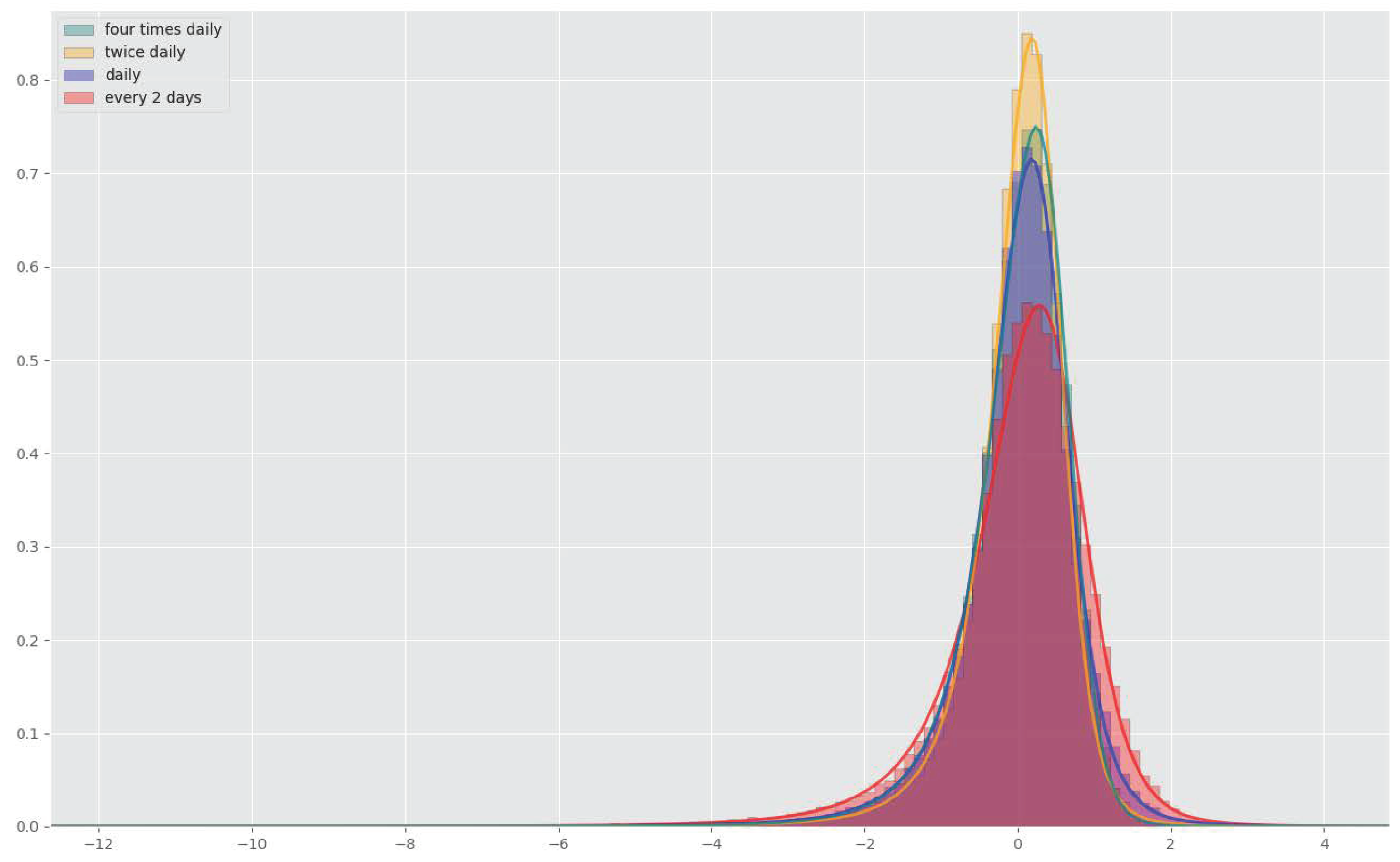
We implement deep hedges on rBergomi paths with the Hurst parameter H = 0.10 , where we re-hedged from every two days, up to four times a day. Again, one can see in Figure 7 that the distribution became slightly less leptocurtic, with more frequent rebalancing. The quadratic losses also decreased with higher frequency (see Table 4). However, this seems to happen at a slower rate than expected. This would essentially mean that as soon as transaction costs are present, small gains from more frequent rebalancing would be completely outweighed by higher transaction fees. As a matter of fact, for the four-time daily re-hedge the loss slightly increased, which indicates the model once again saturates, this time with respect to the hedging frequency. This is quite surprising considering higher hedging frequency usually translates to better performance in a continuous models. This is because the approximation is getting closer and closer to the continuous setting.
Behaviour of distributions as well as hedging losses is in fact quite reminiscent of the behaviour of jump diffusion models analysed by Sepp (2012), which we recall in the following section.

4.3. Relation to the Literature

It is rather interesting that Sepp (2012) observes a similar behaviour when delta hedging under jump diffusion models. Similarly to our observations above, he finds (in the presence of jumps) that after a certain point the volatility of the P&L cannot be reduced by increasing the hedging frequency. More precisely, he shows that for jump diffusion models, there is a lower bound on the volatility of the P&L in relation to the hedging frequency. Not only that, the P&L distributions in Figure 8 for delta hedges under jump diffusion models are generally fairly similar to ours.
This gives us the idea to treat the discretised rough models as jump models. In this case, the market is incomplete, and it is not possible to perfectly hedge a contingent claim with a portfolio containing a finite number of instruments (He et al. 2007). In practice, traders try to come as close as possible to the perfect hedge by trading a number of different options.
Unfortunately, when trying to implement the hedge approximation, we are quickly faced with the absence of analytical pricing formulas and limitations of the slow Monte-Carlo scheme. In order for us to train the deep hedge, we would have to calculate option prices on every time step of each sample path. In a typical application, we would need around 10 options with different strikes and at least 10 5 sample paths.

5. Conclusions

In this work, we presented and compared different methods for hedging under rough volatility models. More specifically, we analysed and implemented the perfect hedge for the rBergomi model from (Viens and Zhang 2019) and used the deep hedging scheme from (Buehleret al. 2019), which had to be adapted to a non-Markovian framework.
We were particularly interested in the dependence of the P&L on the Hurst parameter. We conclude that the deep hedge with the proposed architecture performs better than the discretised perfect hedge for all H. We also find that the hedging P&L distributions for low H are highly left-skewed and have a lot of mass in the left tail under the model hedge as well as the deep hedge.
To mitigate the heavy losses in cases when H is close to zero, we explored increasing the hedging frequency up to four times a day. The loss did improve and the P&L distribution became less leptocurtic, however only slightly. Intriguingly, slow response to increased hedging frequency and left-skewed P&L distribution are characteristic of delta hedges under jump diffusion models (Sepp 2012). We therefore observe that in terms of hedging, there is a relation between jump diffusion models and rough models. In accordance with the literature, we find that the price process, despite being a continuous martingale, exhibits jump-like behaviour (McCrickerd and Pakkanen 2018). We believe this is an excellent illustration of rough volatility models dynamics. Explosive, almost jump-like patterns in the stock price might be the reason why they can fit the short end of implied volatility so well.
In our view, it is crucial to take into account the jump aspect, when looking for an optimal hedge in discretised rough volatility models. Our suggestion for future research is adapting the objective function in the deep hedge scheme for jump risk optimisation. The first step would be optimisation of the expected shortfall risk measure. Next, more appropriate jump risk measures for discretised rough models can be developed. These risk measures cannot be completely analogous to the risk measures in (Sepp 2012), since rough models themselves do not feature jumps.

Author Contributions

All authors contributed to the conception of the manuscript. All authors have read and agreed to the published version of the manuscript.

Funding

We gratefully acknowledge support by ETH Foundation and SNF project 179114.

Institutional Review Board Statement

Not applicable.

Informed Consent Statement

Not applicable.

Data Availability Statement

Not applicable.

Conflicts of Interest

The authors declare no conflict of interest.

Appendix A. Path Derivatives

Denote by D 0 a càdlàg space and by D t and C t the space of càdlàg functions on [ t , T ] and the space of continuous functions on [ t , T ] , respectively. Additionally, we denote by ω the sample paths on [ 0 , T ] , with ω t as its value at time t and define
Λ : = [ 0 , T ] × C ( [ 0 , T ] , R d ) , Λ ¯ : = ( t , ω ) [ 0 , T ] × D 0 : ω | [ t , T ] C ; ω T : = sup t [ 0 , T ] | ω t | , d ( t , ω ) , ( t , ω ) : = | t t | + ω ω T .
Furthermore, we denote the set of all d -continuous functions u : Λ ¯ R by C ( Λ ¯ ) . Define the usual horizontal time derivative for u C ( Λ ¯ ) as in (Dupire 2019):
t u ( t , ω ) : = lim δ 0 u ( t + δ , ω ) u ( t , ω ) δ for all ( t , ω ) Λ ¯ ,
requiring of course that the limit exists. For the spatial derivative with respect to ω , however, we use the definition of the Gateaux derivative for any ( t , ω ) Λ ¯ :
ω u ( t , ω ) , η = lim ε 0 u ( t , ω + ε η 1 [ t , T ] ) u ( t , ω ) ε for any η C t .
Note that the function u ( t , · ) in the definition of the derivative is “lifted” only on [ t , T ] and not on [ 0 , t ) . Hence, the convention we follow is actually
ω u ( t , ω ) , η : = ω u ( t , ω ) , η 1 [ t , T ] for any s < t and η C s .
The definition of Gateaux derivative is clearly also equal to
ω u ( t , ω ) , η = d d ε u ( t , ω + ε η 1 [ t , T ] ) ϵ = 0 .
Remark A1.
We remark that our definition of the spatial derivative is different from the one in (Cont and Fournié 2013; Dupire 2019), where functional derivative quantifies the sensitivity of the functional to the variation solely in the end point of the path, i.e., ω t . While in our definition, the perturbation takes place throughout the whole interval [ t , T ] .
We define two more spaces necessary for our analysis:
C 1 , 2 ( Λ ¯ ) : = u C ( Λ ¯ ) : φ C ( Λ ¯ ) for φ { t u , ω u , ω ω 2 u } , C + 1 , 2 ( Λ ¯ ) : = u C ( Λ ¯ ) : φ has polynomial growth for φ { t u , ω u , ω ω 2 u } and ω ω 2 u , ( η , η ) is locally uniformly continuous in ω with polynomial growth .

Appendix B. Functional Itô Formula

We have to differentiate two cases. The regular case where H ( 1 2 , 1 ) and the singular case where the coefficients b, σ explode, because of the power-kernel in Riemann–Liouville fractional Brownian motion whenever the Hurst exponent H lies in ( 0 , 1 2 ) . In the singular case, the coefficients b , σ C t , and thus they cannot serve as the test function in the right side of (A2), since Gateaux derivative would not make sense any more. In order to develop an Itô formula for the singular case, definitions need to be slightly amended. Nonetheless, Viens et al. show that both cases yield a similar functional Itô formula.
Assumption A1.
i 
The SDE (5) admits a weak solution ( X , W ) .
ii 
E sup t [ 0 , T ] X t p < for all p 1 .
Assumption A2.
i 
(Regular case) For any r [ 0 , T ] , t b ( t ; r , · ) , t σ ( t ; r , · ) exist for t [ r , T ] and for φ = b , σ , t b , t σ ,
| φ ( t ; r , ω ) | C 0 ( 1 + ω T κ 0 ) C 0 , κ 0 > 0 .
ii 
(Singular case) For any r [ 0 , T ] , t ( t ; r , · ) exists for t ( r , T ] with φ = b , σ . There exists H ( 0 , 1 2 ) s.t., for some C 0 , κ 0 > 0
| φ ( t ; r , ω ) | C 0 ( 1 + ω T κ 0 ) ( t r ) H 1 2 and | φ t ( t ; r , ω ) | C 0 ( 1 + ω T κ 0 ) ( t r ) H 3 2
Theorem A1
(Functional Itô formula). Let X be a weak solution to the SDE (5) for which E sup t [ 0 , T ] X t p < for all p 1 and Assumption A2 hold. Then
d u ( t , X t Θ t ) = t u ( t , X t Θ t ) d t + 1 2 ω ω u ( t , X t Θ t ) , ( σ t , X , σ t , X ) d t + ω u ( t , X t Θ t ) , b t , X d t + ω u ( t , X t Θ t ) , σ t , X d W t , P - a . s .
for u C + 1 , 2 ( Λ ) in the regular case and u C + , β 1 , 2 ( Λ ) with regularised Gateaux derivative for the singular case. For φ = b , σ the notation φ s t , ω : = φ ( s ; t , ω ) only emphasises the dependence on s [ t , T ] . For the definition of C + , β 1 , 2 ( Λ ) and precise statement of the theorem in the singular case, see Theorem 3.17 and Theorem 3.10 in (Viens and Zhang 2019)

Appendix C. Discretisation of the Gateaux Derivative

It can be easily shown that Θ ^ s t = f ( Θ s t ) for some f : R R . Therefore, we have a direct relation between the auxiliary process Θ and the forward variance Θ ^ , which allows us to write the option price as the function of the entire forward variance curve Θ ^ [ t , T ] t at time t [ 0 , T ] , namely u ( t , S t , Θ [ t , T ] t ) = u ˜ ( t , S t , Θ ^ [ t , T ] t ) . This is important, when performing Monte-Carlo, since in the rough Bergomi model, the forward variance curve is directly modelled in the variance process with ξ t ( · ) = Θ ^ · t .
Let us suppose that we are able to trade at times 0 = t 0 < t 1 < < t n = T . In order to get the hedging weights at trading times t i , we have to discretise the derivatives. The Gateaux derivative with respect to the stock simplifies to the usual derivative, and the discretisation is straightforward:
x u ˜ ( t , S t , Θ ^ [ t , T ] t ) u ˜ ( t , S t + ε , Θ ^ [ t , T ] t ) u ˜ ( t , S t , Θ ^ [ t , T ] t ) ε for small ε > 0 .
For the path-wise derivative, the discretisation is not immediately obvious, especially because of the dependence of the option price u ˜ at time t on functional over the whole interval [ t , T ] , more precisely since u : [ 0 , T ] × [ 0 , ) × C ( [ 0 , T ] R ) . First, we remind ourselves of the definition of the Gateaux derivative on a path ω :
ω u ( t , ω ) , η = lim ε 0 u ( t , ω + ε η 1 [ t , T ] ) u ( t , ω ) ε for any η Ω t .
We proceed as in (Jacquier and Oumgari 2019) by approximating Θ ^ [ t , T ] t as a piecewise constant function
Θ ^ s t i I Θ ^ i t 1 [ t i , t i + 1 ) ( s ) a i t = a s t 1 [ t i , t i + 1 ) ( s ) ,
where I : = { i N : t t i T } . We introduce the following approximations of the path derivatives along the direction a t :
ω u ˜ ( t , S t , Θ ^ [ t , T ] t ) , a t ε u ˜ t , S t , i I ( Θ ^ i t + ε a t ) 1 [ t i , t i + 1 ) ( s ) s [ t , T ] ε = 0 = ε u ^ t , S t , Θ ^ i t + ε a i t i I ε = 0 = i I Θ ^ i t u ^ ( t , S t , θ t ) a i t ,
with θ t : = ( Θ ^ i t ) i I and u ^ acts on [ 0 , T ] × [ 0 , ) × R # I . Further discretising the derivative, we have for the flat forward variance ξ ( t ) = ξ 0 :
ω u ˜ ( t , S t , ξ 0 ) , a t u ˜ ( t , S t , ξ 0 + ε ) u ˜ ( t , S t , ξ 0 ) ε a t for small ε > 0 .
The option prices u ˜ can now be evaluated using Monte-Carlo at each time step to get the hedging weights. Note that the discretisation of the Gateaux derivative is purely heuristic and that a rigorous proof of the convergence to the true derivative is out of scope of this work. For more details we refer to (Jacquier and Oumgari 2019).

Notes

1
For the numerical implementation of the resulting strategies that we consider in the following sections, we naturally consider again the discrete filtration introduced above in Section 2, representing a discretisation of the continuous market.
2
Several estimation procedures of the Hurst parameter were used; see, e.g., (Di Matteo 2007; Di Matteoet al. 2005). Estimations of the paths simulated with the hybrid scheme (Bennedsenet al. 2017; McCrickerd and Pakkanen 2018) were on the other hand in alignment with the input parameter.
3
Note that by completely recurrent we do not mean the same network is used at each time step, but that the hidden state is passed on to the cell in the next time step along with current portfolio positions.
4
For Heston parameters α = 1 , b = 0.04 , σ = 0.8 , V 0 = 0.04 , S 0 = 100 and ρ = 0.7 the quadratic losses were 0.20 under original architecture and 0.162 under the fully recurrent one. Both training times were fairly similar as well.
5
All the experiments were performed on a Dell-HQIQ2UV laptop with Intel i7-8550U CPU using TensorFlow v1.3.

References

  1. Alòs, Elisa, Jorge A. León, and Josep Vives. 2007. On the short-time behavior of the implied volatility for jump-diffusion models with stochastic volatility. Finance and Stochastics 11: 571–89. [Google Scholar] [CrossRef] [Green Version]
  2. Bayer, Christian, Blanka Horvath, Aitor Muguruza, Benjamin Stemper, and Mehdi Tomas. 2019. On deep calibration of (rough) stochastic volatility models. arXiv arXiv:1908.08806. [Google Scholar]
  3. Bayer, Christian, Peter Friz, and Jim Gatheral. 2015. Pricing under rough volatility. Quantitative Finance 16: 887–904. [Google Scholar] [CrossRef]
  4. Bennedsen, Mikkel, Asger Lunde, and Mikko S. Pakkanen. 2017. Hybrid scheme for brownian semistationary processes. Finance and Stochastics 21: 931–65. [Google Scholar] [CrossRef] [Green Version]
  5. Benth, Fred Espen, Nils Detering, and Silvia Lavagnini. 2020. Accuracy of deep learning in calibrating HJM forward curves. arXiv arXiv:2006.01911. [Google Scholar]
  6. Bolko, Anine E., Kim Christensen, Mikko S. Pakkanen, and Bezirgen Veliyev. 2020. Roughness in spot variance? A GMM approach for estimation of fractional log-normal stochastic volatility models using realized measures. arXiv arXiv:2010.04610. [Google Scholar]
  7. Buehler, Hans, Blanka Horvath, Terry Lyons, Imanol Perez Arribas, and Ben Wood. 2020a. A data-driven market simulator for small data environments. SSRN Electronic Journal. [Google Scholar] [CrossRef]
  8. Buehler, Hans, Blanka Horvath, Terry Lyons, Imanol Perez Arribas, and Ben Wood. 2020b. Generating financial markets with signatures. SSRN Electronic Journal. [Google Scholar] [CrossRef]
  9. Buehler, Hans, Lukas Gonon, Josef Teichmann, and Ben Wood. 2019. Deep hedging. Quantitative Finance 19: 1271–91. [Google Scholar] [CrossRef]
  10. Carmona, Philippe, Gérard Montseny, and Laure Coutin. 1998. Application of a Representation of Long Memory Gaussian Processes. Publications du Laboratoire de statistique et probabilités. Toulouse: Laboratoire de Statistique et Probabilités. [Google Scholar]
  11. Cont, Rama, and David-Antoine Fournié. 2013. Functional itô calculus and stochastic integral representation of martingales. The Annals of Probability 41: 109–33. [Google Scholar] [CrossRef]
  12. Cuchiero, Christa, Martin Larsson, and Josef Teichmann. 2020. Deep neural networks, generic universal interpolation, and controlled ODEs. SIAM Journal on Mathematics of Data Science 2: 901–19. [Google Scholar] [CrossRef]
  13. Cuchiero, Christa, Wahid Khosrawi, and Josef Teichmann. 2020. A generative adversarial network approach to calibration of local stochastic volatility models. Risks 8: 101. [Google Scholar] [CrossRef]
  14. Di Matteo, Tiziana. 2007. Multi-scaling in finance. Quantitative Finance 7: 21–36. [Google Scholar] [CrossRef]
  15. Di Matteo, Tiziana, Tomaso Aste, and Michel M. Dacorogna. 2005. Long-term memories of developed and emerging markets: Using the scaling analysis to characterize their stage of development. Journal of Banking & Finance 29: 827–51. [Google Scholar]
  16. Dupire, Bruno. 2019. Functional itô calculus. Quantitative Finance 19: 721–29. [Google Scholar] [CrossRef]
  17. Fukasawa, Masaaki. 2010. Asymptotic analysis for stochastic volatility: Martingale expansion. Finance and Stochastics 15: 635–54. [Google Scholar] [CrossRef] [Green Version]
  18. Föllmer, Hans, and Alexander Schied. 2016. Stochastic Finance: An Introduction in Discrete Time. New York: De Gruyter. [Google Scholar]
  19. Gassiat, Paul. 2019. On the martingale property in the rough bergomi model. Electronic Communications in Probability 24. [Google Scholar] [CrossRef]
  20. Gatheral, Jim, Thibault Jaisson, and Mathieu Rosenbaum. 2018. Volatility is rough. Quantitative Finance 18: 933–49. [Google Scholar] [CrossRef]
  21. Gierjatowicz, Patryk, Marc Sabate-Vidales, David Šiška, Lukasz Szpruch, and Žan Žurič. 2020. Robust pricing and hedging via neural SDEs. SSRN Electronic Journal. [Google Scholar] [CrossRef]
  22. He, Changhong, J. Shannon Kennedy, Thomas F. Coleman, Peter A. Forsyth, Yuying Li, and Kenneth R. Vetzal. 2007. Calibration and hedging under jump diffusion. Review of Derivatives Research 9: 1–35. [Google Scholar] [CrossRef] [Green Version]
  23. Henry-Labordere, Pierre. 2019. Generative models for financial data. SSRN Electronic Journal. [Google Scholar] [CrossRef]
  24. Hernandez, Andres. 2016. Model calibration with neural networks. Risk. [Google Scholar] [CrossRef] [Green Version]
  25. Hochreiter, Sepp, and Jürgen Schmidhuber. 1997. Long short-term memory. Neural Computation 9: 1735–80. [Google Scholar] [CrossRef] [PubMed]
  26. Horvath, Blanka, Aitor Muguruza, and Mehdi Tomas. 2021. Deep learning volatility: A deep neural network perspective on pricing and calibration in (rough) volatility models. Quantitative Finance 21: 1. [Google Scholar] [CrossRef]
  27. Ilhan, Aytaç, Mattias Jonsson, and Ronnie Sircar. 2009. Optimal static-dynamic hedges for exotic options under convex risk measures. Stochastic Processes and their Applications 119: 3608–32. [Google Scholar] [CrossRef] [Green Version]
  28. Jacquier, Antoine, and Mugad Oumgari. 2019. Deep curve-dependent pdes for affine rough volatility. arXiv arXiv:1906.02551. [Google Scholar]
  29. Kac, Mark. 1949. On distributions of certain wiener functionals. Transactions of the American Mathematical Society 65: 1–13. [Google Scholar] [CrossRef]
  30. Kondratyev, Alexei, and Christian Schwarz. 2019. The market generator. Econometrics: Econometric & Statistical Methods - Special Topics eJournal. [Google Scholar] [CrossRef]
  31. Liu, Shuaiqiang, Anastasia Borovykh, Lech A. Grzelak, and Cornelis W. Oosterlee. 2019. A neural network-based framework for financial model calibration. Journal of Mathematics in Industry 9: 9. [Google Scholar] [CrossRef]
  32. Livieri, Giulia, Saad Mouti, Andrea Pallavicini, and Mathieu Rosenbaum. 2018. Rough volatility: Evidence from option prices. IISE Transactions 50: 767–76. [Google Scholar] [CrossRef]
  33. McCrickerd, Ryan, and Mikko S. Pakkanen. 2018. Turbocharging monte carlo pricing for the rough bergomi model. Quantitative Finance 18: 1877–86. [Google Scholar] [CrossRef] [Green Version]
  34. Pascanu, Razvan, Caglar Gulcehre, Kyunghyun Cho, and Yoshua Bengio. 2014. How to construct deep recurrent neural networks. Paper presented at Second International Conference on Learning Representations, ICLR 2014, Banff, AB, Canada, April 14–16. [Google Scholar]
  35. Ruf, Johannes, and Weiguan Wang. 2020. Neural networks for option pricing and hedging: A literature review. The Journal of Computational Finance 24. [Google Scholar] [CrossRef]
  36. Schweizer, Martin. 1995. Variance-optimal hedging in discrete time. Mathematics of Operations Research 20: 1–32. [Google Scholar] [CrossRef]
  37. Sepp, Artur. 2012. An approximate distribution of delta-hedging errors in a jump-diffusion model with discrete trading and transaction costs. Quantitative Finance 12: 1119–41. [Google Scholar] [CrossRef]
  38. Viens, Frederi, and Jianfeng Zhang. 2019. A martingale approach for fractional brownian motions and related path dependent PDEs. The Annals of Applied Probability 29: 3489–540. [Google Scholar] [CrossRef] [Green Version]
  39. Wiese, Magnus, Lianjun Bai, Ben Wood, and Hans Buehler. 2019. Deep hedging: Learning to simulate equity option markets. arXiv arXiv:1911.01700. [Google Scholar] [CrossRef] [Green Version]
  40. Wiese, Magnus, Robert Knobloch, Ralf Korn, and Peter Kretschmer. 2020. Quant GANs: Deep generation of financial time series. Quantitative Finance 20: 1419–40. [Google Scholar] [CrossRef] [Green Version]
  41. Xu, Mingxin. 2005. Risk measure pricing and hedging in incomplete markets. Annals of Finance 2: 51–71. [Google Scholar] [CrossRef]
  42. Xu, Tianlin, Li K. Wenliang, Michael Munn, and Beatrice Acciaio. 2020. Cot-gan: Generating sequential data via causal optimal transport. arXiv arXiv:2006.08571. [Google Scholar]
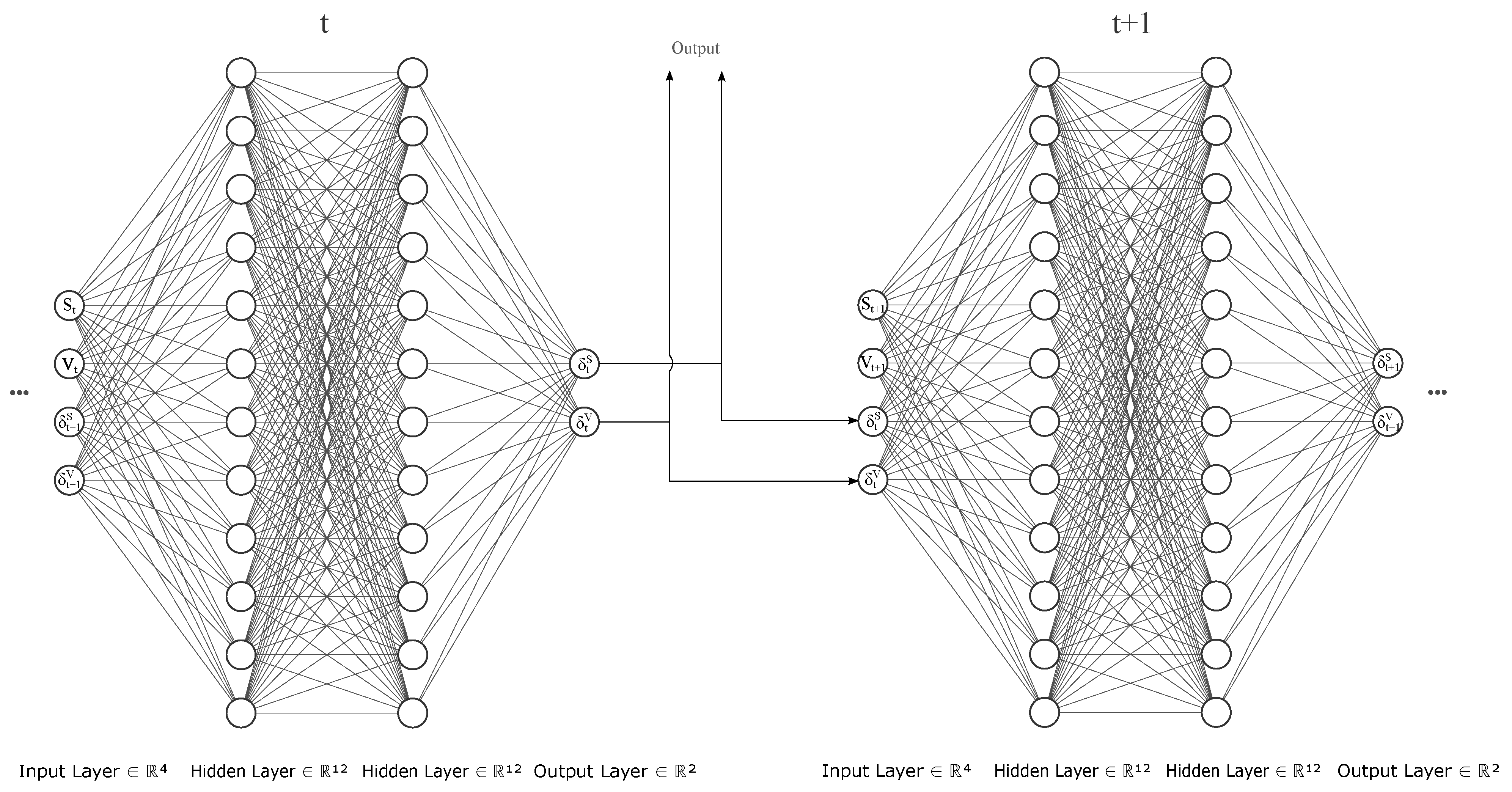
Figure 1. Original Network Archiecture.
Risks 09 00138 g001
Figure 2. rBergomi model hedge (blue) compared to the deep hedge (red) trained on 75 epochs on rBergomi paths with H = 0.10 . Note that the option price is only p 0 = 2.39 and that such a hedge can result in a substantial loss.
Risks 09 00138 g002
Figure 3. Fully Recurrent Neural Network (fRNN) Architecture. The recurrent structure of this architecture is clearly visible as hidden states are passed on to the next cell at each time step.
Risks 09 00138 g003
Figure 4. Empirical P&L distributions in log-scale for different Hurst parameters under the fRNN hedge. Loss on test denotes the realised quadratic loss on the test set for a network trained on 75 epochs.
Risks 09 00138 g004
Figure 5. Under the discretised rough Bergomi model, the stock can jump by more than ± 30 % in a single time step. This stock path caused extreme loss of 27.73 seen in Figure 4.
Risks 09 00138 g005
Figure 6. P&L distributions of rBergomi model hedge (red) vs. deep hedge with proposed architecture (blue) for different Hurst parameters realised on 10 3 sample paths.
Risks 09 00138 g006
Figure 7. fRNN deep hedge for different hedging frequencies (with H = 0.10 ). The plot was rescaled, because of the massive outliers in the two day rehedge case. Non-central t distribution was fit for better visiblity.
Risks 09 00138 g007
Figure 8. Profit and loss distributions for delta hedging under jump diffusion models (JDM) from (Sepp 2012).
Risks 09 00138 g008
Table 1. Comparison of the quadratic loss between model and deep hedges trained 75 epochs for different H.
Quadratic Hedging Loss
H Model HedgeDeep Hedge
0.10 1.451.16 (*1.12)
0.20 0.520.67
0.30 0.340.46
0.40 0.240.36
*—on 200 epochs.
Table 2. Quadratic loss for different Hurst parameters. Run time on 75 epochs was approximately 2 h for each parameter.
Hurst Parameter
H 0.10 0.20 0.30 0.40 0.60 0.70 0.80 0.90
Quad. loss0.834 (*0.628)0.3760.2630.2440.2040.2060.1970.191
*—loss on 200 epochs.
Table 3. Comparison of the quadratic loss between model and deep hedges with fRNN architecture trained on 75 epochs for different H.
Quadratic Hedging Loss
H Model HedgeDeep HedgeDeep Hedge—fRNN
0.10 1.451.16 (*1.12)0.83 (*0.63)
0.20 0.520.670.38
0.30 0.340.460.26
0.40 0.240.360.22
*—on 200 epochs.
Table 4. Comparison of the fRNN deep hedge quadratic losses for different hedging frequencies (with H = 0.10 ).
Rehedging Frequency
H = 0 . 10 Every Two DaysDailyTwice DailyFour Times Daily
Quadratic loss1.110.650.460.52
Training time (h)3.17.519.645.3
Publisher’s Note: MDPI stays neutral with regard to jurisdictional claims in published maps and institutional affiliations.