The Combined Stop-Loss and Quota-Share Reinsurance: Conditional Tail Expectation-Based Optimization from the Joint Perspective of Insurer and Reinsurer

Abstract

In the presence of reinsurance, an insurer may effectively reduce its (aggregated) loss by partially ceding such a loss to a reinsurer. Stop-loss and quota-share reinsurance contracts are commonly agreed between these two parties. In this paper, we aim to explore a combination of these contracts. The survival functions of the ceded loss and the retained loss are firstly investigated. Optimizing such a reinsurance design is then carried out from the joint perspective of the insurer and the reinsurer. Specifically, we explicitly derive optimal retentions under a criterion of minimizing a convex combination of conditional tail expectations of the insurer’s total loss and the reinsurer’s total loss. In addition, an estimation procedure and more explanations on numerical examples are also presented to find their estimated values.

1. Introduction

Under a reinsurance contract, a loss faced by an insurer is partially ceded to a reinsurer. As a consequence, the insurer is liable for the remaining loss, called the retained loss, and a fixed reinsurance premium, which has to be paid to the reinsurer. Meanwhile, the liability of the reinsurer is the ceded loss subtracted by the reinsurance premium. However, as noted by Cai and Tan (2007), there is a classic trade-off between the retained loss and the ceded loss. When the loss ceded to the reinsurer is too large, the reinsurance premium charged will also be too high. On the other hand, reducing the reinsurance premium will make the insurer retain a potentially large loss. Accordingly, the insurer needs a reinsurance with optimal design.

Optimizing the reinsurance design from the perspective of the insurer has been carried out by many researchers using various approaches. For instance, Gajek and Zagrodny (2000) considered an optimization criterion of minimizing the variance of the loss retained by the insurer. Meanwhile, Kaluszka (2004) obtained optimal reinsurance arrangements through a mean-variance approach. More recently, Cai and Tan (2007) derived optimal retentions for a stop-loss reinsurance as the solutions to the minimization of value-at-risk (VaR) and conditional tail expectation (CTE) of the insurer’s total loss. As demonstrated by Cai et al. (2008) under these two risk measures, the optimal reinsurance can be in the form of stop-loss, quota-share, or their combination. The optimization on the former two reinsurance contacts was investigated further by Tan et al. (2009) who also employed the VaR- and CTE-based criteria. Several extensions of the stop-loss reinsurance, such as limited stop-loss and truncated stop-loss, were derived as the solutions to the optimization problem of Chi and Tan (2011) under the VaR and conditional VaR (CVaR) risk measures. In particular, optimal parameters for the limited stop-loss reinsurance were found by Zhou et al. (2015). Meanwhile, Zhou et al. (2011) and Putri et al. (2021) investigated the optimality of the combination of quota-share and stop-loss reinsurance. The other studies on the reinsurance optimization from the insurer’s viewpoint under the above risk measures may be found in Lu et al. (2014), Lu et al. (2016), Du et al. (2019), and Hu et al. (2021). In contrast, optimizing the reinsurance treaty from the perspective of a reinsurer was undertaken by Tan et al. (2020). Specifically, they minimized the VaR and the CTE of the reinsurer’s total loss.

An optimal form of reinsurance from the insurer’s perspective, however, may not meet the reinsurer’s goal, and vice versa. In order to derive the optimal reinsurance accepted by both the insurer and the reinsurer, another approach is required to optimize an objective function constructed from their joint perspective. For instance, a criterion of maximizing the joint survival probability and the joint profitable probability from the perspective of both the insurer and the reinsurer was proposed by Cai et al. (2013). Based on the results in Cai et al. (2013), Fang and Qu (2014) derived optimal retentions for a combination of quota-share and stop-loss reinsurance by maximizing the joint survival probability. In addition to employing the joint survival probability, other criteria were also taken into consideration by Zhang et al. (2018) to determine an optimal retention level of a quota-share reinsurance. Such optimization criteria include minimizing the total variance, the total VaR, and the total tail-VaR (TVaR) of the insurer’s loss and the reinsurer’s loss.

To ensure that reducing the loss from one party can not be carried out without increasing the loss from another party, a convex combination of the risk measures of the losses for both parties was recently utilized by several authors instead of just summing them. For instance, Cai et al. (2016) suggested an optimization criterion of minimizing a convex combination of VaRs of the insurer’s total loss and the reinsurer’s total loss. In particular, Liu and Fang (2018) implemented this approach on their study to obtain optimal parameters for the quota-share and stop-loss reinsurance designs. More recently, the above optimization criterion was also adopted by Jiang et al. (2017), Fang et al. (2019), and Chen and Hu (2020) by using the same VaR risk measure. They found that the combined stop-loss and quota-share reinsurance is one of the optimal solutions to their optimization problems.

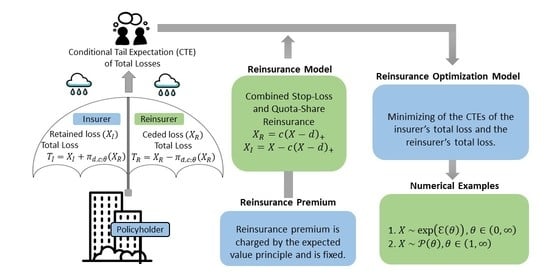
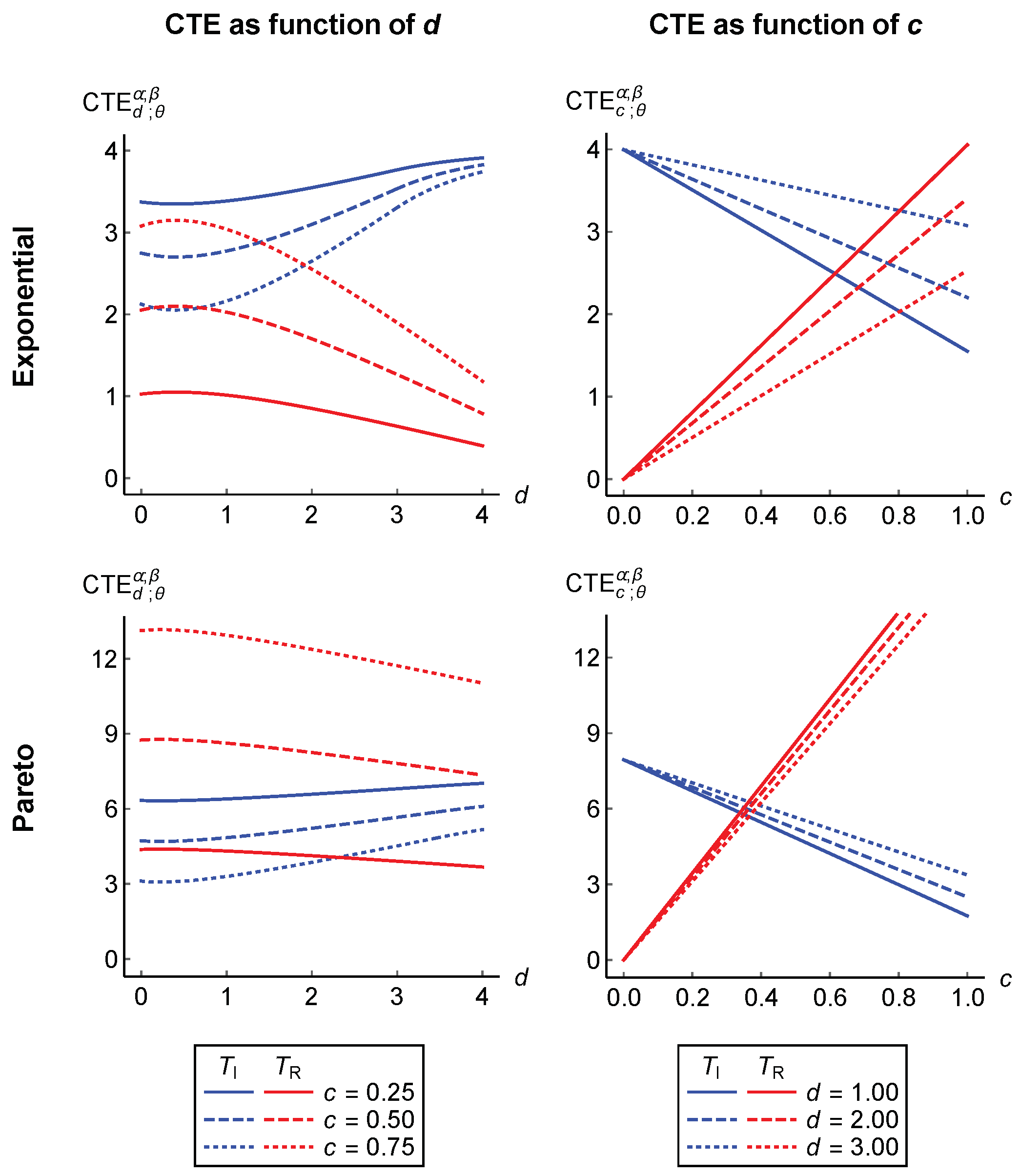
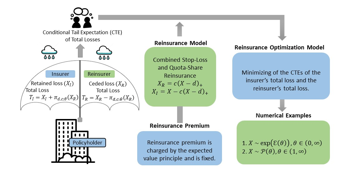
In this paper, we aim to explore the combined stop-loss and quota-share reinsurance. We study, in Section 2, the survival function of the loss ceded to the reinsurer and that of the loss retained by the insurer in the presence of this reinsurance contract. In Section 3, we then optimize the combined stop-loss and quota-share reinsurance from the joint perspective of the insurer and the reinsurer by developing a new optimization criterion similar to Jiang et al. (2017), Fang et al. (2019), and Chen and Hu (2020). Instead of using the probability-based risk measure of VaR, an alternative risk measure of CTE is employed to overcome its weaknesses by taking into account the magnitude of the losses beyond the VaR (Syuhada et al. 2021). Specifically, we derive explicit expressions of optimal retentions for the reinsurance we design by minimizing a convex combination of CTEs of the insurer’s total loss and the reinsurer’s total loss. An estimation for the resulting optimal retentions is also presented in Section 4 with numerical examples when the initial loss faced by the insurer is assumed to follow an exponential or Pareto distribution. Section 5 concludes our study.

2. Combined Stop-Loss and Quota-Share Reinsurance

Let X be loss or risk transferred from an insured to an insurer. This loss may be an aggregate of individual losses that form an insurance portfolio. In this paper, the loss X is assumed to be a non-negative random variable with survival function $S_{X;\theta }(x)=\mathbb{P}(X>x)$ determined by a parameter $\theta \in \Omega$, where $\Omega$ denotes a parameter space. We also assume that $S_{X;\theta }$ is continuous and strictly decreasing on the interval $(0,\infty )$ with a possible jump at $x=0$. Consequently, the inverse function $S_{X;\theta }^{-1}$ exists on the interval $\left(0,S_{X;\theta }(0)\right)$. In addition, the expectation of X, $\mathbb{E}(X)$, is assumed to be finite. Its value may be computed from the survival function $S_{X;\theta }$ through integration, i.e.,

$$\mathbb{E}(X)={\int }_0^{\infty }{S}_{X;\theta }(x)\mathrm{d}x.$$

For illustration purposes throughout this paper, we follow a suggestion of Burnecki et al. (2021) assuming an exponentially distributed loss $X\sim \mathcal{E}(\theta )$ with survival function

$$S_{X;\theta }(x)=\left\{\begin{array}{cc}1,\hfill & x<0,\hfill \\ {\mathrm{e}}^{-\theta x},\hfill & x\ge 0,\hfill \end{array}\right.$$

(1)

where $\theta \in (0,\infty )$, which is equal to the reciprocal of its mean. As a comparison, we may also assume X to follow a Pareto distribution, $\mathcal{P}(\theta )$, with a heavier tail. Its survival function is defined as follows:

$$S_{X;\theta }(x)=\left\{\begin{array}{cc}1,\hfill & x<0,\hfill \\ {(1+x)}^{-\theta },\hfill & x\ge 0.\hfill \end{array}\right.$$

(2)

Its parameter, $\theta$, denoting the tail index belongs to $(1,\infty )$. This consideration is to make sure that its mean, ${(\theta -1)}^{-1}$, exists.

Under a reinsurance designed in a fixed time period, the insurer decides to reduce the loss X by ceding the part of X, say $L_{\mathrm{R}}(X)$ for a function $L_{\mathrm{R}}:[0,\infty )\to [0,\infty )$ satisfying $0\le L_{\mathrm{R}}(x)\le x$, for all $x\in [0,\infty )$, to a reinsurer. Meanwhile, the remaining loss of size $L_{\mathrm{I}}(X)$, where $L_{\mathrm{I}}:[0,\infty )\to [0,\infty )$ with $L_{\mathrm{I}}(x)=x-L_{\mathrm{R}}(x)$, for all $x\in [0,\infty )$, is retained by the insurer. In other words, in the presence of reinsurance contract, the initial loss X is split into two parts such that $X=L_{\mathrm{R}}(X)+L_{\mathrm{I}}(X)$. We then use the notations $X_{\mathrm{R}}=L_{\mathrm{R}}(X)$ and $X_{\mathrm{I}}=L_{\mathrm{I}}(X)$ to denote those parts. We call them ceded loss and retained loss, respectively, whilst the functions $L_{\mathrm{R}}(x)$ and $L_{\mathrm{I}}(x)$ are usually known as ceded loss function and retained loss function, respectively.

When a quota-share reinsurance is designed, the insurer cedes a level c of the initial loss X, i.e., $cX$, to the reinsurer. This means that both the insurer and the reinsurer are involved in facing the loss with unlimited liability (Gray and Pitts 2012). However, the insurer may need to be protected from the potential large loss by retaining the loss up to a limit d only. An excess of size ${(X-d)}_{+}$ is covered by the reinsurer, where $a_{+}=a\vee 0=max\{a,0\}$. This goal may be achieved by designing a stop-loss reinsurance. See Tan et al. (2009) and Liu and Fang (2018) for a more detailed study on those reinsurance contracts.

In this paper, we consider combining the above two reinsurance contracts by firstly setting a retention limit d and, then, affixing a retention level c such that the loss ceded to the reinsurer is given by

$$X_{\mathrm{R}}=c{(X-d)}_{+}=\left\{\begin{array}{cc}0,\hfill & X<d,\hfill \\ c(X-d),\hfill & X\ge d.\hfill \end{array}\right.$$

(3)

The above ceded loss may also be expressed in the form of $c(X-d){\mathbb{I}}_{[d,\infty )}(X)$, where ${\mathbb{I}}_A$ is an indicator function of a set A. Consequently, the insurer is liable for the retained loss of size

$$X_{\mathrm{I}}=X-c{(X-d)}_{+}=\left\{\begin{array}{cc}X,\hfill & X<d,\hfill \\ X-c(X-d),\hfill & X\ge d,\hfill \end{array}\right.$$

(4)

where $a\wedge b$ means $min\{a,b\}$. We call this design a combined stop-loss and quota-share reinsurance. Under this combination, it is obvious that both the ceded loss function $L_{\mathrm{R}}(x)=c{(x-d)}_{+}$ and the retained loss function $L_{\mathrm{I}}(x)=x-c{(x-d)}_{+}$ are increasing with respect to x on $[0,\infty )$. See Figure 1 to investigate their curves.

We see that the pure stop-loss reinsurance is a special case of the above contract for $c=1$. Meanwhile, if the retention limit d is set to be zero, we then have the pure quota-share reinsurance. However, when the value of c is equal to zero, there is no reinsurance and, as a result, the insurer is liable for all the losses. We, in this paper, assume $(d,c)\in (0,\infty )\times (0,1]$ in order to ensure that the insurer truly shares a portion of loss to the reinsurer, instead of retaining all the losses. The notation $(d,c)$ for a pair of d and c is considered to remind us that d is the first retention affixed in designing the combined stop-loss and quota-share reinsurance.

Since the ceded loss $X_{\mathrm{R}}=L_{\mathrm{R}}(X)$ and the retained loss $X_{\mathrm{I}}=L_{\mathrm{I}}(X)$ are the functions of X, their distribution may be determined based on the distribution of X. By employing a simple technique, from Equation (3), the survival function of the ceded loss $X_{\mathrm{R}}$ may be derived as follows:

$$S_{X_{\mathrm{R}};\theta }(x)=\left\{\begin{array}{cc}1,\hfill & x<0,\hfill \\ {\displaystyle S_{X;\theta }\left(\frac{x}{c}+d\right),}\hfill & x\ge 0.\hfill \end{array}\right.$$

(5)

Meanwhile, according to Equation (4), the survival function of $X_{\mathrm{I}}$ is given by

$$S_{X_{\mathrm{I}};\theta }(x)=\left\{\begin{array}{cc}1,\hfill & x<0,\hfill \\ S_{X;\theta }(x),\hfill & 0\le x<d,\hfill \\ {\displaystyle S_{X;\theta }\left(\frac{x-cd}{1-c}\right),}\hfill & x\ge d.\hfill \end{array}\right.$$

(6)

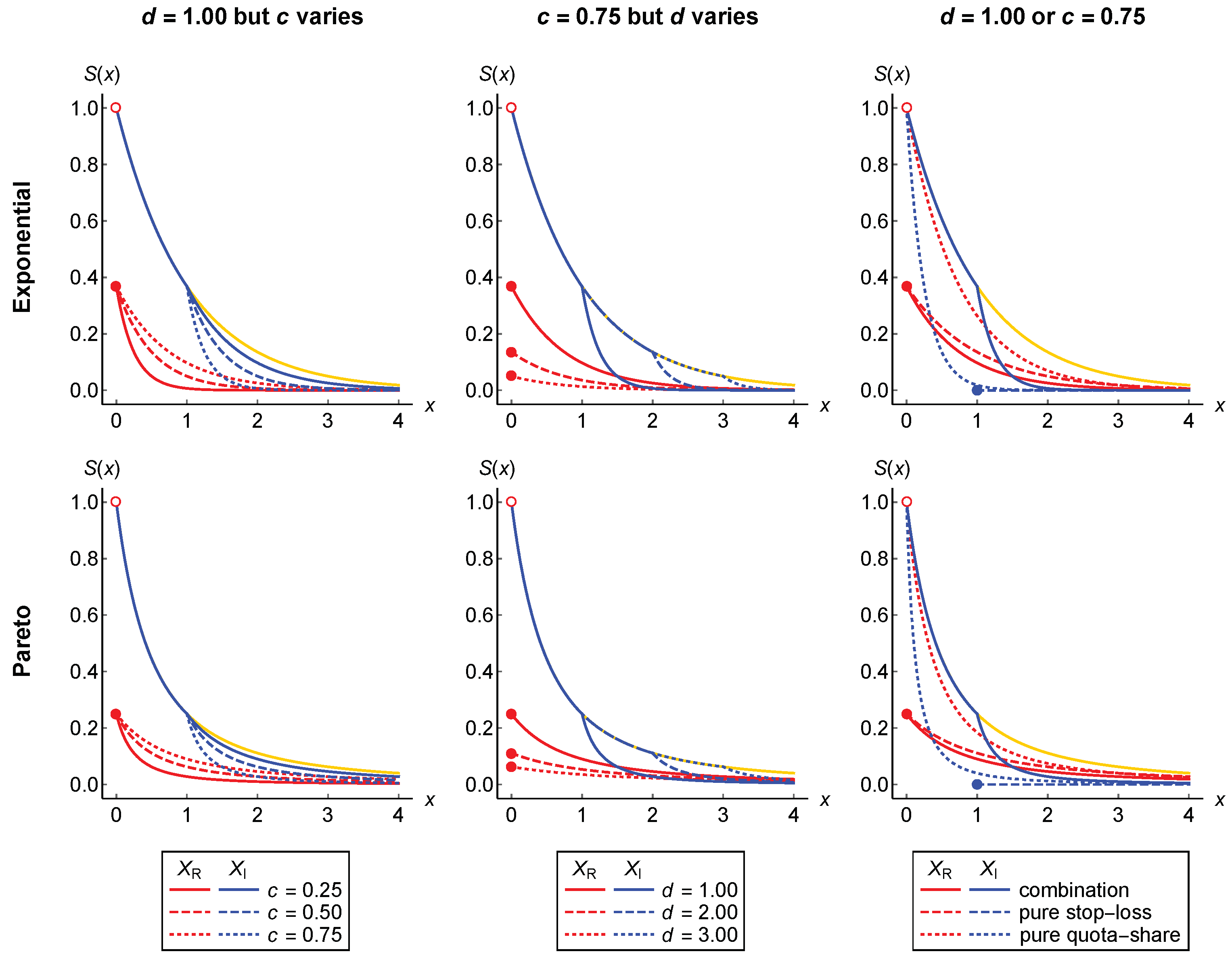
It is obvious that the survival function $S_{X_{\mathrm{R}};\theta }$ is always discontinuous at $x=0$ whilst the discontinuity of $S_{X_{\mathrm{I}};\theta }$ at $x=0$ occurs when the survival function of the initial loss X is discontinuous at this point. In Figure 2, we present their curves for the cases of exponential and Pareto random losses with equal mean, i.e., 1. Their comparison to the curves of the survival functions under the pure stop-loss and pure quota-share reinsurance is also illustrated in this figure.

3. Reinsurance Optimization under CTE Risk Measure

As stated before, in the presence of the (combined stop-loss and quota-share) reinsurance contract, the insurer cedes the part of the loss to the reinsurer. As a consequence, the reinsurance premium of size ${\Pi }_{d,c;\theta }(X_{\mathrm{R}})$ has to be paid by the insurer to the reinsurer. The insurer is thus liable for the total loss $T_{\mathrm{I}}$ defined as the sum of the retained loss $X_{\mathrm{I}}$ and the reinsurance premium ${\Pi }_{d,c;\theta }(X_{\mathrm{R}})$, i.e.,

$$T_{\mathrm{I}}=X_{\mathrm{I}}+{\Pi }_{d,c;\theta }(X_{\mathrm{R}}),$$

(7)

whilst the total loss $T_{\mathrm{R}}$ of the reinsurer is given by

$$T_{\mathrm{R}}=X_{\mathrm{R}}-{\Pi }_{d,c;\theta }(X_{\mathrm{R}}).$$

(8)

In this paper, the reinsurance premium charged by the reinsurer is assumed to be determined by the expected value principle, that is ${\Pi }_{d,c;\theta }^{\beta }(X_{\mathrm{R}})=(1+\beta )\mathbb{E}(X_{\mathrm{R}})$, where $\beta \in (0,\infty )$ is a fixed safety loading factor. Note that the expected value of the ceded loss $X_{\mathrm{R}}$ may be represented by $\mathbb{E}(X_{\mathrm{R}})=c{K}_{\theta }(d)$, where

$$K_{\theta }(d)=\mathbb{E}[{(X-d)}_{+}]={\int }_d^{\infty }{S}_{X;\theta }(x)\mathrm{d}x,$$

therefore the above reinsurance premium may be expressed as below:

$${\Pi }_{d,c;\theta }^{\beta }(X_{\mathrm{R}})=(1+\beta )c{K}_{\theta }(d).$$

(9)

3.1. CTE of Total Losses

When a reinsurance is agreed between the insurer and the reinsurer, the insurer’s objective is actually to manage its risk. In addition to making a profit, the reinsurer also aims to control its own risk ceded from the insurer. A so-called value-at-risk (VaR), widely used in quantitative risk management, may be taken into consideration to measure the potential magnitude of such risks. Basically, VaR is a single value denoting the maximum loss that is likely to occur at a specified $\alpha$ level of significance. For the initial loss X, the VaR is formally defined by

$${\mathrm{VaR}}_{\theta }^{\alpha }(X)=inf\left\{x\in \mathbb{R}:S_{X;\theta }(x)\le \alpha \right\},$$

for all $\alpha \in (0,1)$, which means that the VaR is the $(1-\alpha )$-quantile of the distribution of X. As stated in Section 2, the survival function $S_{X;\theta }$ is assumed to be continuous and strictly decreasing on the interval $\left(0,S_{X;\theta }(0)\right)$. This assumption implies that the inverse function of $S_{X;\theta }$ exists on this interval and, as a result, we obtain

$${\mathrm{VaR}}_{\theta }^{\alpha }(X)=S_{X;\theta }^{-1}(\alpha ),$$

(10)

for all $\alpha \in \left(0,S_{X;\theta }(0)\right)$. Meanwhile, the trivial case, that is ${\mathrm{VaR}}_{\theta }^{\alpha }(X)=0$, occurs for each $\alpha$ belonging to $\left[S_{X;\theta }(0),1\right)$. It is easy to verify that ${\mathrm{VaR}}_{\theta }^{\alpha }(X)$ is strictly decreasing with respect to $\alpha$ on $\left(0,S_{X;\theta }(0)\right)$, which means that, for all ${\alpha }_1,{\alpha }_2\in \left(0,S_{X;\theta }(0)\right)$, we have

$${\alpha }_1<{\alpha }_2\iff {\mathrm{VaR}}_{\theta }^{{\alpha }_2}(X)<{\mathrm{VaR}}_{\theta }^{{\alpha }_1}(X).$$

In fact, the VaR depends only on the probability of the occurrence of the losses and provides no information about the magnitude of the losses that exceed it and may have severe impact (Syuhada et al. 2021). Alternatively, conditional tail expectation (CTE) may be required to correct for these weaknesses. At the $\alpha$ level of significance, the CTE of the loss X is defined as the conditional expectation of X, given all its values exceeding the corresponding VaR, that is

$${\mathrm{CTE}}_{\theta }^{\alpha }(X)=\mathbb{E}[X\mid X>{\mathrm{VaR}}_{\theta }^{\alpha }(X)].$$

This indicates that the CTE is more appropriate than the VaR since it takes into account the magnitude of losses beyond the VaR. Furthermore, the more important advantage of the CTE over the VaR is that the CTE is coherent under suitable conditions whilst the VaR is not since it fails to satisfy the axiom of subadditivity. Note that the CTE and the VaR are related as below:

$$\begin{array}{cc}\hfill {\mathrm{CTE}}_{\theta }^{\alpha }(X)& ={\mathrm{VaR}}_{\theta }^{\alpha }(X)+\mathbb{E}[X-{\mathrm{VaR}}_{\theta }^{\alpha }(X)\mid X>{\mathrm{VaR}}_{\theta }^{\alpha }(X)]\hfill \\ \hfill & ={\mathrm{VaR}}_{\theta }^{\alpha }(X)+\frac{1}{\alpha }{K}_{\theta }\left[{\mathrm{VaR}}_{\theta }^{\alpha }(X)\right].\hfill \end{array}$$

(11)

Since ${\mathrm{VaR}}_{\theta }^{\alpha }(X)$ is strictly decreasing with respect to $\alpha$ on $\left(0,S_{X;\theta }(0)\right)$, ${\mathrm{CTE}}_{\theta }^{\alpha }(X)$ also does.

We assume that the reinsurer and the insurer use the CTE to measure their own losses, instead of considering the VaR. Hence, our concern is now to implement the CTE to the reinsurer’s total loss and the insurer’s total loss. By ${\mathrm{CTE}}_{d,c;\theta }^{{\alpha }_{\mathrm{R}};\beta }(T_{\mathrm{R}})$ and ${\mathrm{CTE}}_{d,c;\theta }^{{\alpha }_{\mathrm{I}};\beta }(T_{\mathrm{I}})$ we denote the CTEs of the total losses $T_{\mathrm{R}}$ and $T_{\mathrm{I}}$ at possibly different levels of significance ${\alpha }_{\mathrm{R}}$ and ${\alpha }_{\mathrm{I}}$, respectively. From Equations (7)–(9), we employ the translational invariance property to derive preliminary expressions of such CTEs as follows:

$${\mathrm{CTE}}_{d,c;\theta }^{{\alpha }_{\mathrm{R}};\beta }(T_{\mathrm{R}})={\mathrm{CTE}}_{d,c;\theta }^{{\alpha }_{\mathrm{R}}}(X_{\mathrm{R}})-(1+\beta )c{K}_{\theta }(d)$$

(12)

and

$${\mathrm{CTE}}_{d,c;\theta }^{{\alpha }_{\mathrm{I}};\beta }(T_{\mathrm{I}})={\mathrm{CTE}}_{d,c;\theta }^{{\alpha }_{\mathrm{I}}}(X_{\mathrm{I}})+(1+\beta )c{K}_{\theta }(d).$$

(13)

We have noted, in Section 2, that the survival function $S_{X_{\mathrm{R}};\theta }$ always has a jump, from the point $\left(0,S_{X;\theta }(d)\right)$ to the point $\left(S_{X;\theta }(d),1\right)$, whilst the jump of the survival function $S_{X_{\mathrm{I}};\theta }$ possibly occurs from $\left(0,S_{X;\theta }(0)\right)$ to $(0,1)$. These facts imply that the VaR of the ceded loss $X_{\mathrm{R}}$ is equal to zero at the significance level of ${\alpha }_{\mathrm{R}}\in \left(S_{X;\theta }(d),1\right)$ and ${\mathrm{VaR}}_{d,c;\theta }^{{\alpha }_{\mathrm{I}}}(X_{\mathrm{I}})=0$ for all ${\alpha }_{\mathrm{I}}\in \left[S_{X;\theta }(0),1\right)$.

To avoid the above trivial cases, the significance levels used by the reinsurer and the insurer are assumed to be ${\alpha }_{\mathrm{R}},{\alpha }_{\mathrm{I}}\in \left(0,S_{X;\theta }(0)\right)$ and the retention limit is then assumed to satisfy $d\le {\mathrm{VaR}}_{\theta }^{{\alpha }_{\mathrm{R}}}(X)=S_{X;\theta }^{-1}({\alpha }_{\mathrm{R}})$. We completely consider the pair of retentions $(d,c)$ belonging to a set $\mathfrak{D}=\left(0,{\mathrm{VaR}}_{\theta }^{{\alpha }_{\mathrm{R}}}(X)\right]\times (0,1]$. By combining Equations (3), (4), (11)–(13), and by employing the axioms of coherence of risk measures, we derive under the above assumptions the explicit expressions of both ${\mathrm{CTE}}_{d,c;\theta }^{{\alpha }_{\mathrm{R}};\beta }(T_{\mathrm{R}})$ and ${\mathrm{CTE}}_{d,c;\theta }^{{\alpha }_{\mathrm{I}};\beta }(T_{\mathrm{I}})$ summarized in the following proposition.

Proposition 1.

For given levels of significance ${\alpha }_{\mathrm{R}},{\alpha }_{\mathrm{I}}\in \left(0,S_{X;\theta }(0)\right)$, we have

$${\mathrm{CTE}}_{d,c;\theta }^{{\alpha }_{\mathrm{R}};\beta }(T_{\mathrm{R}})=c\left[{\mathrm{CTE}}_{\theta }^{{\alpha }_{\mathrm{R}}}(X)-d-(1+\beta )K_{\theta }(d)\right],d\le {\mathrm{VaR}}_{\theta }^{{\alpha }_{\mathrm{R}}}(X),$$

(14)

and

$${\mathrm{CTE}}_{d,c;\theta }^{{\alpha }_{\mathrm{I}};\beta }(T_{\mathrm{I}})={\mathrm{CTE}}_{\theta }^{{\alpha }_{\mathrm{I}}}(X)-c\left\{d\vee {\mathrm{VaR}}_{\theta }^{{\alpha }_{\mathrm{I}}}(X)+\frac{1}{{\alpha }_{\mathrm{I}}}{K}_{\theta }\left[d\vee {\mathrm{VaR}}_{\theta }^{{\alpha }_{\mathrm{I}}}(X)\right]-d-(1+\beta )K_{\theta }(d)\right\}.$$

(15)

Proof. 

It is known that $X_{\mathrm{R}}=c(X-d)$, for $X\ge d$. Hence, when $d\le {\mathrm{VaR}}_{\theta }^{{\alpha }_{\mathrm{R}}}(X)$, it is obvious that

$${\mathrm{VaR}}_{d,c;\theta }^{{\alpha }_{\mathrm{R}}}(X_{\mathrm{R}})=c\left[{\mathrm{VaR}}_{\theta }^{{\alpha }_{\mathrm{R}}}(X)-d\right]$$

and the event $\left\{X_{\mathrm{R}}>{\mathrm{VaR}}_{d,c;\theta }^{{\alpha }_{\mathrm{R}}}(X_{\mathrm{R}})\right\}$ occurs if and only if the event $\left\{X>{\mathrm{VaR}}_{\theta }^{{\alpha }_{\mathrm{R}}}(X)\right\}$ occurs. By using the axioms of coherence, we therefore obtain

$${\mathrm{CTE}}_{d,c;\theta }^{{\alpha }_{\mathrm{R}}}(X_{\mathrm{R}})={\mathrm{CTE}}_{d,c;\theta }^{{\alpha }_{\mathrm{R}}}\left[c(X-d)\right]=c\left[{\mathrm{CTE}}_{\theta }^{{\alpha }_{\mathrm{R}}}(X)-d\right].$$

According to Equation (12), the result given in Equation (14) is then derived by subtracting the above result by the reinsurance premium.

We now see that

$$X_{\mathrm{I}}=\left\{\begin{array}{cc}X-c(X-d),\hfill & X\ge d,\hfill \\ X,\hfill & X<d.\hfill \end{array}\right.$$

At the significance level of ${\alpha }_{\mathrm{I}}$, its VaR may be expressed as below:

$${\mathrm{VaR}}_{d,c;\theta }^{{\alpha }_{\mathrm{I}}}(X_{\mathrm{I}})=\left\{\begin{array}{cc}{\mathrm{VaR}}_{\theta }^{{\alpha }_{\mathrm{I}}}(X)-c\left[{\mathrm{VaR}}_{\theta }^{{\alpha }_{\mathrm{I}}}(X)-d\right],\hfill & d\le {\mathrm{VaR}}_{\theta }^{{\alpha }_{\mathrm{I}}}(X),\hfill \\ {\mathrm{VaR}}_{\theta }^{{\alpha }_{\mathrm{I}}}(X),\hfill & d>{\mathrm{VaR}}_{\theta }^{{\alpha }_{\mathrm{I}}}(X).\hfill \end{array}\right.$$

When $d\le {\mathrm{VaR}}_{\theta }^{{\alpha }_{\mathrm{I}}}(X)$, the event $\left\{X_{\mathrm{I}}>{\mathrm{VaR}}_{d,c;\theta }^{{\alpha }_{\mathrm{I}}}(X_{\mathrm{I}})\right\}$ occurs if and only if the event $\left\{X>{\mathrm{VaR}}_{\theta }^{{\alpha }_{\mathrm{I}}}(X)\right\}$ occurs. We then employ the axioms of coherence to compute the CTE of $X_{\mathrm{I}}$ as follows:

$$\begin{array}{cc}\hfill {\mathrm{CTE}}_{d,c;\theta }^{{\alpha }_{\mathrm{I}}}(X_{\mathrm{I}})& ={\mathrm{CTE}}_{d,c;\theta }^{{\alpha }_{\mathrm{I}}}\left[X-c(X-d)\right]\hfill \\ \hfill & ={\mathrm{CTE}}_{\theta }^{{\alpha }_{\mathrm{I}}}(X)-c\left[{\mathrm{CTE}}_{\theta }^{{\alpha }_{\mathrm{I}}}(X)-d\right]\hfill \\ \hfill & ={\mathrm{CTE}}_{\theta }^{{\alpha }_{\mathrm{I}}}(X)-c\left\{{\mathrm{VaR}}_{\theta }^{{\alpha }_{\mathrm{I}}}(X)+\frac{1}{{\alpha }_{\mathrm{I}}}{K}_{\theta }\left[{\mathrm{VaR}}_{\theta }^{{\alpha }_{\mathrm{I}}}(X)\right]-d\right\}.\hfill \end{array}$$

Meanwhile, for $d>{\mathrm{VaR}}_{\theta }^{{\alpha }_{\mathrm{I}}}(X)$, the event $\left\{X_{\mathrm{I}}>{\mathrm{VaR}}_{d,c;\theta }^{{\alpha }_{\mathrm{I}}}(X_{\mathrm{I}})\right\}$ occurs if and only if the event $\left\{d>X>{\mathrm{VaR}}_{\theta }^{{\alpha }_{\mathrm{I}}}(X)\right\}$ or $\left\{X\ge d\right\}$ occurs. Consequently,

$$\begin{array}{cc}\hfill {\mathrm{CTE}}_{d,c;\theta }^{{\alpha }_{\mathrm{I}}}(X_{\mathrm{I}})& =\frac{1}{{\alpha }_{\mathrm{I}}}\mathbb{E}\left[X_{\mathrm{I}}{\mathbb{I}}_{({\mathrm{VaR}}_{\theta }^{{\alpha }_{\mathrm{I}}}(X_{\mathrm{I}}),\infty )}(X_{\mathrm{I}})\right]\hfill \\ \hfill & =\frac{1}{{\alpha }_{\mathrm{I}}}\left\{\mathbb{E}\left[X_{\mathrm{I}}{\mathbb{I}}_{({\mathrm{VaR}}_{\theta }^{{\alpha }_{\mathrm{I}}}(X_{\mathrm{I}}),d)}(X_{\mathrm{I}})\right]+\mathbb{E}\left[X_{\mathrm{I}}{\mathbb{I}}_{[d,\infty )}(X_{\mathrm{I}})\right]\right\}\hfill \\ \hfill & =\frac{1}{{\alpha }_{\mathrm{I}}}\left\{\mathbb{E}\left[X{\mathbb{I}}_{({\mathrm{VaR}}_{\theta }^{{\alpha }_{\mathrm{I}}}(X),d)}(X)\right]+\mathbb{E}\left[\left(X-c(X-d)\right){\mathbb{I}}_{[d,\infty )}(X)\right]\right\}\hfill \\ \hfill & =\frac{1}{{\alpha }_{\mathrm{I}}}\left\{\mathbb{E}\left[X{\mathbb{I}}_{({\mathrm{VaR}}_{\theta }^{{\alpha }_{\mathrm{I}}}(X),d)}(X)\right]+\mathbb{E}\left[X{\mathbb{I}}_{[d,\infty )}(X)\right]-c\mathbb{E}\left[(X-d){\mathbb{I}}_{[d,\infty )}(X)\right]\right\}\hfill \\ \hfill & =\frac{1}{{\alpha }_{\mathrm{I}}}\mathbb{E}\left[X{\mathbb{I}}_{({\mathrm{VaR}}_{\theta }^{{\alpha }_{\mathrm{I}}}(X),\infty )}(X)\right]-\frac{c}{{\alpha }_{\mathrm{I}}}{K}_{\theta }(d)\hfill \\ \hfill & ={\mathrm{CTE}}_{\theta }^{{\alpha }_{\mathrm{I}}}(X)-c\left[d+\frac{1}{{\alpha }_{\mathrm{I}}}{K}_{\theta }(d)-d\right].\hfill \end{array}$$

By combining the above results, we may express

$${\mathrm{CTE}}_{d,c;\theta }^{{\alpha }_{\mathrm{I}}}(X_{\mathrm{I}})={\mathrm{CTE}}_{\theta }^{{\alpha }_{\mathrm{I}}}(X)-c\left\{d\vee {\mathrm{VaR}}_{\theta }^{{\alpha }_{\mathrm{I}}}(X)+\frac{1}{{\alpha }_{\mathrm{I}}}{K}_{\theta }\left[d\vee {\mathrm{VaR}}_{\theta }^{{\alpha }_{\mathrm{I}}}(X)\right]-d\right\}.$$

Based on Equation (13), the CTE of $T_{\mathrm{I}}$ given in Equation (15) is derived when ${\mathrm{CTE}}_{d,c;\theta }^{{\alpha }_{\mathrm{I}}}(X_{\mathrm{I}})$ is added by the reinsurance premium. □

For the initial loss $X\sim \mathcal{E}(\theta )$ with survival function given in Equation (1), it is easy to obtain ${\mathrm{VaR}}_{\theta }^{\alpha }(X)=\frac{1}{\theta }(-ln\alpha )$, $K_{\theta }(d)=\frac{1}{\theta }{\mathrm{e}}^{-\theta d}$, and ${\mathrm{CTE}}_{\theta }^{\alpha }(X)=\frac{1}{\theta }(1-ln\alpha )$. Accordingly, both the CTEs of the reinsurer’s total loss and the insurer’s total loss are given by

$$\begin{array}{cc}\hfill {\mathrm{CTE}}_{d,c;\theta }^{{\alpha }_{\mathrm{R}};\beta }(T_{\mathrm{R}})& =c\left[\frac{1-ln{\alpha }_{\mathrm{R}}}{\theta }-d-\frac{(1+\beta ){\mathrm{e}}^{-\theta d}}{\theta }\right],d\le \frac{-ln{\alpha }_{\mathrm{R}}}{\theta },\hfill \\ \hfill {\mathrm{CTE}}_{d,c;\theta }^{{\alpha }_{\mathrm{I}};\beta }(T_{\mathrm{I}})& =\frac{1-ln{\alpha }_{\mathrm{I}}}{\theta }-c\left\{d\vee \frac{-ln{\alpha }_{\mathrm{I}}}{\theta }+\frac{1}{{\alpha }_{\mathrm{I}}}·\frac{{\mathrm{e}}^{-[\theta d\vee (-ln{\alpha }_{\mathrm{I}})]}}{\theta }-d-\frac{(1+\beta ){\mathrm{e}}^{-\theta d}}{\theta }\right\}.\hfill \end{array}$$

On the other hand, if $X\sim \mathcal{P}(\theta )$ with survival function provided in Equation (2), we have ${\mathrm{VaR}}_{\theta }^{\alpha }(X)={\alpha }^{-1/\theta }-1$, $K_{\theta }(d)=\frac{1}{\theta -1}{(1+d)}^{-\theta +1}$, and ${\mathrm{CTE}}_{\theta }^{\alpha }(X)=\frac{\theta }{\theta -1}{\alpha }^{-1/\theta }-1$. As a result, the reinsurer’s total loss and the insurer’s total loss have the following CTEs:

$$\begin{array}{cc}\hfill {\mathrm{CTE}}_{d,c;\theta }^{{\alpha }_{\mathrm{R}};\beta }(T_{\mathrm{R}})& =c\left[{\alpha }_{\mathrm{R}}^{-1/\theta }-1+\frac{{\alpha }_{\mathrm{R}}^{-1/\theta }}{\theta -1}-d-\frac{(1+\beta ){(1+d)}^{-\theta +1}}{\theta -1}\right],d\le {\alpha }_{\mathrm{R}}^{-1/\theta }-1,\hfill \\ \hfill {\mathrm{CTE}}_{d,c;\theta }^{{\alpha }_{\mathrm{I}};\beta }(T_{\mathrm{I}})& =\frac{\theta }{\theta -1}{\alpha }_{\mathrm{I}}^{-1/\theta }-1-c\left\{d\vee ({\alpha }_{\mathrm{I}}^{-1/\theta }-1)+\frac{1}{{\alpha }_{\mathrm{I}}}·\frac{{\left[1+d\vee ({\alpha }_{\mathrm{I}}^{-1/\theta }-1)\right]}^{-\theta +1}}{\theta -1}-d-\frac{(1+\beta ){(1+d)}^{-\theta +1}}{\theta -1}\right\}.\hfill \end{array}$$

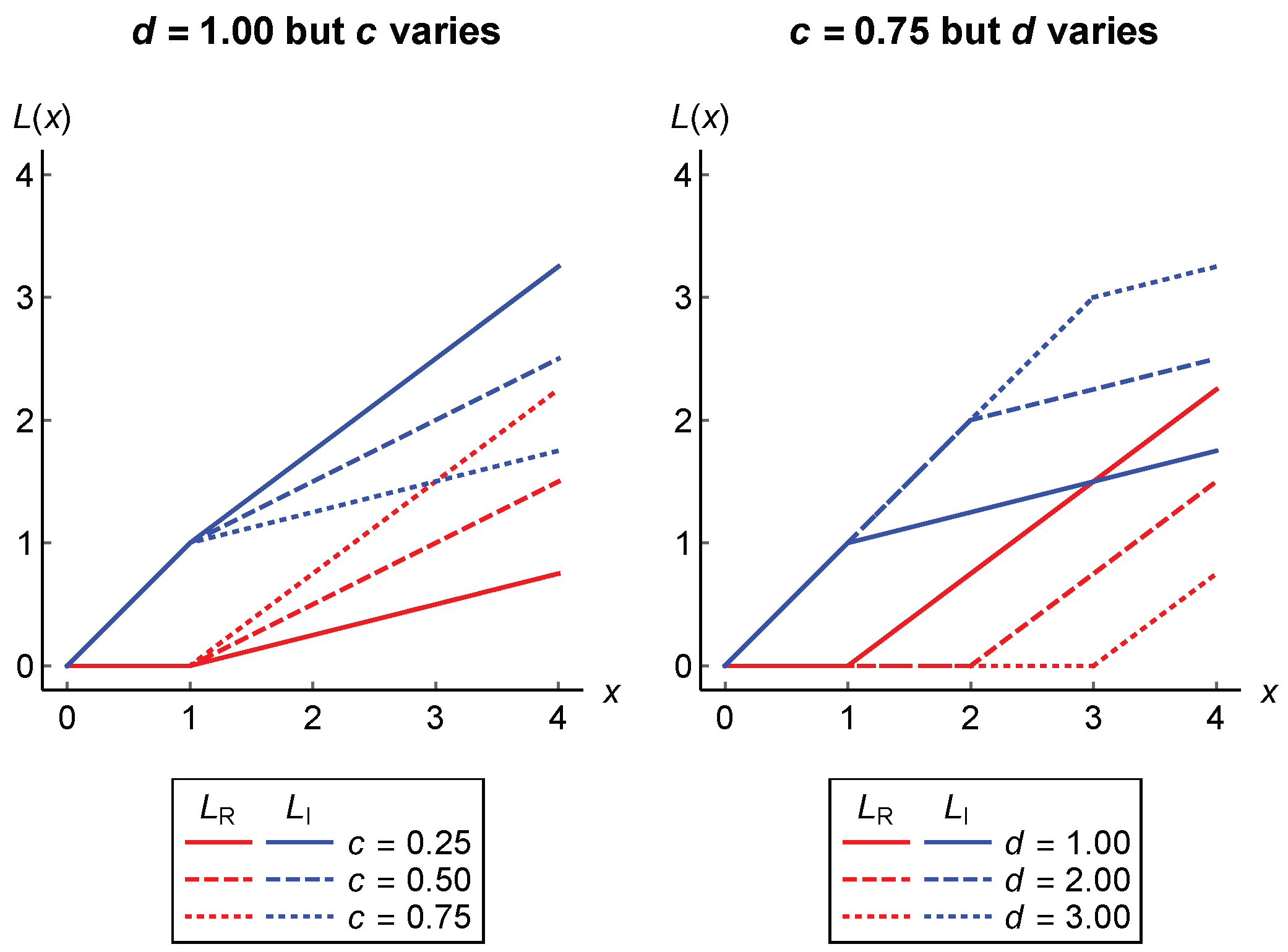
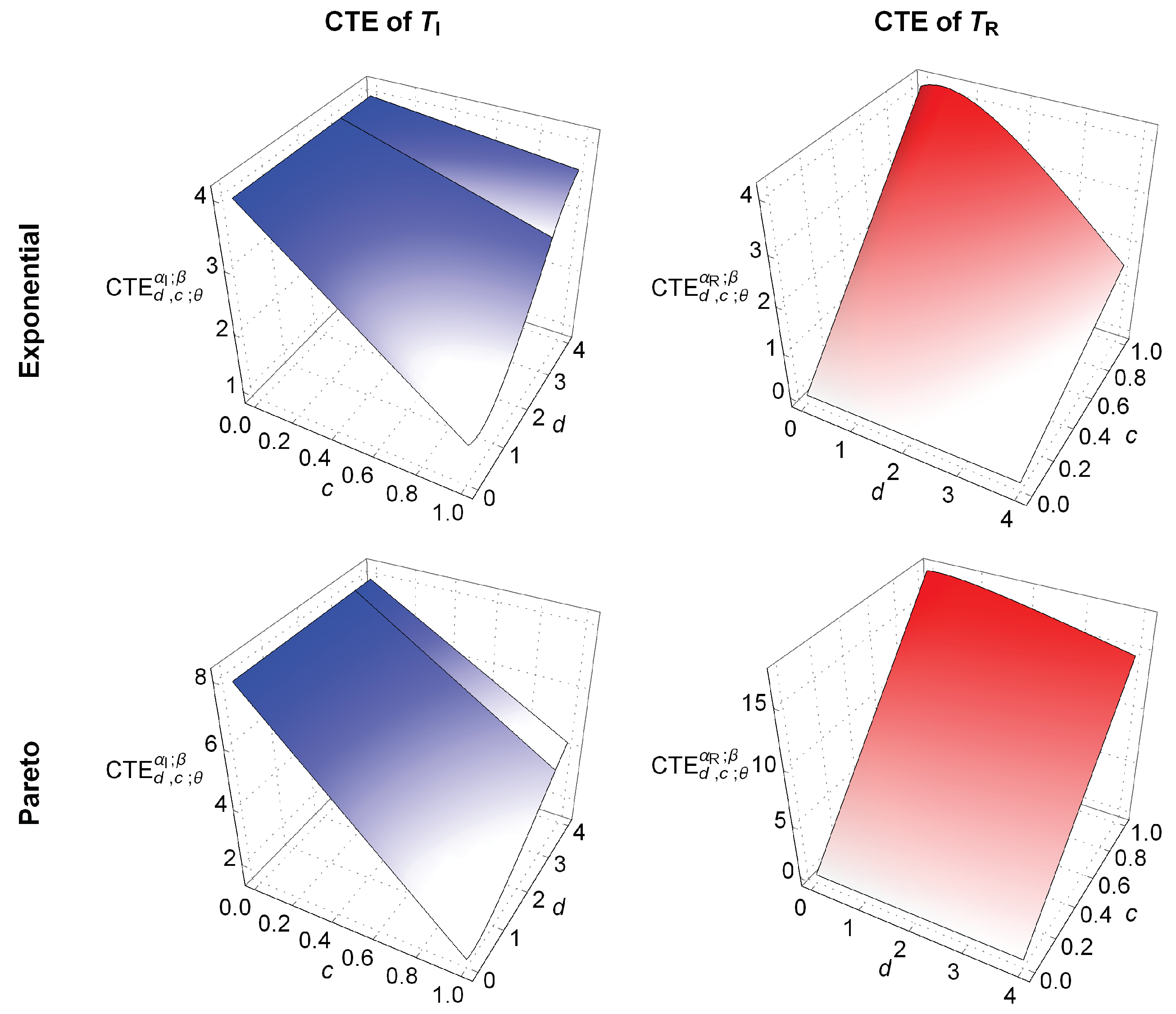
The influence of the retention limit d and the retention level c on the values of the above CTEs is depicted in Figure 3. It may be observed that as the value of d increases, the value of ${\mathrm{CTE}}_{d,c;\theta }^{{\alpha }_{\mathrm{I}};\beta }(T_{\mathrm{I}})$ initially decreases and, then, increases after attaining its minimum. Meanwhile, the increase of ${\mathrm{CTE}}_{d,c;\theta }^{{\alpha }_{\mathrm{R}};\beta }(T_{\mathrm{R}})$ initially occurs and is then followed by the decrease after reaching a peak. 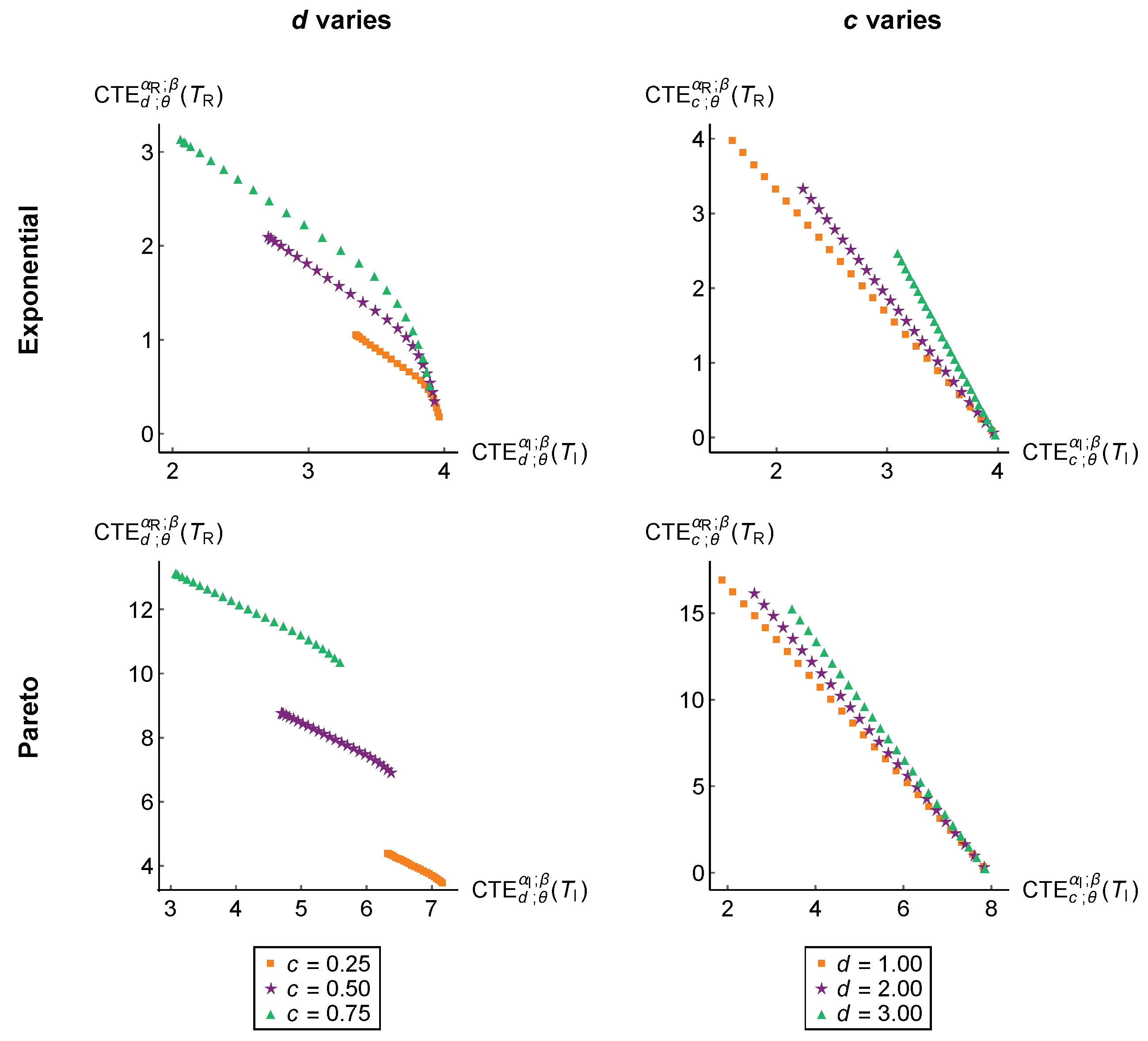Furthermore, as the value of c increases, the value of ${\mathrm{CTE}}_{d,c;\theta }^{{\alpha }_{\mathrm{I}};\beta }(T_{\mathrm{I}})$ decreases linearly whilst the value of ${\mathrm{CTE}}_{d,c;\theta }^{{\alpha }_{\mathrm{R}};\beta }(T_{\mathrm{R}})$ increases linearly. This illustration indicates that ${\mathrm{CTE}}_{d,c;\theta }^{{\alpha }_{\mathrm{I}};\beta }(T_{\mathrm{I}})$ is shown to be inversely proportional to ${\mathrm{CTE}}_{d,c;\theta }^{{\alpha }_{\mathrm{R}};\beta }(T_{\mathrm{R}})$, which means that the CTE of the total loss for one party decreases as the CTE of the total loss for another party increases. This relationship may noticeably be observed from the other visualizations provided in Figure 4 and Figure 5.

3.2. Optimization from Joint Perspective of Insurer and Reinsurer

We have assumed that the CTE is utilized by both the insurer and the reinsurer to measure their own total losses. From the perspective of the insurer, the insurer desires to buy the combined stop-loss and quota-share reinsurance whose parameters denoting retentions are solutions to the optimization problem

$$\underset{(d,c)\in \mathfrak{D}}{min}{\mathrm{CTE}}_{d,c;\theta }^{{\alpha }_{\mathrm{I}};\beta }(T_{\mathrm{I}}).$$

(16)

Meanwhile, from the reinsurer’s viewpoint, the reinsurer prefers to offer the combined stop-loss and quota-share reinsurance whose retentions are solutions to the optimization problem

$$\underset{(d,c)\in \mathfrak{D}}{min}{\mathrm{CTE}}_{d,c;\theta }^{{\alpha }_{\mathrm{R}};\beta }(T_{\mathrm{R}}).$$

(17)

However, the optimal retentions of the combined stop-loss and quota-share reinsurance for one party are different from those for another party and is not optimal from its perspective. We, therefore, do not consider finding the minimizers of the CTEs of the insurer’s total loss and the reinsurer’s total loss by solving Problems (16) and (17) separately. Since the increase of the total loss faced by one party causes the decrease of the total loss covered by another party, we, in this paper, aim at carrying out the following optimization problem:

$$\underset{(d,c)\in \mathfrak{D}}{min}{\Psi }_{d,c;\theta }^{{\alpha }_{\mathrm{I}},{\alpha }_{\mathrm{R}};\beta ,\omega }(T_{\mathrm{I}},T_{\mathrm{R}}),$$

(18)

where

$${\Psi }_{d,c;\theta }^{{\alpha }_{\mathrm{I}},{\alpha }_{\mathrm{R}};\beta ,\omega }(T_{\mathrm{I}},T_{\mathrm{R}})=\omega {\mathrm{CTE}}_{d,c;\theta }^{{\alpha }_{\mathrm{I}};\beta }(T_{\mathrm{I}})+(1-\omega ){\mathrm{CTE}}_{d,c;\theta }^{{\alpha }_{\mathrm{R}};\beta }(T_{\mathrm{R}})$$

(19)

for a specified weighting factor $\omega \in [0,1]$. Minimizing such a convex combination of ${\mathrm{CTE}}_{d,c;\theta }^{{\alpha }_{\mathrm{I}};\beta }(T_{\mathrm{I}})$ and ${\mathrm{CTE}}_{d,c;\theta }^{{\alpha }_{\mathrm{R}};\beta }(T_{\mathrm{R}})$ considered as the objective function is expected to produce optimal retentions that are acceptable to both parties. Note that when $\omega$ is set to be one, we actually do the optimization from the point of view of the insurer. Meanwhile, the optimization from the reinsurer’s perspective is for $\omega =0$. This means that Problems (16) and (17) are special cases of Problem (18).

For simplicity, we introduce the following additional notations:

$$\begin{array}{cc}\hfill {\omega }^{*}& =\frac{\omega }{2\omega -1},\hfill \\ \hfill {\beta }^{*}& =\frac{1}{1+\beta },\hfill \\ \hfill {\beta }_{\omega }^{*}& =\frac{{\omega }^{*}-1}{\frac{{\omega }^{*}}{{\alpha }_{\mathrm{I}}}-\frac{1}{{\beta }^{*}}},\hfill \\ \hfill G_{\theta }^{\beta }(d)& =d+\frac{1}{{\beta }^{*}}{K}_{\theta }(d),\hfill \\ \hfill H_{\theta }^{{\alpha }_{\mathrm{I}},{\alpha }_{\mathrm{R}};\omega }(d)& ={\omega }^{*}\left\{d\vee {\mathrm{VaR}}_{\theta }^{{\alpha }_{\mathrm{I}}}(X)+\frac{1}{{\alpha }_{\mathrm{I}}}{K}_{\theta }\left[d\vee {\mathrm{VaR}}_{\theta }^{{\alpha }_{\mathrm{I}}}(X)\right]\right\}-({\omega }^{*}-1){\mathrm{CTE}}_{\theta }^{{\alpha }_{\mathrm{R}}}(X).\hfill \end{array}$$

By substituting the CTEs of the total losses for both the insurer and the reinsurer, given in Equations (14) and (15), to Equation (19), we may formulate the objective function in terms of the above notations as follows:

$${\Psi }_{d,c;\theta }^{{\alpha }_{\mathrm{I}},{\alpha }_{\mathrm{R}};\beta ,\omega }(T_{\mathrm{I}},T_{\mathrm{R}})=\omega {\mathrm{CTE}}_{\theta }^{{\alpha }_{\mathrm{I}}}(X)+(2\omega -1)c\left[G_{\theta }^{\beta }(d)-H_{\theta }^{{\alpha }_{\mathrm{I}},{\alpha }_{\mathrm{R}};\omega }(d)\right].$$

The pair of optimal retentions $(d_{\theta },c_{\theta })\in \mathfrak{D}$ is summarized in the following theorems whose proofs are explained in Appendix A. Since the value of d depends on both ${\mathrm{VaR}}_{\theta }^{{\alpha }_{\mathrm{I}}}(X)$ and ${\mathrm{VaR}}_{\theta }^{{\alpha }_{\mathrm{R}}}(X)$, and hence on both the significance levels of ${\alpha }_{\mathrm{I}}$ and ${\alpha }_{\mathrm{R}}$, the theorems are provided separately under the condition (1) ${\alpha }_{\mathrm{I}}\le {\alpha }_{\mathrm{R}}$ or (2) ${\alpha }_{\mathrm{R}}<{\alpha }_{\mathrm{I}}$.

Theorem 1.

Under the condition ${\alpha }_{\mathrm{I}}\le {\alpha }_{\mathrm{R}}$, the optimal retentions as the solutions to Problem (18) are derived for $\omega >\frac{1}{2}$ with the following values:

1.

$(d_{\theta },c_{\theta })=\left({\mathrm{VaR}}_{\theta }^{{\beta }^{*}}(X),1\right)$ when ${\alpha }_{\mathrm{R}}<{\beta }^{*}<S_{X;\theta }(0)$ and $G_{\theta }^{\beta }(d_{\theta })<H_{\theta }^{{\alpha }_{\mathrm{I}},{\alpha }_{\mathrm{R}};\omega }(d_{\theta })$;

2.

$(d_{\theta },c_{\theta })=\left({\mathrm{VaR}}_{\theta }^{{\beta }^{*}}(X),u\right)$ for any constant $u\in (0,1]$ when ${\alpha }_{\mathrm{R}}<{\beta }^{*}<S_{X;\theta }(0)$ and $G_{\theta }^{\beta }(d_{\theta })=H_{\theta }^{{\alpha }_{\mathrm{I}},{\alpha }_{\mathrm{R}};\omega }(d_{\theta })$;

3.

$(d_{\theta },c_{\theta })=\left({\mathrm{VaR}}_{\theta }^{{\alpha }_{\mathrm{R}}}(X),1\right)$ when ${\beta }^{*}\le {\alpha }_{\mathrm{R}}$ and $G_{\theta }^{\beta }(d_{\theta })<H_{\theta }^{{\alpha }_{\mathrm{I}},{\alpha }_{\mathrm{R}};\omega }(d_{\theta })$;

4.

$(d_{\theta },c_{\theta })=\left({\mathrm{VaR}}_{\theta }^{{\alpha }_{\mathrm{R}}}(X),u\right)$ for any constant $u\in (0,1]$ when ${\beta }^{*}\le {\alpha }_{\mathrm{R}}$ and $G_{\theta }^{\beta }(d_{\theta })=H_{\theta }^{{\alpha }_{\mathrm{I}},{\alpha }_{\mathrm{R}};\omega }(d_{\theta })$.

Theorem 2.

Under the condition ${\alpha }_{\mathrm{R}}<{\alpha }_{\mathrm{I}}$, the optimal retentions as the solutions to Problem (18) are derived for $\omega >\frac{1}{2}$ with the following values:

1.

$(d_{\theta },c_{\theta })=\left({\mathrm{VaR}}_{\theta }^{{\beta }^{*}}(X),1\right)$ when ${\beta }_{\omega }^{*}\le {\alpha }_{\mathrm{R}}$, ${\alpha }_{\mathrm{I}}<{\beta }^{*}<S_{X;\theta }(0)$, and $G_{\theta }^{\beta }(d_{\theta })<H_{\theta }^{{\alpha }_{\mathrm{I}},{\alpha }_{\mathrm{R}};\omega }(d_{\theta })$;

2.

$(d_{\theta },c_{\theta })=\left({\mathrm{VaR}}_{\theta }^{{\beta }^{*}}(X),u\right)$ for any constant $u\in (0,1]$ when ${\beta }_{\omega }^{*}\le {\alpha }_{\mathrm{R}}$, ${\alpha }_{\mathrm{I}}<{\beta }^{*}<S_{X;\theta }(0)$, and $G_{\theta }^{\beta }(d_{\theta })=H_{\theta }^{{\alpha }_{\mathrm{I}},{\alpha }_{\mathrm{R}};\omega }(d_{\theta })$;

3.

$(d_{\theta },c_{\theta })=\left({\mathrm{VaR}}_{\theta }^{{\alpha }_{\mathrm{R}}}(X),1\right)$ when ${\beta }^{*}<{\omega }^{*}{\beta }^{*}<{\alpha }_{\mathrm{I}}$ and $G_{\theta }^{\beta }(d_{\theta })<H_{\theta }^{{\alpha }_{\mathrm{I}},{\alpha }_{\mathrm{R}};\omega }(d_{\theta })$;

4.

$(d_{\theta },c_{\theta })=\left({\mathrm{VaR}}_{\theta }^{{\alpha }_{\mathrm{R}}}(X),u\right)$ for any constant $u\in (0,1]$ when ${\beta }^{*}<{\omega }^{*}{\beta }^{*}<{\alpha }_{\mathrm{I}}$ and $G_{\theta }^{\beta }(d_{\theta })=H_{\theta }^{{\alpha }_{\mathrm{I}},{\alpha }_{\mathrm{R}};\omega }(d_{\theta })$.

Theorems 1 and 2 above tell us important results of optimizing the combined stop-loss and quota-share reinsurance as follows. First, when the loading factor $\beta$ is chosen such that the value of ${\beta }^{*}$ is higher than the significance levels used by both the insurer and the reinsurer, the optimal retention limit $d_{\theta }$ may be found to be equal to the VaR of the initial loss at the probability level of ${\beta }^{*}$. The value of this optimal retention limit is lower than both ${\mathrm{VaR}}_{\theta }^{{\alpha }_{\mathrm{I}}}(X)$ and ${\mathrm{VaR}}_{\theta }^{{\alpha }_{\mathrm{R}}}(X)$. Meanwhile, if ${\beta }^{*}$ is too small and, as a result, ${\mathrm{VaR}}_{\theta }^{{\beta }^{*}}(X)$ is too large, then we may set the VaR of X at the ${\alpha }_{\mathrm{R}}$ level as the optimal retention limit. This is because the possible value of d is bounded above by this VaR. The optimality of the retention limit is achieved when the other criteria involving the weighting factor $\omega$ and the parameter $\theta$ of the distribution of X are satisfied.

Second, the optimal retention level $c_{\theta }$ is determined based on the condition whether the values of $G_{\theta }^{\beta }$ and $H_{\theta }^{{\alpha }_{\mathrm{I}},{\alpha }_{\mathrm{R}};\omega }$ evaluated at the retention limit $d_{\theta }$ are equal. If the former is lower than the latter, we obtain $c_{\theta }=1$, which means that the objective function ${\Psi }_{d,c;\theta }^{{\alpha }_{\mathrm{I}},{\alpha }_{\mathrm{R}};\beta ,\omega }$ employed in the optimization problem attains its minimum at the unique point $(d_{\theta },c_{\theta })$. Meanwhile, the equality $G_{\theta }^{\beta }(d_{\theta })=H_{\theta }^{{\alpha }_{\mathrm{I}},{\alpha }_{\mathrm{R}};\omega }(d_{\theta })$ makes the minimum value of ${\Psi }_{d,c;\theta }^{{\alpha }_{\mathrm{I}},{\alpha }_{\mathrm{R}};\beta ,\omega }$ attained at each point $(d,c)\in \left\{d_{\theta }\right\}\times (0,1]$. This situation allows us to choose any number in $(0,1]$ as the optimal retention level $c_{\theta }$.

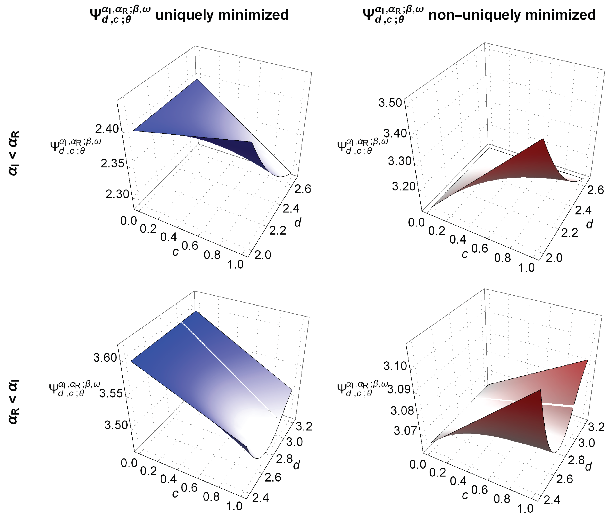
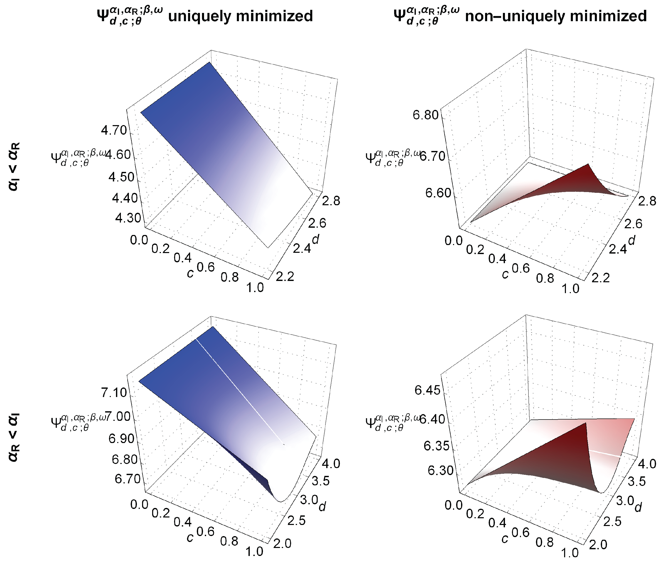
In Figure 6 and Figure 7, we illustrate the surfaces of ${\Psi }_{d,c;\theta }^{{\alpha }_{\mathrm{I}},{\alpha }_{\mathrm{R}};\beta ,\omega }$ when the initial loss X is assumed to follow an exponential distribution $\mathcal{E}(\theta )$ and a Pareto distribution $\mathcal{P}(\theta )$, respectively. Such surfaces are provided according to the results in Parts 3 and 4 of Theorem 1 and Parts 1 and 2 of Theorem 2. These illustrations are respectively denoted into four cases as follows.

• Case A:${\alpha }_{\mathrm{I}}\le {\alpha }_{\mathrm{R}}$ where ${\Psi }_{d,c;\theta }^{{\alpha }_{\mathrm{I}},{\alpha }_{\mathrm{R}};\beta ,\omega }$ is uniquely minimized (see row 1 and column 1).
• Case B:${\alpha }_{\mathrm{I}}\le {\alpha }_{\mathrm{R}}$ where ${\Psi }_{d,c;\theta }^{{\alpha }_{\mathrm{I}},{\alpha }_{\mathrm{R}};\beta ,\omega }$ is non-uniquely minimized (see row 1 and column 2).
• Case C:${\alpha }_{\mathrm{R}}<{\alpha }_{\mathrm{I}}$ where ${\Psi }_{d,c;\theta }^{{\alpha }_{\mathrm{I}},{\alpha }_{\mathrm{R}};\beta ,\omega }$ is uniquely minimized (see row 2 and column 1).
• Case D:${\alpha }_{\mathrm{R}}<{\alpha }_{\mathrm{I}}$ where ${\Psi }_{d,c;\theta }^{{\alpha }_{\mathrm{I}},{\alpha }_{\mathrm{R}};\beta ,\omega }$ is non-uniquely minimized (see row 2 and column 2).

When $X\sim \mathcal{E}(\theta )$, the pair of optimal retentions for the combined stop-loss and quota-share reinsurance are given by

$$(d_{\theta },c_{\theta })=\left\{\begin{array}{cc}\left(\frac{1}{\theta }(-ln{\alpha }_{\mathrm{R}}),1\right),\hfill & \mathrm{for}\mathrm{Case}\mathrm{A},\hfill \\ \left(\frac{1}{\theta }(-ln{\alpha }_{\mathrm{R}}),u\right),u\in (0,1],\hfill & \mathrm{for}\mathrm{Case}\mathrm{B},\hfill \\ \left(\frac{1}{\theta }(-ln{\beta }^{*}),1\right),\hfill & \mathrm{for}\mathrm{Case}\mathrm{C},\hfill \\ \left(\frac{1}{\theta }(-ln{\beta }^{*}),u\right),u\in (0,1],\hfill & \mathrm{for}\mathrm{Case}\mathrm{D}.\hfill \end{array}\right.$$

(20)

Meanwhile, below we express the pair of optimal retentions when X follows $\mathcal{P}(\theta )$:

$$(d_{\theta },c_{\theta })=\left\{\begin{array}{cc}\left({\alpha }_{\mathrm{R}}^{-1/\theta }-1,1\right),\hfill & \mathrm{for}\mathrm{Case}\mathrm{A},\hfill \\ \left({\alpha }_{\mathrm{R}}^{-1/\theta }-1,u\right),u\in (0,1],\hfill & \mathrm{for}\mathrm{Case}\mathrm{B},\hfill \\ \left({({\beta }^{*})}^{-1/\theta }-1,1\right),\hfill & \mathrm{for}\mathrm{Case}\mathrm{C},\hfill \\ \left({({\beta }^{*})}^{-1/\theta }-1,u\right),u\in (0,1],\hfill & \mathrm{for}\mathrm{Case}\mathrm{D}.\hfill \end{array}\right.$$

(21)

4. Estimation for Optimal Retentions with Numerical Examples

We see that the optimal retentions $d_{\theta }$ and $c_{\theta }$ for the combined stop-loss and quota-share reinsurance, which have been derived in Section 3, depend on an unknown parameter, $\theta$, of the loss distribution and may be viewed as functions of $\theta$. Their explicit expressions have been found when, for instance, the loss X is assumed to follow an exponential distribution $\mathcal{E}(\theta )$, $\theta \in (0,\infty )$, or a Pareto distribution $\mathcal{P}(\theta )$, $\theta \in (1,\infty )$. In this section, we now consider finding the estimate for $\theta$, $\widehat{\theta }$. When the parameter $\theta$ in the optimal retentions $d_{\theta }$ and $c_{\theta }$ is replaced by $\widehat{\theta }$, we then obtain a pair $\left({\widehat{d}}_{\widehat{\theta }},{\widehat{c}}_{\widehat{\theta }}\right)$ of the estimated optimal retentions.

Suppose that $\{X_1,X_2,\dots ,X_n\}$ is a sample of size n randomly drawn from X. From this random sample, the estimate $\widehat{\theta }$ may be found by employing the well-known maximum likelihood method. If $x_1,x_2,\dots ,x_n$ denote the realizations of $X_1,X_2,\dots ,X_n$, respectively, such $\widehat{\theta }$ is a solution to the optimization problem

$$\underset{\theta \in \Omega }{max}\ell (\theta ;x_1,x_2,\dots ,x_n),$$

where $\ell (\theta ;x_1,x_2,\dots ,x_n)$ is the log-likelihood function evaluated at $x_1,x_2,\dots ,x_n$. Such an objective function is given by $\ell (\theta ;x_1,x_2,\dots ,x_n)={\sum }_{i=1}^{n}ln{f}_{X;\theta }(x_i)$, where $f_{X;\theta }$ is the probability function of X.

When the random sample is drawn from the exponential distribution $\mathcal{E}(\theta )$, a statistic $\widehat{\theta }=1/\overline{X}$ may be found to be an estimate for $\theta$, where $\overline{X}={\sum }_{i=1}^n{X}_i/n$ is the mean of the random sample. By substituting such $\widehat{\theta }$ to the optimal retentions given in Equation (20), we derive their estimate as follows:

$${\widehat{d}}_{\widehat{\theta }}=\frac{1}{\widehat{\theta }}(-ln\delta )=\overline{X}(-ln\delta ),$$

where $\delta$ represents ${\alpha }_{\mathrm{R}}$ or ${\beta }^{*}$, whilst ${\widehat{c}}_{\widehat{\theta }}$ is a constant in $(0,1]$. By taking their expected value, we find that

$$\mathbb{E}\left({\widehat{d}}_{\widehat{\theta }}\right)=\mathbb{E}\left(\overline{X}\right)(-ln\delta )=\frac{1}{\theta }(-ln\delta )=d_{\theta }$$

and $\mathbb{E}\left({\widehat{c}}_{\widehat{\theta }}\right)=c_{\theta }$. This shows that when the initial loss is exponentially distributed, the pair $\left({\widehat{d}}_{\widehat{\theta }},{\widehat{c}}_{\widehat{\theta }}\right)$ is an unbiased estimate for the pair $(d_{\theta },c_{\theta })$ of the optimal retentions for the combined stop-loss and quota-share reinsurance.

On the other hand, if the random sample from $\mathcal{P}(\theta )$ is taken into consideration, we derive the following statistic for estimating $\theta$:

$$\widehat{\theta }=\frac{1}{{\sum }_{i=1}^{n}ln(1+X_i)/n}.$$

Consequently, based on Equation (21), the estimate for the retention limit is given by

$${\widehat{d}}_{\widehat{\theta }}={\delta }^{-1/\widehat{\theta }}-1={\delta }^{-{\sum }_{i=1}^{n}ln(1+X_i)/n}-1,$$

where $\delta \in \{{\alpha }_{\mathrm{R}},{\beta }^{*}\}$, whilst ${\widehat{c}}_{\widehat{\theta }}$ is a constant in $(0,1]$. It is easy to verify that $ln(1+X_i)\sim \mathcal{E}(\theta )$, for all $i\in \{1,2,\dots ,n\}$, and, hence, the statistic $Y={\sum }_{i=1}^{n}ln(1+X_i)/n$ has a gamma distribution $\mathcal{G}(n,n\theta )$ with probability function $f_{Y;n,\theta }(y)={(n\theta )}^n{y}^{n-1}{\mathrm{e}}^{-n\theta y}/(n-1)!$, $y>0$. As a result, $\mathbb{E}\left({\widehat{c}}_{\widehat{\theta }}\right)=c_{\theta }$ whilst

$$\mathbb{E}\left({\widehat{d}}_{\widehat{\theta }}\right)=\mathbb{E}\left({\delta }^{-Y}\right)-1={\left(1+\frac{ln\delta }{n\theta }\right)}^{-n}-1$$

that differs from ${\delta }^{-1/\theta }-1$, for all $n\in \mathbb{N}$. If its limit is taken as $n\to \infty$, we then obtain

$$\underset{n\to \infty }{lim}\mathbb{E}\left({\widehat{d}}_{\widehat{\theta }}\right)={\mathrm{e}}^{-(ln\delta )/\theta }-1={\delta }^{-1/\theta }-1=d_{\theta }.$$

This indicates that the pair $\left({\widehat{d}}_{\widehat{\theta }},{\widehat{c}}_{\widehat{\theta }}\right)$ is a biased estimate for the pair $(d_{\theta },c_{\theta })$ if the initial loss follows the Pareto distribution. However, such an estimate is expected to be close to the actual value of the optimal retention when the sample size n is large enough.

To investigate the impact of the sample size n on the estimated parameter $\widehat{\theta }$ as well as on the pair $\left({\widehat{d}}_{\widehat{\theta }},{\widehat{c}}_{\widehat{\theta }}\right)$ of the estimated optimal retentions and the corresponding value of the objective function minimized at such $\left({\widehat{d}}_{\widehat{\theta }},{\widehat{c}}_{\widehat{\theta }}\right)$, we provide numerical examples. Specifically, we conducted numerical simulations for various values of $\theta$ and n through a Monte Carlo approach with $m=10,000$ runs. The accuracy of those estimates is assessed by using root-mean-square error (RMSE) defined by

$$\mathrm{RMSE}(\vartheta )=\sqrt{{\sum }_{j=1}^m\frac{{({\widehat{\vartheta }}_j-\vartheta )}^2}{m}},$$

where $\vartheta$ denotes an actual value of the parameter $\theta$, the optimal retention, or the minimized objective function whilst ${\widehat{\vartheta }}_j$ is its estimate computed at the jth run, for all $j\in \{1,2,\dots ,m\}$.

The results of the numerical simulations are provided in

Table 1. The estimated optimal retentions for the combined stop-loss and quota-share reinsurance and the corresponding value of the minimized objective function when the initial loss follows an exponential or Pareto distribution. The RMSE of each estimate is given in parenthesis.

Case	Exponential						Pareto
	$\mathit{\theta }$	$\mathit{n}$	$\widehat{\mathit{\theta }}$	${\widehat{\mathit{d}}}_{\widehat{\mathit{\theta }}}$	${\widehat{\mathit{c}}}_{\widehat{\mathit{\theta }}}$	${\widehat{\mathbf{\Psi }}}_{{\widehat{\mathit{d}}}_{\widehat{\mathit{\theta }}}\mathbf{,}{\widehat{\mathit{c}}}_{\widehat{\mathit{\theta }}}\mathbf{;}\widehat{\mathit{\theta }}}^{{\mathit{\alpha }}_{\mathbf{I}}\mathbf{,}{\mathit{\alpha }}_{\mathbf{R}}\mathbf{;}\mathit{\beta }\mathbf{,}\mathit{\omega }}$	$\mathit{\theta }$	$\mathit{n}$	$\widehat{\mathit{\theta }}$	${\widehat{\mathit{d}}}_{\widehat{\mathit{\theta }}}$	${\widehat{\mathit{c}}}_{\widehat{\mathit{\theta }}}$	${\widehat{\mathbf{\Psi }}}_{{\widehat{\mathit{d}}}_{\widehat{\mathit{\theta }}}\mathbf{,}{\widehat{\mathit{c}}}_{\widehat{\mathit{\theta }}}\mathbf{;}\widehat{\mathit{\theta }}}^{{\mathit{\alpha }}_{\mathbf{I}}\mathbf{,}{\mathit{\alpha }}_{\mathbf{R}}\mathbf{;}\mathit{\beta }\mathbf{,}\mathit{\omega }}$
A	2.00	10	2.23 (0.84)	1.33 (0.43)	1	1.17 (0.11)	3.00	10	3.27 (1.23)	1.61 (0.95)	1	1.70 (0.23)
		100	2.02 (0.21)	1.33 (0.13)	1	1.15 (0.02)		100	3.02 (0.32)	1.44 (0.23)	1	1.70 (0.03)
		1000	2.00 (0.06)	1.33 (0.04)	1	1.15 (0.00)		1000	3.00 (0.10)	1.43 (0.07)	1	1.70 (0.01)
	1.00	10	1.10 (0.40)	2.68 (0.85)	1	2.34 (0.22)	2.00	10	2.18 (0.82)	3.56 (3.42)	1	4.19 (0.99)
		100	1.01 (0.10)	2.66 (0.26)	1	2.30 (0.03)		100	2.01 (0.22)	2.84 (0.56)	1	4.30 (0.06)
		1000	1.00 (0.03)	2.66 (0.08)	1	2.29 (0.01)		1000	2.00 (0.07)	2.79 (0.17)	1	4.29 (0.02)
	0.50	10	0.56 (0.20)	5.32 (1.68)	1	4.69 (0.44)	1.50	10	1.63 (0.63)	7.66 (13.60)	1	10.53 (4.68)
		100	0.51 (0.05)	5.31 (0.53)	1	4.60 (0.06)		100	1.51 (0.17)	5.06 (1.24)	1	11.13 (0.13)
		1000	0.50 (0.02)	5.32 (0.17)	1	4.58 (0.02)		1000	1.50 (0.05)	4.90 (0.36)	1	11.11 (0.03)
B	2.00	10	2.23 (0.84)	1.33 (0.43)	(0,1]	1.67 (0.27)	3.00	10	3.27 (1.23)	1.61 (0.95)	(0,1]	2.61 (0.38)
		100	2.02 (0.21)	1.33 (0.13)	(0,1]	1.57 (0.05)		100	3.02 (0.32)	1.44 (0.23)	(0,1]	2.49 (0.08)
		1000	2.00 (0.06)	1.33 (0.04)	(0,1]	1.56 (0.01)		1000	3.00 (0.10)	1.43 (0.07)	(0,1]	2.47 (0.02)
	1.00	10	1.10 (0.40)	2.68 (0.85)	(0,1]	3.33 (0.54)	2.00	10	2.18 (0.82)	3.56 (3.42)	(0,1]	6.76 (0.91)
		100	1.01 (0.10)	2.66 (0.26)	(0,1]	3.14 (0.09)		100	2.01 (0.22)	2.84 (0.56)	(0,1]	6.56 (0.18)
		1000	1.00 (0.03)	2.66 (0.08)	(0,1]	3.11 (0.02)		1000	2.00 (0.07)	2.79 (0.17)	(0,1]	6.52 (0.05)
	0.50	10	0.56 (0.20)	5.32 (1.68)	(0,1]	6.68 (1.11)	1.50	10	1.63 (0.63)	7.66 (13.60)	(0,1]	17.97 (2.52)
		100	0.51 (0.05)	5.31 (0.53)	(0,1]	6.28 (0.17)		100	1.51 (0.17)	5.06 (1.24)	(0,1]	17.73 (0.39)
		1000	0.50 (0.02)	5.32 (0.17)	(0,1]	6.23 (0.04)		1000	1.50 (0.05)	4.90 (0.36)	(0,1]	17.64 (0.11)
C	2.00	10	2.23 (0.84)	1.39 (0.44)	1	1.85 (0.24)	3.00	10	3.27 (1.23)	1.73 (1.05)	1	2.75 (0.27)
		100	2.02 (0.21)	1.39 (0.14)	1	1.75 (0.02)		100	3.02 (0.32)	1.54 (0.25)	1	2.63 (0.04)
		1000	2.00 (0.06)	1.39 (0.04)	1	1.74 (0.00)		1000	3.00 (0.10)	1.52 (0.08)	1	2.61 (0.00)
	1.00	10	1.10 (0.40)	2.79 (0.89)	1	3.68 (0.44)	2.00	10	2.18 (0.82)	3.90 (3.95)	1	6.95 (0.59)
		100	1.01 (0.10)	2.77 (0.28)	1	3.50 (0.04)		100	2.01 (0.22)	3.07 (0.62)	1	6.71 (0.09)
		1000	1.00 (0.03)	2.77 (0.09)	1	3.47 (0.01)		1000	2.00 (0.07)	3.01 (0.19)	1	6.66 (0.01)
	0.50	10	0.56 (0.20)	5.55 (1.75)	1	7.37 (0.91)	1.50	10	1.63 (0.63)	8.67 (16.88)	1	17.93 (1.65)
		100	0.51 (0.05)	5.54 (0.55)	1	6.99 (0.09)		100	1.51 (0.17)	5.55 (1.40)	1	17.57 (0.19)
		1000	0.50 (0.02)	5.55 (0.17)	1	6.94 (0.01)		1000	1.50 (0.05)	5.37 (0.41)	1	17.46 (0.03)
D	2.00	10	2.23 (0.84)	1.39 (0.44)	(0,1]	1.60 (0.16)	3.00	10	3.27 (1.23)	1.73 (1.05)	(0,1]	2.48 (0.21)
		100	2.02 (0.21)	1.39 (0.14)	(0,1]	1.54 (0.02)		100	3.02 (0.32)	1.54 (0.25)	(0,1]	2.42 (0.03)
		1000	2.00 (0.06)	1.39 (0.04)	(0,1]	1.53 (0.00)		1000	3.00 (0.10)	1.52 (0.08)	(0,1]	2.40 (0.00)
	1.00	10	1.10 (0.40)	2.79 (0.89)	(0,1]	3.19 (0.29)	2.00	10	2.18 (0.82)	3.90 (3.95)	(0,1]	6.39 (0.67)
		100	1.01 (0.10)	2.77 (0.28)	(0,1]	3.08 (0.03)		100	2.01 (0.22)	3.07 (0.62)	(0,1]	6.31 (0.06)
		1000	1.00 (0.03)	2.77 (0.09)	(0,1]	3.07 (0.00)		1000	2.00 (0.07)	3.01 (0.19)	(0,1]	6.28 (0.01)
	0.50	10	0.56 (0.20)	5.55 (1.75)	(0,1]	6.39 (0.61)	1.50	10	1.63 (0.63)	8.67 (16.88)	(0,1]	16.86 (2.95)
		100	0.51 (0.05)	5.54 (0.55)	(0,1]	6.16 (0.06)		100	1.51 (0.17)	5.55 (1.40)	(0,1]	16.91 (0.13)
		1000	0.50 (0.02)	5.55 (0.17)	(0,1]	6.13 (0.01)		1000	1.50 (0.05)	5.37 (0.41)	(0,1]	16.84 (0.02)

with four panels based on four cases (A, B, C, and D) stated at the end of Section 3. Each row at each panel compares the exponential and Pareto random losses with equal mean. We find that as the sample size increases, the estimates for the parameter, the optimal retention, and the minimized objective function tend to be more accurate with small RMSE. When the actual parameter decreases indicating that the mean of the initial loss increases, the RMSE of the parameter estimate decreases. However, the accuracy of the estimates for the optimal retention and the minimized objective function appears to decrease due to the increase of their RMSE. Furthermore, the Pareto distribution produces less accurate estimates than the exponential loss. This is in line with the theoretical explanation discussed above. The accuracy is extremely poor when the actual parameter of the Pareto distribution is close to 1. This is because its tail is heavier with evidence of having extreme simulated losses.

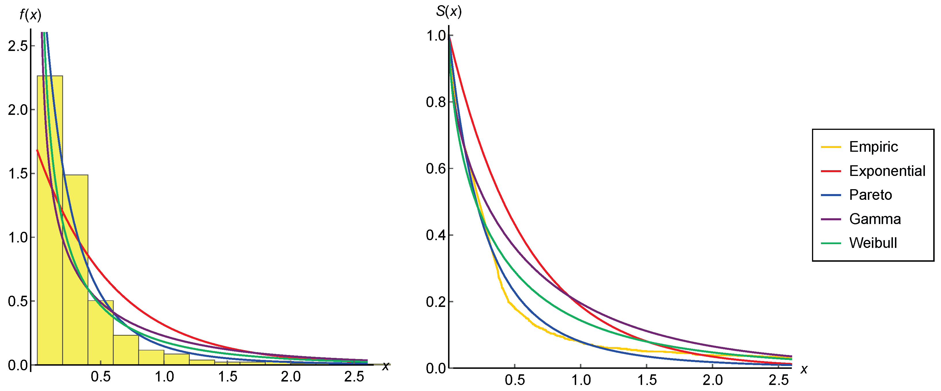
To illustrate a more complete overview of our theoretical findings, we employ a real data set consisting of total economic losses or claims (in ten thousand dollars) from $n=1340$ claimants. Such claims arise from automobile bodily injury insurance coverages; see Frees (2010). Statistics, including four (central) moments of these empirical data, are given in

Table 2. The parameter estimates for several parametric distributions based on the empirical claim data along with the comparison of the estimates for their four (central) moments.

Distribution	Parameter	Log-Likelihood	AIC	Mean	Variance	Skewness	Kurtosis
Empiric				0.60	10.98	25.69	794.67
Exponential $(\theta )$	1.68	$-645.06$	1292.12	0.60	0.35	2.00	9.00
Pareto $(\theta )$	3.65	$-94.28$	190.55	0.38	0.32	9.62	-
Gamma $({\theta }_1,{\theta }_2)$	$(0.52,0.87)$	$-383.76$	771.52	0.60	0.69	2.79	14.65
Weibull $({\theta }_1,{\theta }_2)$	$(0.65,0.36)$	$-208.65$	421.30	0.49	0.62	3.98	30.32

. An extremely high empirical kurtosis, that is found to be equal to 794.67, leads us to employ a heavy-tailed loss model for such data. In addition to the exponential and Pareto distributions, we also consider the gamma and Weibull distributions in our modeling. Table 2 compares the values of their maximized log-likelihood function $\ell (\widehat{\theta })$ and Akaike information criterion (AIC) defined by $\mathrm{AIC}=-2\ell (\widehat{\theta })+2k$, where k is the dimension of their parameter space. From the comparison of their goodness-of-fit, the Pareto distribution seems to fit well to the empirical data with the highest log-likelihood function and the lowest AIC value. The value of its estimated parameter (about 3.65) indicates the existence of its moments up to an order of 3. The goodness of the Pareto distribution in fitting the empirical distribution of the data may also be observed in Figure 8.

According to the estimated Pareto distribution for the claim data, we compute the estimates for the optimal retention limit and the objective function denoting the convex combination of the CTEs when the combined stop-loss and quota-share reinsurance is agreed between an insurer and a reinsurer. The estimation is carried out when the loading factor $\beta$ varies and when the weighting factor $\omega$ ranges on $(0.5,1]$. The results presented in Figure 9 show that, for a fixed $\omega$, the larger the loading factor, the higher the estimated optimal retention limit. This is because the reinsurance premium paid to the reinsurer increases. This increase is followed by the increase of the minimized convex combination of the CTEs of the total losses for both parties. However, the increase of the optimal retention limit is not affected by the weighting factor. The weight is found to give an impact on its existence only. On the other hand, the minimized objective function appears to vary as the weight used varies.

5. Conclusions

This paper discusses the combined stop-loss and quota-share reinsurance designed by firstly setting a retention limit and, then, affixing a retention level. For various values of these retentions, the survival functions of the loss retained by the insurer and the loss covered by the reinsurer are investigated. We further apply the risk measure of CTE to quantify the total loss of each party after a fixed reinsurance premium formulated by the expected value principle is included. It is found that the CTE of one party’s total loss decreases as the CTE of another party’s total loss increases, and vice versa. We, therefore, develop a convex combination of these CTEs, at possibly different significance levels, as an objective function in the optimization framework. The retentions that are optimal from both the insurer’s and the reinsurer’s perspectives are shown to have explicit expressions under several optimality criteria depending on the loading factor, the significance levels, the weight, and the parameter of the initial loss distribution. These theoretical findings are then supported by an estimation with numerical examples which shows that the larger the mean of the initial loss, the poorer the accuracy of the estimated optimal retentions. The loading and weighting factors play vital roles in determining the existence of these optimal retentions. In addition, the loading factor also affects their magnitude.

For further research, the reinsurance optimization may be studied under general model settings by taking several constraints into account as in the works of Cai et al. (2017) and Chen (2021). Furthermore, we may also use a more general risk measure, such as a distortion risk measure, to quantify the total loss covered by each party; see, e.g., Lo (2017), Jiang et al. (2018), Lo and Tang (2019), and Jiang et al. (2021).