Article

Automatic Indexation of the Pension Age to Life Expectancy: When Policy Design Matters †

1
Department of Econometrics, Statistics and Applied Economy, Riskcenter-UB, University of Barcelona, 08034 Barcelona, Spain
2
NOVA IMS Universidade Nova de Lisboa, MagIC, and Université Paris-Dauphine PSL, and CEFAGE-UE, 1070 Lisbon, Portugal
3
Austrian National Bank, and Austrian Academy of Sciences, and Australian Centre of Excellence in Population Ageing Research, CEPAR@UNSW, 1090 Vienna, Austria
4
Uppsala Center for Labor Studies and Department of Economics, SE-751 20 Uppsala, Sweden
*
Author to whom correspondence should be addressed.
This paper is an extended and revised version of the conference paper presented at WorldCIST’21.
These authors contributed equally to this work.
Risks 2021, 9(5), 96; https://doi.org/10.3390/risks9050096
Submission received: 17 March 2021 / Revised: 3 May 2021 / Accepted: 11 May 2021 / Published: 13 May 2021
(This article belongs to the Special Issue Pension Design, Modelling and Risk Management)

Abstract

:
Increasing retirement ages in an automatic or scheduled way with increasing life expectancy at retirement is a popular pension policy response to continuous longevity improvements. The question addressed here is: to what extent is simply adopting this approach likely to fulfill the overall goals of policy? To shed some light on the answer, we examine the policies of four countries that have recently introduced automatic indexation of pension ages to life expectancy–The Netherlands, Denmark, Portugal and Slovakia. To this end, we forecast an alternative period and cohort life expectancy measures using a Bayesian Model Ensemble of heterogeneous stochastic mortality models comprised of parametric models, principal component methods, and smoothing approaches. The approach involves both the selection of the model confidence set and the determination of optimal weights. Model-averaged Bayesian credible prediction intervals are derived accounting for various stochastic process, model, and parameter risks. The results show that: (i) retirement ages are forecasted to increase substantially in the coming decades, particularly if a constant period in retirement is targeted; (ii) retirement age policy outcomes may substantially deviate from the policy goal(s) depending on the design adopted and its implementation; and (iii) the choice of a cohort over period life expectancy measure matters. In addition, the distributional issues arising with the increasing socio-economic gap in life expectancy remain largely unaddressed.

1. Introduction

In recent decades, countries have responded to continuous longevity improvements, low fertility, population ageing, and low economic and/or financial market returns with systemic and/or gradual parametric pension reforms. The clear policy objective for public pension schemes has been to achieve solvency and enhance their fiscal sustainability while introducing adequacy safeguards through automatic adjustments of retirement ages that keep pace with increasing life expectancy. Parametric reforms include: (a) modifying the pension system rules and parameters, e.g., the standard and early retirement rules, qualifying conditions, the contribution rate, the benefit formula, the valorization index for accrued rights and indexation of benefits, and pension decrements and increments; (b) increasing pre-funding (reserve funds); (c) adjusting early-retirement options in order to enhance work incentives; (d) expanding contribution options; (e) expanding the coverage of private (mandatory or voluntary) pensions and developing auto-enrolment schemes; (f) modifying the taxation of pensions;1 (g) reforming first-tier social/guarantee pensions; and (h) bringing public-sector pension benefits more in line with private-sector benefits (OECD 2019). Several countries adopted more systemic reforms by profoundly changing the nature of their public pension schemes (e.g., Notional Defined Contribution (NDC) system’s adoption in Sweden, Poland, Italy, Norway and Latvia) or by strongly supporting the introduction of new (mandatory or voluntary automatic enrolment) schemes (e.g., the UK). Many countries have also acted on the revenue side of the system, for instance, by earmarking tax revenue for the public pension system, by reducing tax reliefs/allowances on pension benefits.2
For national public pension schemes, a common element of most reforms has been to introduce an automatic link between future pensions and developments on life expectancy. The link has been strengthened in at least seven different ways (Ayuso et al. 2021): (i) by linking life expectancy and/or other demographic markers (e.g., sustainability factors, transformation coefficients) to initial pensions (e.g., Finland, Portugal, Italy, Spain3); (ii) by indexing standard and early retirement ages to life expectancy (e.g., Denmark, The Netherlands, Portugal, Slovakia, Estonia, Greece, Italy, Finland, Cyprus, UK); (iii) by linking the eligibility requirements to longevity developments (e.g., France, Italy); (iv) by indexing pension decrements (increments) for early (late) retirement to longevity markers (e.g., Portugal); (v) by replacing traditional Nonfinancial Defined Benefit (NDB) public PAYG schemes with NDC schemes; (vi) by conditioning pension indexation (e.g., The Netherlands, Sweden); and (vii) by phasing in universal national FDC schemes (e.g., Australia, Bulgaria, Chile, Hungary, Sweden, Latvia, Poland) and sometimes undoing them.
Increasing standard4 and early retirement ages in an automatic or scheduled way as life expectancy at the pension age progresses, revising contributory requirements, phasing out special pensions, closing routes into premature retirement and strengthening (dis)incentives to encourage later retirement has been one of the most common responses of public and private pension schemes to population aging (European Commission 2019).5 To this end, countries have been pursuing different retirement policy strategies (Bravo et al. 2021b): (a) implementing fixed schedules (sixteen OECD countries have passed legislation that will increase the standard retirement age); (b) automatically indexing standard and early retirement ages to life expectancy; (c) targeting a constant expected period in retirement; (d) targeting a constant balance (ratio) between time spent in work (contributing) and in retirement; (e) targeting a constant ratio of adult life (or total lifespan) spent in retirement; (f) targeting a stable old-age dependency ratio; (g) setting a target age for retirement (e.g., Sweden); (h) following simple ad-hoc rules to share the longevity risk burden between workers and pensioners; and (i) linking the eligibility age for pensions to the eligibility age for other benefits such as public health care.6 What the alternative retirement age policies have in common is, first, they embody (often automatic) adjustment mechanisms that systematically manage the adverse effects of demographic and economic dynamics on the financial balance of national pension schemes. Second, they are typically aligned—albeit often poorly—with the pension scheme’s ultimate goals, with adequacy, long-term financial sustainability and intergenerational actuarial fairness and neutrality being the main criteria adopted.
In some countries (e.g., Sweden, Norway, Finland), people can choose to retire fully or partially at any age above the minimum allowable age. For example, in Sweden, workers are free to continue at their place of employment until reaching the age of 68 at which point they can continue, upon concluding a new contract with the employer. Aside from this, there is no limit to the retirement age other than the minimum age. Persons with specific skills and professions can continue to work and claim a full or partial old-age pension up until any age. Postponing retirement means in the NDC context that the annuity divisor becomes increasingly more favorable with the accompanying change in life expectancy at retirement. In Sweden, for instance, the government has recently presented a plan to encourage longer working careers by introducing the concept of “target-age for retirement”, to serve as a benchmark for deciding when to retire with (in the eyes of the retiree) an adequate pension benefit, aiming to replace today’s well-established implicit target-age of 65 (which was a carry-over from the DB regime that was replaced by NDC as long ago as 1999). This recommended retirement age will be linked to the average life expectancy at age 65.
In more than half of OECD countries, the standard retirement age has been roughly the same for men and women (OECD 2019). In the few countries where there is still a gender difference, most are in the process of phasing it out (e.g., Slovenia, Austria, the Czech Republic, Japan, Lithuania, and the United Kingdom). Based on current legislation, only Poland, Switzerland, Hungary, Israel, and Turkey will maintain a lower retirement age for women now entering the labour market.7 The eligibility ages in employer-sponsored pension plans are not mandated to be the same as those in national public pension schemes, but they tend to cluster around it.
Empirical data shows that, in most OECD countries, rising retirement ages have not sufficed to freeze the increase in the time spent in retirement as a share of adult life (OECD 2019). One of the main reasons is because, in many countries, the effective age of the labour market exit is still (in some cases substantially) lower than the standard retirement age, particularly for women, despite major pension reforms tightening eligibility conditions for early retirement (e.g., by increasing the minimum retirement ages, by introducing sustainability factors, and by augmenting the penalties for early retirement).8 Typically, legislated retirement ages are not set according to criteria of intergenerational fairness and fall beyond what would be required to bring back pension schemes to financial equilibrium (Bravo et al. 2021b).
The way in which retirement age policies have been legislated and operationalized suffers, however, from several flaws. First, in almost all cases, unisex life expectancy measures computed from official period life tables have been used to link retirement ages to longevity developments. To our knowledge, the only exception to this trend is Italy which uses an average of male and female annuity factors (accounting for reversionary—surviving spouse—pension benefits) in the computation of the so-called “transformation coefficients” when calculating NDC pension benefits. In addition, it has been known for some time that the use of period longevity measures results in a systematic underestimation of the remaining lifetime at retirement (Alho et al. 2013).
On top of this, recent empirical evidence shows that, in most countries, there is a sizable and systematic difference between cohort and period life expectancy measures (life expectancy gap) at retirement ages, generating sizable ex-ante tax/subsidies from future to current generations and, thus, an unfair actuarial link between the contribution effort and pension entitlements. The latter, in turn, distorts labour supply decisions leading to macroeconomic inefficiency, and incorrectly signals solvency prospects and, as a result, delays pension reforms (Ayuso et al. 2021; Bravo et al. 2021a).
Second, legislated reforms typically adopt uniform rules across a population or over generations of participants. In the present context, this “incomplete” design strategy neglects addressing the strong empirical evidence of increasing socioeconomic heterogeneity in the development of retirement income in the most recent decades. This is a separate factor that—if allowed to remain unmitigated—increases the inequality of retirement income over time both within and between future generations (NASEM 2015; Ayuso et al. 2017a, 2017b; Auerbach et al. 2017; Holzmann et al. 2019, 2020; Palmer and de Gosson de Varennes 2020; Coppola et al. 2019; Arnold and Jijiie 2020).
Third, living longer does not necessarily mean more time spent in good health. Indeed, empirical studies highlight that the distribution of the average length of healthy working life and of disability-free life expectancy (DFLE) is not homogeneous across socioeconomic groups (Zaninotto et al. 2020).
Linking the pension age or career contributory requirements to life expectancy is generally preferable to linking solely pension benefits to longevity because the latter usually means lower retirement income, raising pension adequacy and old-age poverty concerns. In this context, it should be kept in mind that average working lives are increasingly starting later and extending them is a way to reconcile pension system sustainability and adequacy in the context of ageing populations, balancing the life time spent working and in retirement. For individuals, knowing in advance that living longer means working longer to finance adequate pension benefits creates strong incentives for delaying the actual retirement age. Moreover, for many individuals, the relationship between health and work is positive and bidirectional, with empirical studies suggesting there are benefits of working at older ages on physical, mental and cognitive health (see, e.g., Staudinger et al. 2016).
This paper provides comparable cross-country forecasts of the standard retirement age for public national pension schemes of four selected countries—The Netherlands, Denmark, Portugal and Slovakia—that introduced automatic indexation of pension ages to life expectancy. These four countries have linked the retirement age to unisex period life expectancy but pursued alternative retirement age policies and are thus a good sample for policy analysis and discussion.
Our previous work on life expectancy shows that there is a considerable difference associated with the choice of period (the choice of many countries) rather than cohort-based life expectancy projections (Ayuso et al. 2021; Bravo et al. 2021a). In this paper, we evaluate to what extent the use of a proper longevity measure affects the standard retirement age path, which is a principal determinant of individual retirement decisions. We provide forecasts of the retirement age for the four countries based on the legislated indexation mechanisms considering both a period and a cohort approach to life expectancy computation. In addition, we evaluate to what extent the inclusion of provisions capping the maximum increase per period, indexation lags, and other design features affect the final policy outcome.
In order to forecast retirement ages by age, sex, and calendar year, period and cohort life expectancy must be estimated from stochastic mortality models. The traditional approach to age specific mortality rate forecasting is to use a single deemed to be «best» model for each population selected from the set of candidate models using some method or criteria, often neglecting model risk for statistical inference purposes. To attempt to come to grips with this deficiency, a significant number of single and multi-population discrete-time and continuous-time stochastic mortality models are proposed in the actuarial and demographic literature.9 To tackle both the model risk problem and the need to generate comparable cross country and subpopulation estimates, in this study, we use the novel approach based on a Bayesian Model Ensemble (BME) of heterogeneous stochastic mortality models comprising Generalised Age-Period-Cohort (GAPC) stochastic mortality models, principal component methods, and smoothing approaches developed by Bravo et al. (2021a) in a paper parallel to this one.
The procedure is motivated by the model confidence set approach developed by Hansen et al. (2011) and involves both the selection of the subset of superior models using a fixed rule trimming scheme and considering the model’s out-of-sample forecasting performance in the validation period, and the determination of optimal weights. This contrasts with previous approaches focusing either on the selection of optimal combination schemes and weights or assigning equal weights to the set of superior models (Samuels and Sekkel 2017). To derive BME prediction intervals for the quantities of interest, we use the Model Averaged Tail Area (MATA) construction proposed by Turek and Fletcher (2012) accounting for both stochastic process and model and parameter risk. Model combination has a long tradition in the statistical and forecasting literature but has received little attention in the actuarial and demographic literature. Ensemble learning methods have proven to improve traditional and machine learning forecasting results (Makridakis et al. 2018).
Our results show that: (i) standard retirement ages in countries where they are indexed to projected longevity are forecasted to increase substantially in the next decades, particularly in the countries that have opted to target a constant period in retirement; (ii) the retirement age policy outcomes may substantially deviate from the initial goals due to poor policy design; and, above all, (iii) the use of a proper (cohort) life expectancy measure in pension design and reform matters. We return to the absence of present policies to address directly the issue of heterogeneity in life expectancy in the closing discussion. The remainder of the paper is organized as follows: Section 2 outlines the key concepts and methods used in the paper. Section 3 presents and discusses the results for the projected pension age for the four countries together with the reference period (and cohort) life expectancy measures. Section 4 discusses the results and concludes. Technical details are relegated to the appendix.

2. Materials and Methods

2.1. Life Expectancy Measures

Following Bravo et al. (2021a), let T x ( t ) be the remaining lifetime of an individual aged x on his/her last birthday at time t , and τ p x t denote the τ -year survival rate of a reference population cohort aged x at time t:
τ p x t : = exp 0 τ μ x + s s d s ,
where μ x t is a stochastic force of mortality process on a filtered probability space Ω , G , P . For the discretized stochastic process, we assume that μ x + ξ t + ϵ = μ x t for any 0 ξ , ϵ < 1 , from which the mortality intensity is approximated by the central death rate m x t and the survival probability can be computed using p x t = exp m x t . For a given population g , the (complete) cohort life expectancy for an x-year old individual in year t , e ˙ x , g C t , is computed as
e ˙ x , g C ( t ) : = E T x ( t ) = 1 2 + k = 1 ω x exp j = 0 k 1 m x + j , g t + j ,
whereas the corresponding period life expectancy, e ˙ x , g P ( t ) , is given by
e ˙ x , g P ( t ) : = 1 2 + k = 1 ω x exp j = 0 k 1 m x + j , g t ,
with ω denoting the highest attainable age. The concept of life expectancy gap (Ayuso et al. 2021) at age x in year t , e ˙ x , g G a p t , defines, for a given population g , the systematic difference between the cohort and period life expectancy measures, i.e.,
e ˙ x , g G a p t : = e ˙ x , g C t e ˙ x , g P t .
The gap in Equation (4) provides an estimate of the additional (reduced) years of life a given cohort will enjoy as a result of expected future mortality improvements (deterioration). For pension policy, the life expectancy gap estimated at the retirement age is a proxy of the amount of unfunded pension entitlements of retired workers due to the use of an inappropriate longevity measure when computing initial pension benefits.

2.2. Retirement Age Policies in Selected Countries

This section briefly resumes the retirement age policies adopted in the mandatory part of public PAYG pension schemes of selected countries (The Netherlands, Denmark, Portugal and Slovakia) to automatically index the full pension age to life expectancy.

2.2.1. The Netherlands

The Dutch pension system comprises the universal state pension (Dutch: Algemene Ouderdomswet, AOW) (first pillar), occupational defined benefit (DB) funded pension schemes (second pillar), disability benefits, and survivor benefits. All residents in The Netherlands aged between 15 and 65 are insured for the AOW, and there is a no means-test for the eligibility of benefits. Although occupational pension schemes are not mandatory, most industrial-relations collective agreements include them as part of the benefits package with 94% of the employed work force covered in 2019. Before the 2012 reform, AOW provided all residents a flat-rate pension benefit as from the age of 65. In 2012, the government passed a reform increasing the eligibility age for the public pension and the creation of incentives for a similar movement in 2nd and 3rd pillar pensions.10 However, on 2 July 2019, the Dutch parliament passed a law that slows the rate of scheduled increases in the retirement age for public pensions. Under the new law, the retirement age will remain at the 2019 level (66 years old and four months) through 2021 and will rise gradually to age 67 from 2022 to 2024. Starting in 2025, the retirement age will automatically rise based on increases in life expectancy observed at age 65 as projected by the national statistical office. No distinction is made between men and women and between civil servants, employees, and the self-employed. The public pension age formula stated in the Dutch pension law is as follows:
V = L 18.26 P 65
where V is the increase of the eligibility age (in years), L is the unisex period life expectancy at the age of 65 as projected by Statistics Netherlands (in years) and P is the eligibility age in the year preceding the year in which the rise is considered (in years). The law requires the government to announce the automatic increases at least five years before implementation. In case V is negative or less than 0.25 years, the value of V will be set at zero (pension age decreases are ruled out by law). Increases are not continuous but set at a maximum of three months per year if V 0.25 . The policy goal of the Dutch public pension age formula (5) is to set the expected period in retirement constant at 18.26 years regardless of the year in which individuals retire. Indeed, from (5), it can be shown that the Dutch pension age x r N L D in year t will be given by
x r N L D ( t ) = 65 + e ˙ 65 P t 18.26 ,
i.e., it will increase in line with deviations of the period life expectancy at the age of 65 from the target of 18.26 years. This retirement age policy implies that the expected additional years of life will be spent in work rather than in retirement. The precise way in which it has been designed implies, however, that the expected remaining lifetime at retirement exceeds that policy target, both because of the use of unisex period life expectancy at age 65 to measure the remaining lifetime at retirement and the fact that the observed e ˙ 65 P t was already (slightly) above 18.26 years when the law was passed.

2.2.2. Denmark

The Danish multi-pillar system comprises state organized pensions, privately and collectively organized occupational pensions and private and individual pension savings. In pillar one, all citizens above the state pension age (in 2020, 66 years of age for women and 67 for men) are entitled to a universal tax financed, flat rate pension. The first pillar includes a mandatory and fully funded supplementary collective insurance based, defined contribution (DC) scheme (ATP, the Danish Labour Market Supplementary Pension) covering wage earners, unemployed and disability pensioners (European Commission 2019). ATP covers almost the entire population and comes close to absolute universality. The public pension scheme is universal and pension entitlements are acquired based on residence, i.e., they are not conditional on the existence of the payment of contributions. The second pillar comprises compulsory occupational pension schemes negotiated as part of collective agreements or similar covering roughly 85% of the employed work force. Following the 2006 and 2011 reforms, the retirement age will gradually be raised from 65 to 67 in 2022. To restore financial equilibrium, in 2007, the Danish parliament legislated to automatically index the standard retirement age to unisex period life expectancy, using 1995 as baseline. The policy goal was to target a constant period in retirement of 14.5 years (17.5 years including Voluntary early retirement pension (VERP)) considering the period life expectancy computed at age 60 for the total population. The legislation specifies that pension age adjustments must be approved by a majority in the Danish parliament 15 years (12 years for VERP) ahead every five years, i.e., they are decided 15 (12) years before they occur (the first increase due to decision in 2015 indexation is in 2030 (2027 for VERP), the next regulation was planned for 2020 and will determine pension ages until 2035). The retirement age indexation mechanism stated in the Danish law is as follows:
x r D N K ( t ) = 60 + e ˙ 60 P t 15 14.5 ,
where x r D N K ( t ) is the standard retirement age. The maximum increase in the retirement age is restricted to one year every five years. The increase is rounded to the nearest half year. Similar to the Dutch approach, the retirement age policy adopted in Denmark implies that all expected additional years of life will be spent in work rather than in retirement.

2.2.3. Portugal

The Portuguese pension system is based on three pillars of differing importance: the dominant earnings-related old-age state pension system (first pillar), the occupational pension provision (second pillar), and the personal pension provision (third pillar). The first pillar combines an earnings-related, defined benefit (DB), mandatory public PAYG scheme, comprising two separate but convergent schemes: (i) a private-sector workers scheme (general social security scheme—RGSS) and (ii) a civil service pension scheme (CGA) covering public servants enrolled before December 2005. Occupational pension schemes and accident insurance form the second pillar. The third pillar, personal pension provision, is voluntary and consists of various private personal funded schemes (Bravo and Herce 2020). There is a common time-dependent statutory retirement age for both men and women which, from 2015 onwards, is automatically indexed every year to unisex period life expectancy computed at the age of 65. According to the Portuguese pension law11, the standard pension age in year t , x r P R T ( t ) , is given by the formula:
x r P R T ( t ) = 66 + m t 12
with
m t = 2 3 j = 2015 t 12 × e ˙ 65 P ( j 2 ) e ˙ 65 P j 3 ,
where m t denotes the number of months to be added to the standard retirement age (rounded to the nearest integer) and the other variables keep their previous meaning. From (8), the standard pension age formula reduces to
x r P R T ( t ) = 66 + 2 3 e ˙ 65 P ( t 2 ) e ˙ 65 P ( 2012 ) .
Equation (10) states that the standard pension age for men and women in Portugal in year t equals 66 years old plus two-thirds of the cumulative longevity improvements observed at age 65 from 2012 with a two-year settlement lag.12 The formula embeds an implicit policy goal of splitting the burden of longevity improvements between workers and retirees in which only two-thirds of the increase in period life expectancy observed at age 65 is reflected in the retirement age. As a result, the expected period in retirement is predicted to increase consistently in the future, an outcome that has long term implications for the scheme demographic, economic, financial and fiscal sustainability. As of 2021, the standard retirement age is 66 years and 6 months and is legislated to increase to 66 years and 7 months in 2022.

2.2.4. Slovakia

The Slovak Republic pension system consists of minimum pensions, an earning related universal pension system (PAYG, mandatory, DB points system with benefits that depend on individual earnings relative to the average) covering almost all pensioners in Slovakia, the armed forces pension scheme and voluntary fully funded 2nd and 3rd pillar DC schemes. Since 2005, third pillar private pensions include a system of mandatory individual retirement accounts with auto enrolment and the possibility to opt out within two years. Until 2003, the standard (statutory) retirement age was 60 years for men and 53–57 years for women (depending on the number of children raised). As a result of the Social Insurance Act of 2003 (SIA03), since 2004, the retirement age has been gradually converging to 62 for both men and women. The 2012 pension reform, effective as from 2017, legislated that the standard retirement age x r S V K ( t ) would be automatically indexed to the year-on-year difference (in days) of 5-year moving average of the unisex period life expectancy as follows:
x r S V K ( t ) = x r S V K ( t 1 ) + e ¯ x P ( t 7 : t 3 ) e ¯ x P ( t 8 : t 4 ) ,
where e ¯ x P ( t 7 : t 3 ) is the 5-year moving average observed between years t 7 and t 3 at the age of round down x r S V K ( t 1 ) ,
e ¯ x P ( t 7 : t 3 ) = 1 5 j = t 7 t 3 e ˙ 65 P ( j ) .
This indexation mechanism allocates all the burden of longevity improvements to future pensioners. As of 2020, the statutory retirement age is 62 years and 6 months for women and 62 years and 8 months for men. In March 2019, there was a reform reversal, with the retirement age now capped at age 64 after which there will be no further increases. From 1 January 2020, the retirement age is set for all insured persons depending on their date of birth, sex and the number of children raised. It ranges between 53 for women born before 1951 and 64 for men and women without children born in 1966 or later. Scheduled increases are now calculated in months and not in days as before.

2.3. Forecasting Mortality

2.3.1. Bayesian Model Ensemble

This section summarizes the Bayesian Model Ensemble (BME) approach for mortality modelling and forecasting developed in Bravo et al. (2021a) and adopted here. The traditional approach to age specific mortality rate estimation and forecasting is to use a single population (e.g., Lee and Carter 1992) or a multi-population (e.g., Villegas et al. 2017) model, selected from the set of candidate approaches using some method or criteria, often neglecting the uncertainty in the model selection process for statistical inference purposes. Bravo et al. (2021a) propose an alternative approach based on a BME of heterogeneous stochastic mortality models comprising parametric models, principal component methods, and smoothing approaches. Bayesian Model Ensemble or averaging is an application of Bayesian theory to model selection and inference under model uncertainty. Instead of generating forecasts based on a single deemed to be “best” model, the approach conditions the statistical inference on the entire ensemble of statistical models initially considered in the analysis, or on a subset of best models (model confidence set) determined based on a criterion that is user-specified, averaging over the estimators using data adaptive weights. The method provides consistent and comparable longitudinal mortality data across countries and subpopulations. Let each candidate model be denoted by M l , l = 1 , , K representing a set of probability distributions comprehending the likelihood function L y | θ l , M l of the observed data y in terms of model specific parameters θ l and a set of prior probability densities for said parameters p θ l | M l . Consider a quantity of interest Δ present in all models, such as the future observation of y. The law of total probability tells us that its marginal posterior distribution across all models is given by
p ( Δ | y ) = k = 1 K p Δ | y , M k p M k y ,
where p Δ | y , M k denotes the forecast PDF based on model M k alone, and p M k y is the posterior probability of model M k given the observed data, thus reflecting how well model M k fits the training data. The Bayesian Model Ensemble PDF is a weighted average of the PDFs given the individual models, weighted by their posterior model probabilities (Raftery et al. 2005). To identify the model confidence set and determine the corresponding weights, we first rank models according to their out-of-sample predictive accuracy using a backtesting exercise considering a 5-year forecasting horizon. We use the symmetric mean absolute percentage error (SMAPE) to assess the forecasting accuracy.13
Second, the normalized exponential function is used to compute p M k y , i.e.,
p M k y = exp ξ k l = 1 K exp ξ k , k = 1 , , K ,
with ξ k = S k / max S l l = 1 , , K , and S k = S M A P E k , g is the SMAPE value for model k and population g. The normalized exponential function assigns larger weights to models with smaller forecasting error, with the weights decaying exponentially the larger the error. Model-averaged Bayesian credible intervals are derived using the Model-Averaged Tail Area (MATA) construction (Turek and Fletcher 2012). This approach determines the confidence limits such that the weighted sum of error rates (utilizing the posterior model probabilities) under each single-model interval will produce the desired overall error rate. Let φ = g Δ be a transformation of the variable of interest for which the sampling distribution of φ ^ k = g Δ ^ k is approximately normal, given that M k is true. The 1 2 α 100 % MATA-Wald confidence interval for Δ is given by the values Δ L and Δ U which satisfy the pair of equations: (i) l = 1 K w k 1 Φ L , k = α and (ii) l = 1 K w k Φ U , k = α , where z L , k = Δ ^ k Δ L / s e Δ ^ k , z U , k = Δ ^ k Δ U / s e Δ ^ k , Φ L = g Δ L , Φ U = g Δ U and Φ · is c.d.f. of the standard normal distribution.

2.3.2. Individual Stochastic Mortality Models

The set of individual candidate stochastic mortality models considered in this study comprises six widely used single population GAPC models, one single-population univariate functional demographic time-series model (weighted Hyndman–Ullah method), one bivariate functional data model (Regularized SVD model) and the two-dimensional smooth constrained P-splines model. Table 1 summarizes the analytical structure of the nine candidate models considered in this study. For completeness, the technical details of the models are provided in Appendix A. The set includes: [LC] the standard age-period Lee–Carter model under a Poisson setting for the number of deaths (Brouhns et al. 2002); [APC] the age-period-cohort model (Currie 2006); [RH] an extension of the Lee–Carter model to include cohort effects in the linear predictor η x , t , particular substructure obtained by setting β x ( 0 ) = 1 and additional approximate identifiability constraint (Renshaw and Haberman 2006; Haberman and Renshaw 2011; Hunt and Villegas 2015); [CBD] the Cairns–Blake–Dowd model considering a predictor structure with two age-period terms, pre-specified age-modulating parameters β x ( 1 ) = 1 and β x ( 2 ) = x x ¯ , with x ¯ the average age in the data and no cohort effects (Cairns et al. 2006); [M7] the CBD model with cohort effects and a quadratic age effect (Cairns et al. 2009); [Plat] the three period factor model incorporating the dependence between ages with particular substructure obtained by setting κ t ( 3 ) = 0 to focus only in older ages (Plat 2009); [HUw] the weighted Hyndman–Ullah Functional Demographic Model (FDM) considering geometrically decaying weights (Hyndman and Ullah 2007; Shang et al. 2011); [CPspl] the two-dimensional P-splines model with demographic constraints (Camarda 2019); [RSVD] the Regularized Singular Value Decomposition (RSVD) model (Huang et al. 2009; Zhang et al. 2013).
Some of the GAPC models described in Table 1 are nested within one of the others.14 In such circumstances, trimming models and determining a model confidence set could lead to better estimates of each model’s weight in the BME forecast. We use a fixed-rule trimming scheme in which the number of GAPC models to be discarded is fixed exogenously (three out of the six GAPC candidate models) and determine the set of statistically superior (best) models among the nested candidates conditional on the model’s out-of-sample performance in the validation period. To forecast age-specific mortality rates, we first calibrate the models using each country population (male, female, total) data from 1960 to the most recent year available and for ages in the range 60–95. We use a bootstrap approach to derive prediction intervals for mortality rates accounting for both stochastic process and parameter risk (Brouhns et al. 2005; Koissi et al. 2006). For each model and population, we consider 5000 bootstrap samples. We close life tables at high ages using the Denuit and Goderniaux (2005) method with ultimate age set at ω = 125 for all years, countries and subpopulations investigated. The model fitting, forecasting and simulation procedures have been implemented using an R package routine.

2.3.3. Data

The datasets used in this study comprise mortality data and full pension age data. Mortality data are obtained from the Human Mortality Database (2019) and consist of observed death counts, D x , t , and exposure-to-risk, E x , t , classified by age at death x = 0 , , 110 + , year of death ( t = 1960 , . , 2018 ), and sex.

3. Results

Figure 1 plots, for the total population of each country analyzed, the set of statistically superior models (vertical axis) and the BME model weights (horizontal axis) computed using the estimated SMAPE criteria and the normalized exponential function. The higher the weight, the more significant is the contribution of a given individual model to the forecast combination. We observe first that the model confidence set varies between countries, i.e., the predictive accuracy of each of the selected models is population (sample) specific. Second, the analysis of BME weights shows that no single stochastic mortality model dominates, with individual contributions to the forecast combination ranging between a minimum of roughly 11% and a maximum of 20%.

3.1. The Netherlands

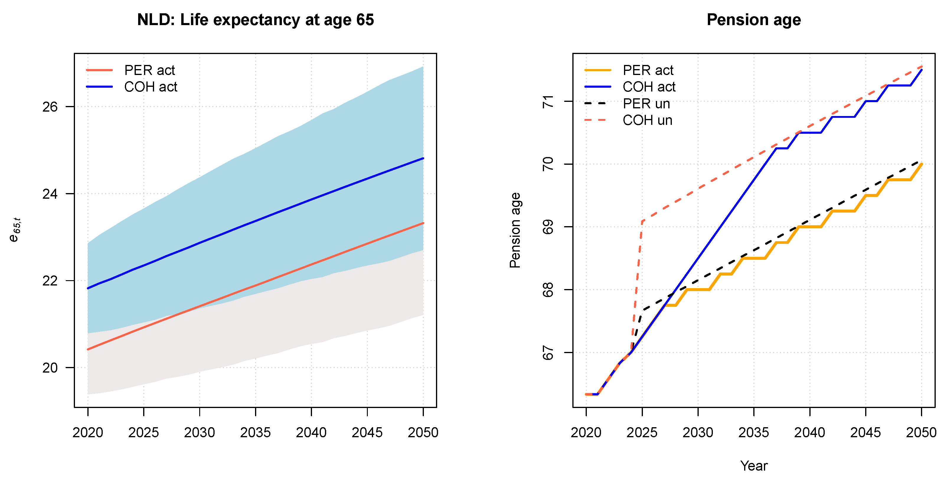
Figure 2 plots, for The Netherlands, the BME forecast of the period and cohort unisex life expectancy measures at the reference indexation age (age 65) from year 2020 to year 2100 (year 2050 for cohort longevity measures) along with 95% MATA prediction intervals (left panel). In addition, the point forecast of the standard pension age is computed using two estimates: the period (PER act) pension age, i.e., formula (5), which is the formula used in practice in The Netherlands, and a counterfactual scenario based on cohort (COH act) unisex life expectancy at age 65 is used in applying the same indexation rule (right panel, solid lines). The dashed lines refer to the point forecast of the standard pension age computed using Equation (5) and the period and cohort life expectancy estimates in a counterfactual scenario where the provisions currently in force in The Netherlands limiting the maximum increase per period and/or increasing with an indexation lag did not apply. This serves the purpose of highlighting the importance of additional design features in the overall policy outcome, which are particularly relevant in the case of The Netherlands and Denmark. Numerical values for selected years are provided in Table 2. The Dutch period (cohort) life expectancy at age 65 is forecasted to increase from 20.42 (21.82) years in 2020 to 23.32 (24.81) years in 2050. The conclusion is that the life expectancy gap between the choice of period and cohort life expectancy will grow from 1.40 years in 2020 to 1.49 years in 2050, a result that translates into an approximate implicit tax in the coming 30 years of 7%.15
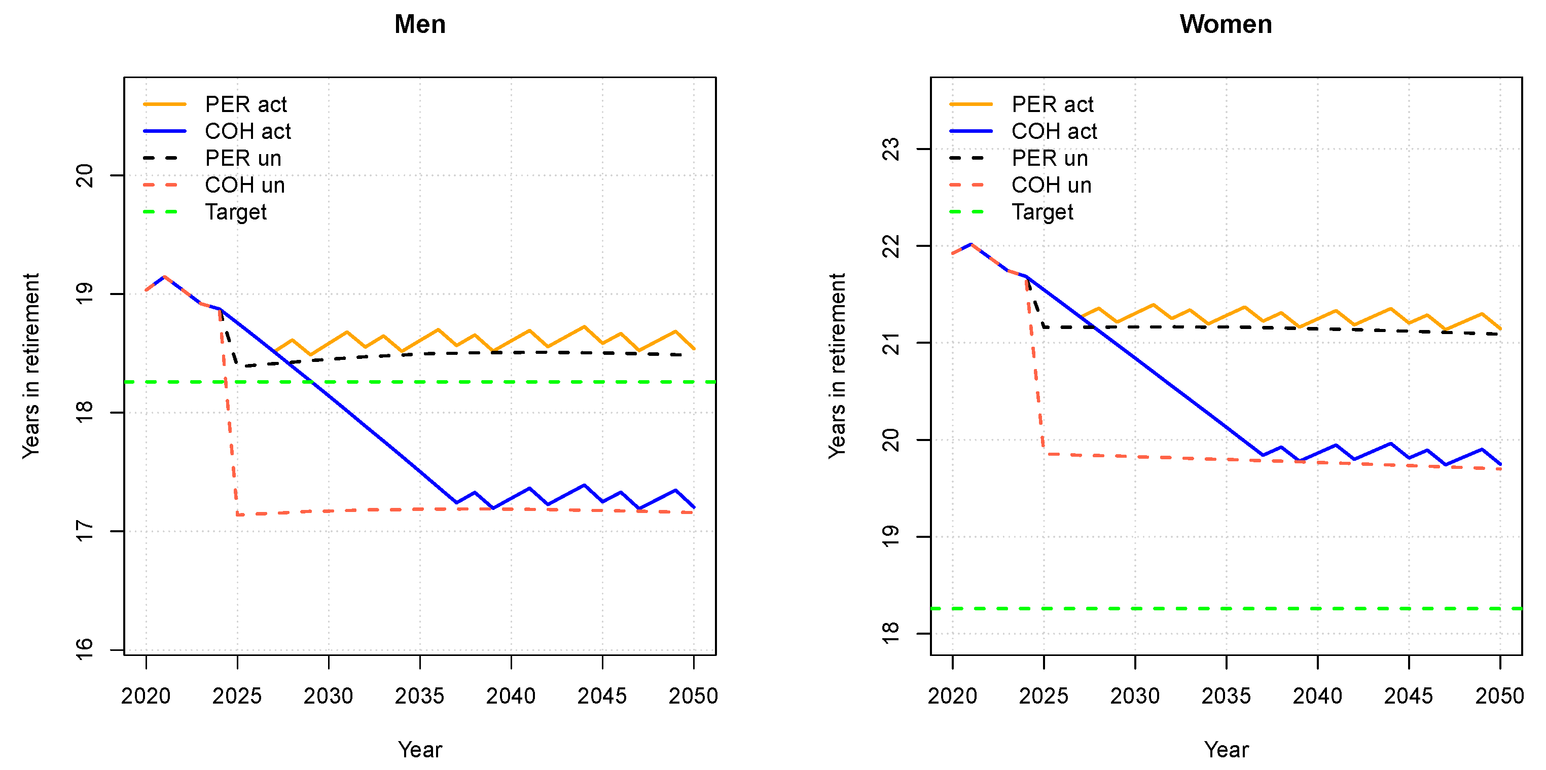
Summing up, the standard Dutch pension age is forecasted to increase from the current 66.33 years in 2020 to 68 years in 2030, 69 years in 2040, 70 years in 2050 and to 74 years by 2100, using the indexation formula which is based on period life expectancy. In the counterfactual scenario in which cohort life expectancy at age 65 is used in (5), we forecast that the pension age would increase to 68.5 years in 2030, 70.5 years in 2040 and 71.5 years in 2050, i.e., an extra increment of 1.5 years when compared to that obtained using period life expectancy. In the counterfactual scenario in which both the present «cap» provision and the indexation lag are ignored, our cohort-based projections (in parentheses) predict that the standard pension age should increase faster than the actual period-based formula predicts. Already in the first decade to the year 2030, the differences are 68.15 (69.60) years in 2030. The differences continue to increase to 69.11 (70.60) years in 2040 and 70.06 (71.55) years in 2050 if the period instead of cohort life expectancy is used. Figure 3 plots the expected years in retirement by gender computed using the cohort life expectancy estimated at that age, under the above policy design scenarios, together with the 18.26 years target. As of 2020, Dutch men (women) are expected to live 19.03 (21.92) years in retirement considering the legislated indexation rule, a result well above the 18.26 years embedded in current policy.
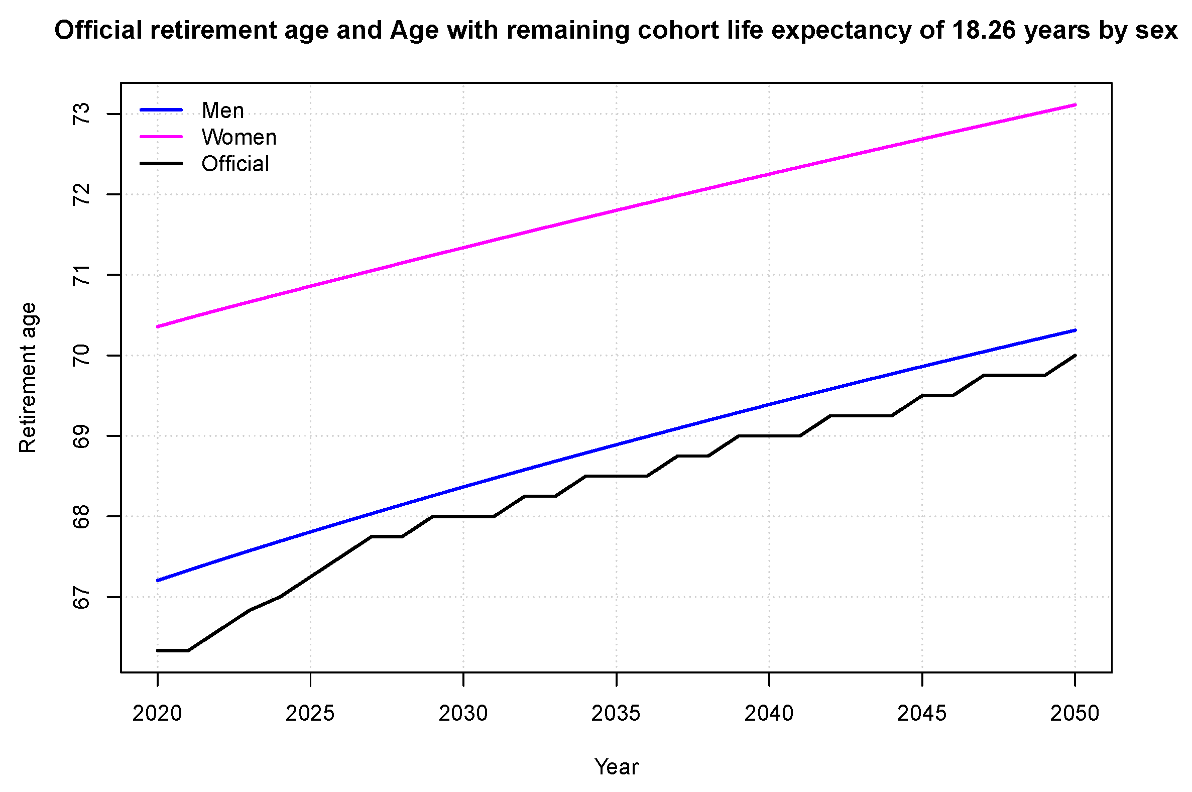
The expected benefit duration is forecasted to drop to 18.76 (21.54) years for men (women) in 2025, when the indexation rule comes into force, and will remain stable around 18.60 (21.30) years for men (women) until 2050—nevertheless always above the target benefit duration. The key conclusion is that the use of cohort instead of period life expectancy in the indexation formula and the elimination of The Netherlands’ «extra provisions» would significantly reduce the expected years in retirement to 17.15 (19.70) years for men (women) in 2050, well aligned with the 18.26 years (total population) target. Finally, Figure 4 plots the forecast of the official (legislated) desired standard retirement age and age with remaining cohort life expectancy equal to the 18.26 years target, plotted by sex.
Assuming that individuals retire at the normal retirement age, our results show that, as of 2020, the retirement age would need to increase to 67.20 years for men and 70.36 years for women to be consistent with the target expected benefit duration as expressed in policy (5). We forecast that the retirement age would need to increase to 70.31 years for men and 73.11 years for women in 2050 to match pension policy objectives. As Figure Figure 4 shows, the projections needed to fulfill an intergenerational neutral policy are consistently above the legislated age.

3.2. Denmark

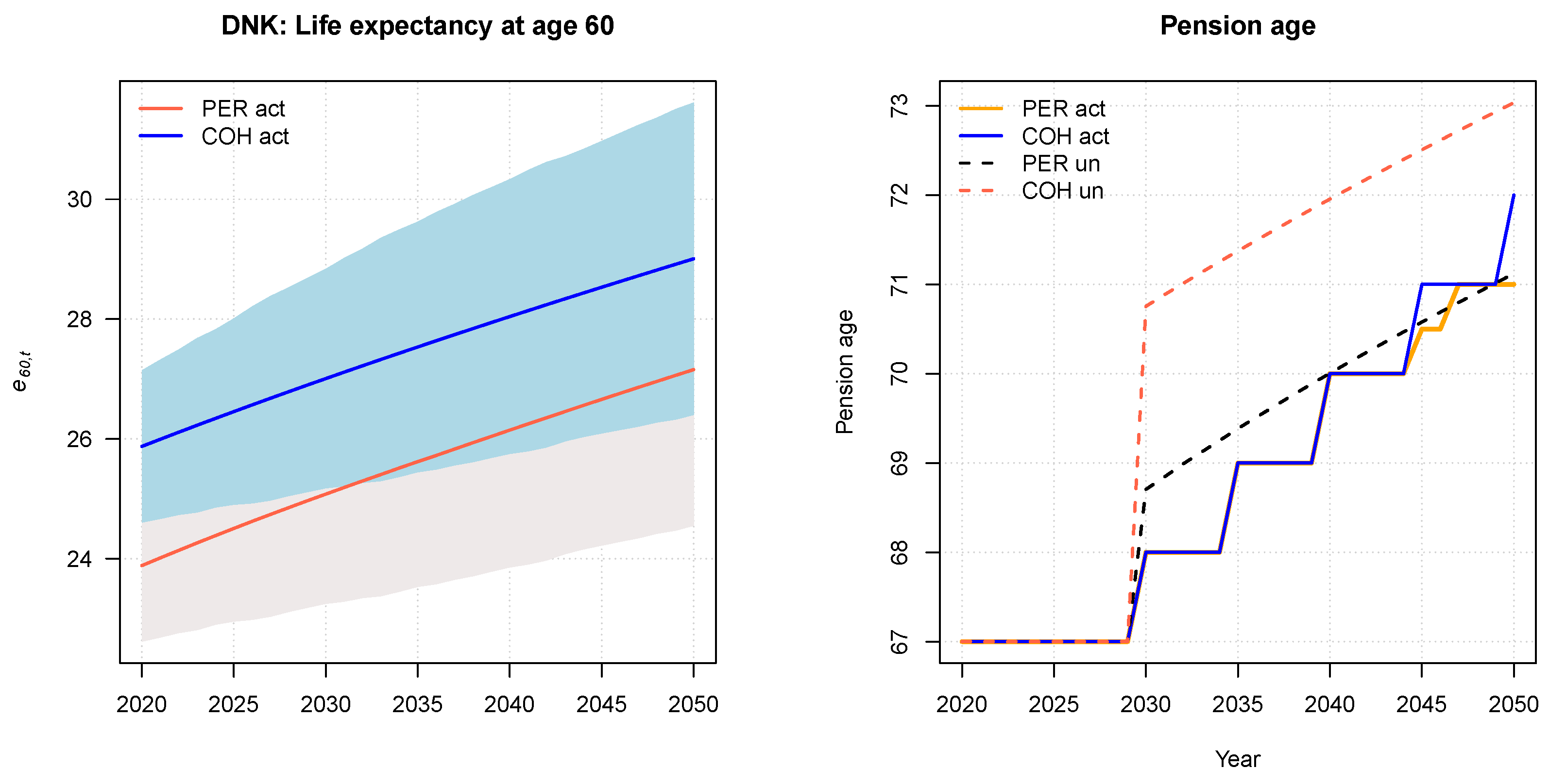
Figure 5 plots, for Denmark, the BME forecast of the unisex period and cohort life expectancy measures at age 60 along with 95% prediction intervals (left panel), together with the point forecast of the standard pension age computed using the actual Danish pension age formula (7) and a counterfactual scenario in which the cohort instead of period life expectancy is used in the indexation rule (right panel, solid lines). The dashed lines keep their previous meaning. Numerical values for selected years are provided in Table 3.
We forecast that the Danish period (cohort) life expectancy at age 60 will increase from 23.88 (25.87) years in 2020 to 27.15 (29.00) years in 2050, with a significant positive life expectancy gap of 1.85 years in 2050. The estimated life expectancy gap translates into a significant implicit tax from current to future generations ranging between 8.3% in 2020 and 6.8% in 2050. The Danish pension age (given the current indexation formula) is forecasted to increase from 67 years in 2020 to 71 years in 2050 and to 76 years by the end of the century. In the counterfactual scenario in which cohort life expectancy at age 60 is used in (7), we forecast that the pension age would increase to 72 years in 2050, i.e., one extra year when compared to that obtained using the legislated formula. Compared to the Dutch example, the pension age increases in Denmark are mitigated by the provision that limits retirement age increments to one extra year every 5 years and the longer indexation lag. In the counterfactual scenario in which both the cap and the 15-year indexation lag provisions are ignored, we forecast that the pension age would increase much faster than the legislated rule predicts to 68.70 (70.76) years in 2030, 70.00 (71.96) years in 2040 and 71.12 (73.03) years in 2050 if period (cohort) life expectancy is used.
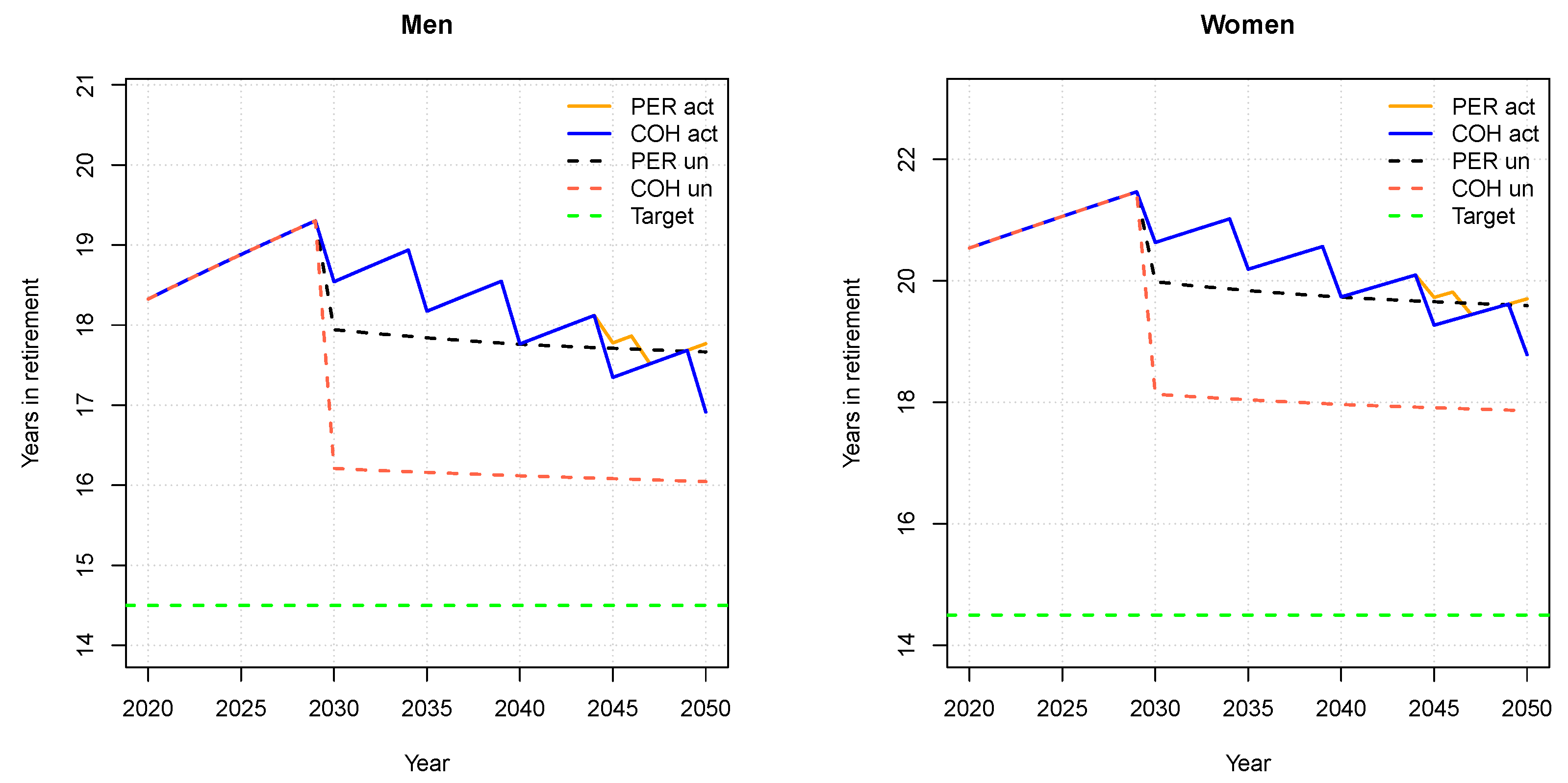
As of 2020, Danish men (women) are expected to live 18.33 (20.54) years in retirement considering the legislated indexation rule, a result well above the 14.5 years targeted by the policy (Figure 6). As a result of pension age increases, the expected benefit duration is forecasted to drop slightly to 17.77 years for men and 19.70 years for women in 2050, well beyond the policy target.
The use of cohort instead of period life expectancy in the indexation formula and the elimination of the extra provisions would significantly reduce the expected years in retirement to 16.05 (17.86) years for men (women) in 2050, a reduction which in any case would be insufficient to bring the expected benefit duration back to the 14.5 years target.
Indeed, our results show (Figure 7) that, as of 2020, the retirement age would need to increase to an astonishing 71.64 years for men and 73.95 years for women to be consistent with an expected benefit duration of 14.5 years. We forecast the retirement would need to increase to 74.92 years for men and 77 years for women in 2050 to match pension policy objectives, well above the predicted 71 years considering the legislated indexation rule.

3.3. Portugal

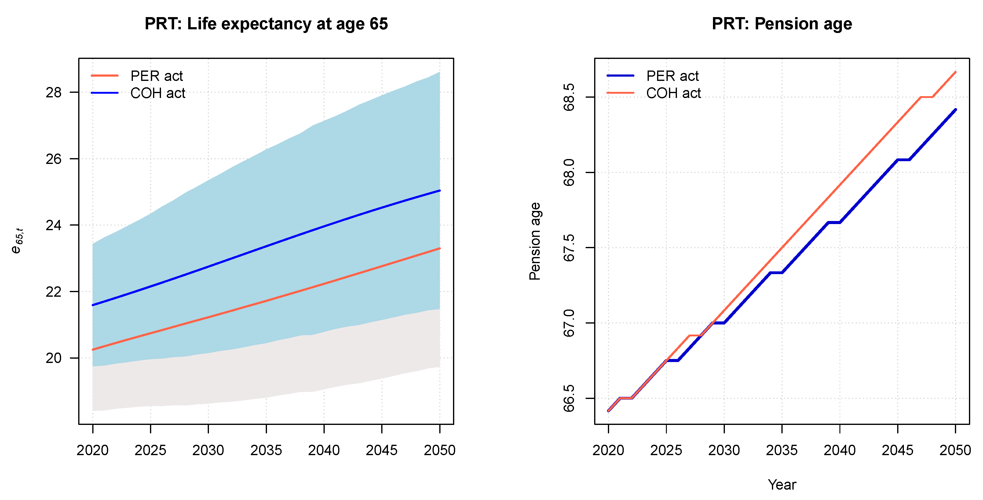
Figure 8 plots, for Portugal, the BME forecast of the unisex period and cohort life expectancy measures at age 65 along with 95% prediction intervals (left panel), together with the point forecast of the standard pension age computed using the actual pension age formula (8) and a counterfactual scenario in which the cohort instead of period life expectancy is used in the indexation rule (right panel). Numerical value for selected years are provided in Table 4. The unisex period (cohort) life expectancy at age 65 is forecasted to increase from 20.25 (21.59) years in 2020 to 23.30 (25.04) years in 2050 and to 27.54 years (period) in 2100. As a result, the Portuguese standard retirement pension age (considering the current indexation formula) is forecasted to increase from the current 66.41(6) years for both men and women in 2020 to 68.41(6) years in 2050 and to 71.3 years by the end of the century.
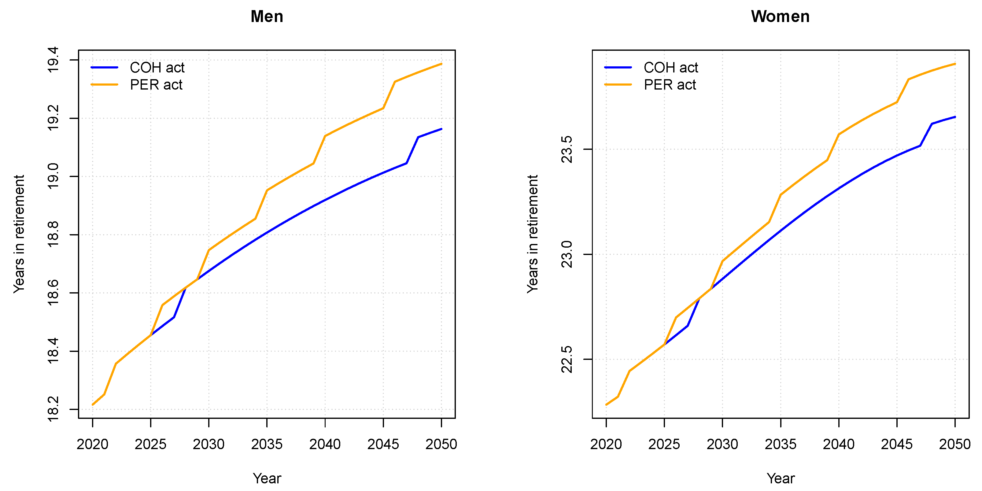
In the counterfactual scenario in which cohort life expectancy at age 65 is used in (8), we forecast the pension age would increase to 68.66 years in 2050, only three months higher than that obtained using the legislated formula. This means the indexation mechanism adopted in Portugal to update retirement age along with longevity developments is less sensitive to the choice of a particular life expectancy measure and will generate different pension ages only when trends in period and cohort life expectancy significantly deviate. In addition, the retirement age policy adopted, splitting the burden of longevity increments between active life and retirement, results in smaller pension age increases when compared to the Dutch and Danish cases which target a constant period in retirement. As of 2020, Portuguese men (women) are expected to live 18.22 (22.28) years in retirement considering the legislated indexation rule (Figure 9).
Our results show that, despite the expected retirement age increases, the duration of pension benefits is forecasted to substantially increase to 19.39 years for men and 23.91 years for women in 2050. This is a consequence of the retirement age policy pursued that extends working life only by two thirds of life expectancy developments observed at age 65.

3.4. Slovakia

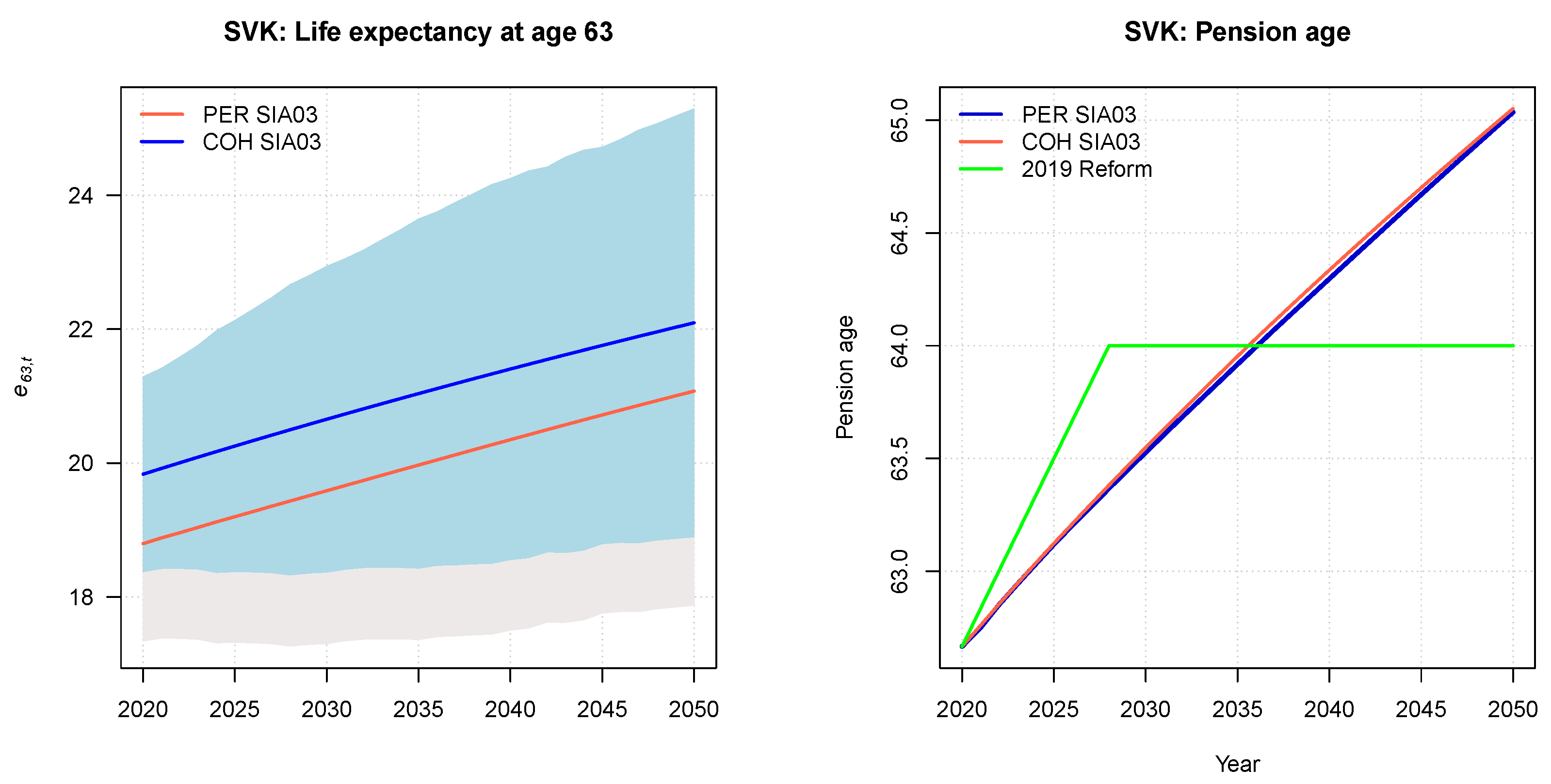
Figure 10 plots, for the Slovak Republic: (i) the BME forecast of the unisex period and cohort life expectancy measures at age 63 along with 95% prediction intervals (left panel); (ii) the point forecast of the standard pension age computed using the pension age formula (11) introduced by the Social Insurance Act of 2003 (SIA03), abandoned in 2019; (iii) a counterfactual scenario in which the cohort instead of period life expectancy is used in the indexation rule; and (iv) the new 2019 legislated retirement age (right panel). Numerical value for selected years are provided in Table 5.
The unisex period (cohort) life expectancy at age 63 is forecasted to increase from 18.80 (19.83) years in 2020 to 21.07 (22.09) years in 2050 and to 24.04 in 2100 (using the period approach). As a result, the standard pension age resulting from the SIA03 Act was forecasted to increase from the current 62.6(6) years for both men and women in 2020 to 65.04 years in 2050 and to 67.97 years by the end of the century. The 2019 reform caps the retirement age at 64 years, well below the previous path. Our results show that, if cohort life expectancy had been used in (11), the retirement age path would be very similar to that obtained using the period approach. This may suggest that Slovakia has yet to experience any considerable acceleration in the rate of decline in mortality at older ages, which is a driver of the scale of the gap between cohort and period projections.
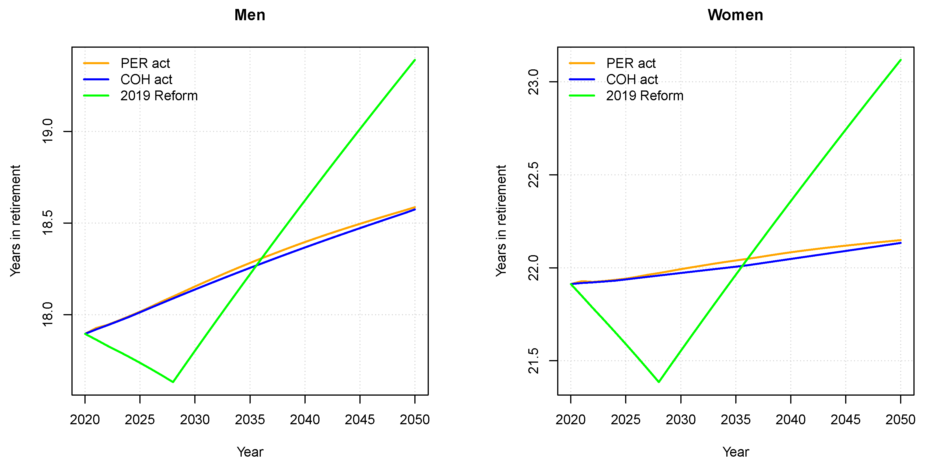
As of 2020, men (women) retiring in Slovakia are expected to live 17.90 (21.91) years in retirement considering the legislated pension age (Figure 11).
We forecast the expected benefit duration would have increased to 18.59 years for men and 22.15 years for women in 2050 if the Social Insurance Act of 2003 had remained in force, but the 2019 reform reversal capping the retirement age at 64 years will augment the years in retirement to 19.39 for men and to 23.12 years for women on the same date, challenging the long-term sustainability of the pension scheme.

4. Discussion and Conclusions

The purpose of linking retirement ages to life expectancy developments is chiefly to minimize the impact of demographic and economic shocks on the financing of pension schemes. In addition, there is also an implicit objective which is to introduce economic/actuarial rationality for justifying changes, avoiding the thorns of regular political negotiations to adopt the required adjustments. This replaces necessary ad hoc measures and, by doing so, enhances the credibility of the system by preventing otherwise unexpected public finance crises in the future. However, the way that the biometric indicators have been introduced in national pension schemes suggests that there are several possible flaws, sometimes including the use of inappropriate longevity measures. In this paper, we pay special attention to four countries—The Netherlands, Denmark, Portugal, and Slovakia)–that have recently introduced an automatic link between the statutory (standard) retirement age and life expectancy. In three of the four countries–where Slovakia most likely because of the absence of acceleration in the rate of improvement in life expectancy is the exception—our results demonstrate that legislated pension ages deviate from target policy outcomes due to the way policy has been designed and implemented.
We forecast statutory retirement ages for selected countries using a novel adaptative BME approach (Bravo et al. 2021a). Based on results for The Netherlands, Denmark and Portugal, two factors appear to be at work. First, the use of period life instead of cohort life tables inevitably leads to an underestimate of remaining life at retirement; and, second, provisions limiting the maximum increase per period and/or indexation with lags. These smooth pension age increases but postpone the adjustments required to achieve the policy outcome.
The four countries analyzed in this study have automatically indexed the standard retirement age to unisex period life expectancy but pursued alternative retirement age policies. In Denmark and in The Netherlands, the choice was to set the retirement age such that individuals in successive birth cohorts of retirees are expected to enjoy on average a constant number of years in retirement, i.e., all expected additional years of life (computed from a given constant age) will be spent in work rather than in retirement. However, in both countries, the policy option of using period instead of cohort life expectancy measures to estimate the remaining lifetime at retirement nevertheless results in systemic differences between the official standard pension age and the target pension age, thereby undermining policy ambitions.
In addition, in both countries, the legislated retirement age indexation formula includes provisions limiting the maximum increase per period, and with significant indexation lags. For example, in Denmark, every five years, regulations for the cap need to be approved by a majority in the Danish parliament with 15 years notice and adjustments are smoothed over time. This generates an additional deviation between the actual and the target number of years in retirement.
In Portugal, the adopted retirement age policy splits the burden of longevity improvements observed at age 65 between years of work and retirement with a time lag of two years. This means that in the aggregate this costs the country two years of income per retiree if all take advantage of the extra two years to increase their “leisure” use of time.
We also note here that, in Slovakia, the 2012 pension reform, effective from 2017 and abandoned in 2019, adopted a retirement age policy by which the retirement age updates on a one-to-one basis according to the year-on-year difference (in days) of the 5-year moving average of the unisex period life expectancy computed at current standard retirement age.
The main conclusions from our results are different for each analyzed country depending on the specific policy design adopted against the desired policy outcomes. In countries that, like The Netherlands and Denmark, have opted to target a constant period in retirement, our results confirm a significant deviation between the forecasted benefit duration and the target period in retirement defined when linking the retirement age to life expectancy. In both countries, deviations are observed in two main contexts. First, life expectancy at the reference indexation age is actually higher than that estimated when the mechanism was first implemented—which occurs regardless of whether the period or cohort approach to projecting life expectancy has been taken, but the gap between the estimate and the outcome is likely to become considerably larger if the country employs the period approach. Second, if—or more likely when—improvements in mortality begin to accelerate for persons in their 80s and 90s, the expected number of years in retirement can substantially increase in the coming decades, and the current adjustment mechanisms are unable to offset these expected increases.
In both countries, replacing period with cohort projection techniques for estimating life expectancy would help to bring results closer to those targeted by current retirement age policies, while cohort projections (and consequently a higher reduction in expected years in retirement) would bring results closer to the desired outcome of reconciling pension system sustainability and adequacy in the context of ageing populations. Notably, the retirement ages with remaining cohort life expectancy of 18.26 years in The Netherlands and 14.5 in Denmark are higher than the official retirement age actually established.
The automatic indexation rule for the pension age works differently in Portugal and the Slovak Republic. In both countries, the pension age path is less sensitive to the use of a period instead of a cohort approach when computing life expectancy estimates. The adopted policy design will only generate significant bias if trends in period and cohort life expectancy substantially deviate over time. However, contrary to The Netherlands and Denmark, whose policy strives to stabilize expected years in retirement of successive birth cohorts, the retirement age policies adopted in Portugal and Slovakia will not freeze increases in the expected number of years of benefit duration–even with a cohort approach to projecting the value of life expectancy to be used in indexing the pension age, challenging the long-term financial sustainability of the pension scheme. As has already been noted, there is nevertheless a trade-off between longer periods of retirement going forward with a constant number of years of work and, by definition, in the context of a defined benefit scheme, where, in the aggregate, it is the younger generation that pays for the premium, which comes at the expense of lower GDP for all.
In the case of the Slovak Republic, the 2019 reform reversal capping the retirement age at 64 years will by definition lead to an increase in the number of years in retirement compared with the expected outcome of the previous regulation. According to our calculations, the model replaced was able to correct for the LE gap between period and cohort projections for the life expectancy, with similar results for the pension age path according the two methodologies and, thus, a similar number of projected for years in retirement. As we have already commented, this can be attributed to the absence of acceleration in the rate of decline in mortality in older ages—which if and when it occurs would speak in favor of the cohort estimation model. This emphasizes the superiority of nevertheless employing the cohort projection because it is at least as good as the period model and becomes increasingly superior in the face of the extended periods of accelerating mortality improvement in higher ages, which is likely to characterize Slovakia in the not-so-distant future.
It is important for all actors in the economy to be able to foresee the future evolution of a country’s standard pension age(s) for national public pension commitments. First, and foremost, this is important for maintaining the affordable, financially sustainable and intergenerationally fair pensions. Second, rules that determine the standard retirement age interact with other social benefit schemes, and private pension schemes that for some (most frequently persons with higher income/savings) yield a substantial supplement to the national scheme—depending on the ceiling for contributions/benefits from the national scheme. In this context, it makes a difference whether the scheme is a DB or a DC scheme—and the values of the design parameters—not the least ceilings affecting contributions (per definition in DC schemes) or benefits (per definition in DB schemes).
Third, stability and transparency in public schemes are important for the retirement plans of individuals. «The pension age» and the accompanying information on the consequences of the decisions of individuals to exit the labor market constitute an important input into individual decisions weighing the merits of longer working lives weighed against a desire for leisure. In turn, these decisions are reflected in the scale of the labor force and thus society’s GDP. In this context, DC schemes transmit a clear signal, whereas DB schemes only do this reliably (as the terms of the contract may be subject to change) unless they de facto mimic DC schemes. Fourth, longer working lives for healthy individuals approaching the retirement age affect labor supply and economic growth—this is a reality that must be covered by supporting social insurance (disability) policy. The last point here is crucial because increases in life expectancy are not necessarily accompanied by equivalent increases in healthy life expectancy for all. Work at increasingly higher ages will be problematic for many.
Finally, the research of Chetty et al. (2016) and a cross-discipline undertaking of the US National Academies of Sciences, Engineering, and Medicine (2015) suggest that the underlying causes—in the US—are systemic socio-economic disparities grounded in health impeding lifestyles and the absence of community social service support. Although not as dramatic, studies performed in Europe reveal a pattern that is similar to that in the US. In the long term, this sort of national profile calls for considerable social investments in public health reaching people in the early stages of life when long-term health and economic prospects of individuals throughout their working lives are all too often determined. In the short-term, this may justify designing benefits so as to accommodate socio-economic differentials. Work in this direction has already started (see, e.g., Holzmann et al. 2020), but this is definitely a topic for future work.

Author Contributions

Conceptualization, M.A., J.M.B., R.H., and E.P.; methodology, M.A., J.M.B., R.H., and E.P.; software, M.A., J.M.B., R.H., and E.P.; validation, M.A., J.M.B., R.H., and E.P.; formal analysis, M.A., J.M.B., R.H., and E.P.; investigation, M.A., J.M.B., R.H., and E.P.; writing—original draft preparation, M.A., J.M.B., R.H., and E.P.; writing—review and editing, M.A., J.M.B., R.H., and E.P.; All authors have read and agreed to the published version of the manuscript.

Funding

This research was funded by the Spanish Ministry of Science and Innovation for funding received under grant PID2019-105986GB-C21 (Mercedes Ayuso) and by Portuguese national science funds through FCT under the grant UIDB/04152/2020—Centro de Investigação em Gestão de Informação (MagIC) (J.M. Bravo).

Institutional Review Board Statement

Not applicable.

Informed Consent Statement

Not applicable.

Data Availability Statement

Not applicable.

Acknowledgments

The authors would like to express their gratitude to the anonymous referees for his or her careful review and insightful comments that helped strengthen the quality of the paper. We are also thankful for the suggestions and remarks from participants at the WorldCIST’21 Conference, Azores, Portugal.

Conflicts of Interest

The authors declare no conflict of interest.

Appendix A. Stochastic Mortality Models: Technical Description

This section draws heavily on Bravo et al. (2021a) and provides a brief technical description of the individual stochastic mortality models considered in the Bayesian Model Ensemble approach. It is included in the paper for completeness.

Appendix A.1. GAPC Stochastic Mortality Models

Generalised Age-Period-Cohort (GAPC) mortality models are a class of parametric models that link a response variable with a linear or bilinear predictor structure consisting of a series of factors dependent on age of the individual, x; period effects, t; and year of birth (or cohort) effects, c = t x . GAPC models fit into the general class of generalized nonlinear models (GNM), with a structure that includes a random component, a systematic component, a link function, a set of parameter constraints to ensure identifiability, and time series methods for forecasting and simulating the period and cohort indexes (see, e.g., Hunt and Blake (2021) for a review). The random component specifies whether the number of deaths recorded at age x during calendar year t , D x , t , follows a Poisson distribution D x , t P μ x , t E x , t c , with E D x , t / E x , t c = μ x , t , or a Binomial distribution D x , t B q x , t E x , t 0 , with E D x , t / E x , t 0 = q x , t , where E x , t 0 and E x , t c denote, respectively, the population initially or centrally exposed-to-risk, and q x , t is the one-year death probability for an individual aged x last birthday in year t . The systematic component links a response variable to an appropriate linear predictor η x , t
η x , t = α x + i = 1 N β x ( i ) κ t ( i ) + β x ( 0 ) γ t x ,
where exp α x denotes the general shape of the mortality schedule across age, β x ( i ) κ t ( i ) is a set of N age-period terms describing the mortality trends, with each time index κ t ( i ) contributing to specifying the general mortality trend and β x ( i ) modulating its effect across ages, and the term γ t x γ c accounts for the cohort effect c with β x ( 0 ) modulating its effect across ages. The age modulating coefficients β x ( i ) can be preset or non-parametric terms to be estimated, e.g., as in the Lee–Carter model. The period indexes κ t ( i ) and the cohort index γ t x are stochastic processes. The link function g connects the random component and the systematic component, i.e., g E D x , t / E x , t = η x , t , typically following the canonical link. The specification is complemented with a set of parameter constraints to ensure unique parameter estimates. Parameter estimates are obtained using maximum-likelihood (ML) methods. To forecast and simulate mortality rates, we assume that the age vectors α x and β x ( i ) remain constant over time and model period indices κ t ( i ) using a multivariate random walk with a drift. Cohort indices γ t x were modelled with general univariate ARIMA ( p , d , q ) models with drift. Box–Jenkins methodology (identification-estimation-diagnosis) is used to estimate the appropriate ARIMA model.

Appendix A.2. Weighted Hyndman–Ullah Method

The Hyndman and Ullah (2007) method combines nonparametric penalized regression spline with functional principal component analysis for modelling and forecasting log mortality rates. The authors assume that the logarithm of the observed mortality rate at age x x 1 , x p in year t t 1 , t n , log m x i , t y t x i , is a realization of an underlying continuous and smooth function f t x i that is observed with error at discrete ages, i.e.,
y t x i = f t x i + σ t x i ε t , i , i = 1 , , p t = 1 , , n ,
where σ t x i allows the amount of noise to vary with x i in year t, thus rectifying the assumption of homoscedastic error in the LC model, and ε t , i is an independent and identically distributed standard normal random variable. The log mortality rates are smoothed prior to modelling using penalized regression splines with a partial monotonic constraint. Using functional PCA, the smoothed mortality curves I = y 1 x , , y n x are then decomposed into orthogonal functional principal components and their uncorrelated principal component scores. In this paper, we use the weighted Hyndman–Ullah (HUw) extension proposed in Shang et al. (2011) which differs from the original HU method in that it uses geometrically decaying weights in the estimation of the model parameters. Formally,
f t x = a ^ * x + j = 1 J b j * x k t , j + e t x ,
where a ^ * x is the weighted functional mean age function estimated by
a ^ * x = 1 n j = 1 J w t f t x , j = 1 J w t = 1 ,
where w t = π 1 π n t , t = 1 , , n denotes a set of weights, and π 0 , 1 refers to the geometrically decaying weight parameter, with an optimal value chosen so as to minimize an overall forecast error measure within the validation data; B * = b j * x j = 1 , , J is a set of weighted first J functional principal components with uncorrelated principal component scores k t , j derived by functional principal component analysis from the set of weighted curves w t f t x a ^ * x ; t = 1 , , n ; e t x is the residual function with mean zero and variance υ x estimated by averaging e 1 2 x , , e n 2 x , e t x N 0 , υ x ; and J < n is the number of principal components used. Following Shang et al. (2011), we chose J = 6 .

Appendix A.3. CP-Splines Model

The CP-spline model is an extension of the two-dimensional P-splines model proposed by Currie (2006) through incorporating demographic constraints to ensure that future mortality over the whole age range follows a plausible and well-behaved demographic profile when estimated from past data (Camarda 2019). Consider a mortality dataset comprising deaths and exposure-to-risk arranged in two m × n matrices, Y = d i j and E = E i j , respectively, with rows and columns classified by single age at death, x, m × 1 and single year of death, t, n × 1 , respectively. The approach assumes that the number of deaths d i j at age i in year j is Poisson-distributed with mean μ i j E i j , i.e., d i j P μ i j E i j . The goal is to model and forecast mortality over both age and time combining (fixed knot) B-splines with a roughness penalty to achieve a compromise between fitting accuracy and smoothness. Let B x , m × k x and B t , n × k t be the B-splines over ages and years, respectively. The log mortality is described as a linear combination of B-splines and associated coefficients ( α ):
ln [ E ( Y ) ] = ln ( E ) + B α
where ln ( E ) is the offset and η = B α is the linear predictor. The regression matrix for the two-dimensional model is given by the Kronecker product of the k equally spaced B-splines bases for age x and year t , B = B t B x , where ⊗ denotes the Kronecker product of two matrices. The two-dimensional penalty is given by
P = λ x I k t D x D x + λ t D t D t I k x ,
where λ x and λ t are the smoothing parameters used for age and year, respectively; I k x and I k t are identity matrices of dimension k x and k t , respectively; and D x and D t are difference matrices over the rows (ages) and columns (years) of the coefficient matrix. The author adds shape constraints and asymmetric penalties on the rate of aging (relative derivatives of the age mortality profile), D x t , and on the rate of change of mortality rates over time, D t t , to enforce mortality patterns over age and time. We derive confidence intervals for forecasted mortality rates by carrying out a residual bootstrap of the fitted model.

Appendix A.4. Regularized SVD Model

The Regularized SVD (RSVD) approach extends one-way functional principal component analysis (PCA) to two-way functional data by introducing regularization of both left and right singular vectors in the singular value decomposition (SVD) of the data matrix (Huang et al. 2009; Zhang et al. 2013). Formally, the mortality rate at age x in year t is given by
m x , t = j = 1 q d j U j t V j x + ε x , t ,
where d q is the singular value, U i · and V j · are smooth functions of period and age, respectively, and ε x , t is a mean zero random noise. The model is fitted iteratively. The first pair of singular vectors of a data matrix X = m x , t n × p , U 1 t and V 1 x , whose discretized realizations are, respectively, denoted as u 1 U 1 t 1 , , U 1 t n T and v 1 V 1 x 1 , , V 1 x p T , is obtained by solving a least squares problem as
u ^ , v ^ = arg min u , v X uv T F 2 ,
where · F is the Frobenius norm of a matrix. Subsequent pairs are extracted sequentially by removing the effect of preceding pairs. For two-way functional data, the RSVD of Huang et al. (2009) defines the regularized singular vectors as
u ^ , v ^ = arg min u , v X uv T F 2 + P λ u , v ,
where P λ u , v is a regularization penalty
P λ u , v = λ u u T Ω u u · v 2 + λ v v T Ω v v · u 2 + λ u u T Ω u u · λ v v T Ω v v ,
where Ω u n × n and Ω v p × p are symmetric and nonnegative definite domain-specific penalty matrices, whose purpose is to balance goodness-of-fit against smoothness, and λ is a vector of regularization parameters optimally estimated based on generalized cross-validation (GCV) criterion. To forecast mortality rates and derive confidence intervals, we treat the time functions U i t as time series and model them using general univariate ARIMA processes, rescaling the pairs in (A7) by the ratio d i / d 1 , i = 2 , , q . We account for parameter uncertainty in the construction of prediction intervals adopting a semiparametric bootstrap approach.

Appendix B. Life Expectancy Gap and Implied Tax/Subsidies

The estimated magnitude of the life expectancy gap at the retirement age and its ratio against period life expectancy can be given a welfare economic interpretation through the concept of pension wealth in an intergenerational actuarial fairness setting (Ayuso et al. 2021; Bravo et al. 2021a). Assuming that the benefit indexation equals the discount rate, i.e., π t = y t t , the life expectancy gap amounts to a ex-ante tax/subsidy, S x r , g t , i.e.,
S x r , g t : = e ˙ x r , g G a p t e ˙ x r , g P ( t ) × 100 = e ˙ x , g C t e ˙ x r , g P ( t ) 1 × 100 ,
that a given generation would pay/receive unless (initial or subsequent) benefit adjustments are undertaken to make the system actuarially fairer. In Equation (A11), negative values represent a tax rate and positive values a subsidy rate to current generations. Stated differently, the larger the life expectancy gap, the more pension benefits depart from an intergenerationally fair and neutral pension scheme.

Notes

1
For a detailed discussion of pensions taxation, see, e.g., Holzmann and Piggott (2018) and Bravo (2016).
2
In private individual or employer-sponsored pension plans, diverse insurance and non-insurance longevity risk-sharing mechanisms (e.g., Group-Self Annuitization schemes, longevity-linked life annuities, tontine annuities) have also been proposed and some successfully implemented (Piggott et al. 2005; Valdez et al. 2006; Stamos 2008; Milevsky and Salisbury 2015; Bravo and El Mekkaoui de Freitas 2018; Bravo 2019, 2020, 2021).
3
Spain suspended the adjustment of pension benefits with the life expectancy sustainability factor in 2019 at least until 2023.
4
The standard, normal or also full retirement age is defined here as the age at which individuals can first withdraw their full pension benefits, i.e., without actuarial decrements (reductions) or increments (bonus) for early (late) retirement. In most countries, standard pension ages are clearly defined in legislation. In many countries, different standards apply to different components of the overall retirement-income package. In addition, many countries have specific provisions allowing individuals to retire earlier than the standard age with full benefits given that certain contribution requirements are met. We note that some countries have opted not to have a “standard” retirement age, defining instead an age window at which pension benefits may first be drawn.
5
In the last two decades, nearly all European countries have augmented the standard and early retirement ages (the only exception being Luxembourg), with particularly large increases legislated in some cases (e.g., Greece, Sweden, France and Finland). Some countries have limited or slowed down the increase in the retirement age following reforms adopted in the past (Italy, The Netherlands, and the Slovak Republic).
6
For instance, in the United States, only those reaching age 65 are entitled to Medicare. Those who retire earlier receive less than full social security pension benefits and will have no employer and no Medicare health coverage during the years from retirement prior to age 65. This discourages workers from retiring at a younger age to avoid an extra pension decrement.
7
Turkey has already announced it will phase out the sex difference for those entering the labour market in 2028.
8
There are some notable exceptions to this pattern, namely, South Korea and Turkey, where the effective labour market exit age is considerably higher than the standard retirement age for both men and women. In recent years, we have seen some reform reversals in this area, with some countries (e.g., Italy and Portugal) easing early-retirement conditions. For instance, in 2019, Italy suspended until 2026 the automatic indexation of both the statutory retirement age and the career-length eligibility conditions for early retirement to life expectancy and expanded early retirement options by introducing the so-called “Quota 100” (which enables retirement at age 62 with 38 years of contributions until 2021 and allows combining work and pensions before the statutory retirement age, but subject to a labour-income ceiling) and the ”women’s option” which allows women to retire at age 58 with 35 years of contributions if they fully switch to the NDC benefit calculation.
9
10
The plan was to raise the eligibility age by one month per year between 2013–2015, three months per year between 2016–2018, and four months per year in 2019–2021, reaching the age of 67.2 by 2021 (European Commission 2019).
11
Decree-law 167-D/2013 from December 31.
12
The retirement age is kept at 65 years for beneficiaries legally prevented from working beyond that age (e.g., pilots, drivers of heavy vehicles). In addition, when the scheme participants reach the age of 65, the standard pensionable age is reduced by four months for each calendar year (with registered earnings) worked in excess of the contributions ceiling of 40 years, with a 60-year threshold. There are specific early retirement provisions for those with very long contribution careers, in long-term involuntary unemployment or working in certain arduous jobs (e.g., miners).
13
The SMAPE for model k and population g is defined by
S M A P E k , g : = 1 n x , t x = x min x max t = t min t max μ ˙ x , t , g μ x , t , g 0.5 × μ ˙ x , t , g + μ x , t , g ,
where μ ˙ x , t , g and μ x , t , g denote the point forecast and observed mortality rates, respectively, and n x , t = x max x min + 1 t max t min + 1 .
14
For instance, model LC is nested within model RH, with β x ( 0 ) = 0 for all x, and γ t x = 0 for all c , being a special case of APC with β x ( 1 ) = 1 for all x and no cohort effects. Model APC is a special case of RH with β x ( 1 ) = β x ( 0 ) = 1 for all x. The CBD model is a restricted version of M7 with κ t ( 3 ) = 0 for all t and γ t x = 0 for all c.
15
For computational details, we refer to Appendix B and to Ayuso et al. (2021).

References

  1. Alho, Juha, Jorge M. Bravo, and Edward Palmer. 2013. Annuities and life expectancy in NDC. In Nonfinancial Defined Contribution Pension Schemes in a Changing Pension World, Volume 2, Gender, Politics, and Financial Stability. Edited by Robert Holzmann, Edward Palmer and David Robalino. Washington, DC: World Bank, pp. 395–436. [Google Scholar]
  2. Arnold, Séverine, and Anca Jijiie. 2020. Retirement Ages by Socio-Economic Class. Risks 10: 102. [Google Scholar] [CrossRef]
  3. Auerbach, Alan J., Kerwin K. Charles, Courtney C. Coile, William Gale, Dana Goldman, Ronald Lee, and Charles M. Lucas. 2017. How the Growing Gap in Life Expectancy May Affect Retirement Benefits and Reforms. NBER Working Papers 23329. Cambridge: National Bureau of Economic Research, Inc. [Google Scholar]
  4. Ayuso, Mercedes, Jorge M. Bravo, and Robert Holzmann. 2017a. On the heterogeneity in longevity among socioeconomic groups: Scope, trends, and implications for Earnings-Related Pension Schemes. Global Journal of Human Social Sciences-Economics 17: 31–57. [Google Scholar]
  5. Ayuso, Mercedes, Jorge M. Bravo, and Robert Holzmann. 2017b. Addressing longevity heterogeneity in pension scheme design. Journal of Finance and Economics 6: 1–21. [Google Scholar] [CrossRef] [Green Version]
  6. Ayuso, Mercedes, Jorge M. Bravo, and Robert Holzmann. 2021. Getting Life Expectancy Estimates Right for Pension Policy: Period versus Cohort Approach. Journal of Pension Economics and Finance 20: 212–31. [Google Scholar] [CrossRef]
  7. Blackburn, Craig, and Michael Sherris. 2013. Consistent dynamic affine mortality models for longevity risk applications. Insurance: Mathematics and Economics 53: 64–73. [Google Scholar] [CrossRef]
  8. Bravo, Jorge M. 2016. Taxation of Pensions in Portugal: A Semi-Dual Income Tax System. CESifo DICE Report 14: 14–23. [Google Scholar]
  9. Bravo, Jorge M. 2019. Funding for longer lives: Retirement wallet and risk-sharing annuities. Ekonomiaz 96: 268–91. [Google Scholar]
  10. Bravo, Jorge M. 2020. Longevity-Linked Life Annuities: A Bayesian Model Ensemble Pricing Approach. In Proceedings of the Atas da 20a Conferência da Associação Portuguesa de Sistemas de Informação 2020. CAPSI 2020 Proceedings. Available online: https://aisel.aisnet.org/capsi2020/29 (accessed on 30 January 2021).
  11. Bravo, Jorge M. 2021. Pricing participating longevity-linked life annuities: A Bayesian Model Ensemble approach. European Actuarial Journal. [Google Scholar] [CrossRef]
  12. Bravo, Jorge M., and Najat El Mekkaoui de Freitas. 2018. Valuation of longevity-linked life annuities. Insurance: Mathematics and Economics 78: 212–29. [Google Scholar] [CrossRef]
  13. Bravo, Jorge M., and Jose A. Herce. 2020. Career breaks, Broken pensions? Long-run effects of early and late-career unemployment spells on pension entitlements. Journal of Pension Economics and Finance, 1–27. [Google Scholar] [CrossRef]
  14. Bravo, Jorge M., and João Pedro Vidal Nunes. 2021. Pricing Longevity Derivatives via Fourier Transforms. Insurance: Mathematics and Economics 96: 81–97. [Google Scholar] [CrossRef]
  15. Bravo, Jorge M., and Mercedes Ayuso. 2020. Previsões de mortalidade e de esperança de vida mediante combinação Bayesiana de modelos: Uma aplicação à população portuguesa. RISTI-Revista Iberica de Sistemas e Tecnologias de Informacao E40: 128–44. [Google Scholar]
  16. Bravo, Jorge M., and Mercedes Ayuso. 2021. Forecasting the retirement age: A Bayesian Model Ensemble Approach. In Trends and Applications in Information Systems and Technologies, WorldCIST 2021. Advances in Intelligent Systems and Computing. Edited by Á. Rocha, H. Adeli, G. Dzemyda, F. Moreira and A.M. Ramalho Correia. Cham: Springer, vol. 1365, pp. 123–35. [Google Scholar] [CrossRef]
  17. Bravo, Jorge M., Mercedes Ayuso, Robert Holzmann, and Edward Palmer. 2021a. Addressing the life expectancy gap in pension policy. Insurance: Mathematics and Economics 99: 200–21. [Google Scholar] [CrossRef]
  18. Bravo, Jorge M., Mercedes Ayuso, Robert Holzmann, and Edward Palmer. 2021b. Intergenerational actuarial fairness when longevity increases: Amending the retirement age. Scandinavian Actuarial Journal. Preprint to submit. [Google Scholar]
  19. Brouhns, Natacha, Michel Denuit, and Ingrid Van Keilegom. 2005. Bootstrapping the Poisson Log-Bilinear Model for Mortality Forecasting. Scandinavian Actuarial Journal 3: 212–24. [Google Scholar] [CrossRef]
  20. Brouhns, Natacha, Michel Denuit, and Jeroen K. Vermunt. 2002. A Poisson Log-Bilinear Regression approach to the construction of projected life tables. Insurance: Mathematics and Economics 31: 373–93. [Google Scholar]
  21. Cairns, Andrew J. G., David Blake, and Kevin Dowd. 2006. A two-factor model for stochastic mortality with parameter uncertainty: Theory and calibration. Journal of Risk and Insurance 73: 687–718. [Google Scholar] [CrossRef]
  22. Cairns, Andrew J. G., David Blake, Kevin Dowd, Guy D. Coughlan, David Epstein, Alen Ong, and Igor Balevich. 2009. A quantitative comparison of stochastic mortality models using data from England and Wales and the United States. North American Actuarial Journal 13: 1–35. [Google Scholar] [CrossRef]
  23. Camarda, Carlo Giovanni. 2019. Smooth constrained mortality forecasting. Demographic Research 41: 1091–130. [Google Scholar] [CrossRef]
  24. Chetty, Raj, Michael Stepner, Sarah Abraham, Shelby Lin, Benjamin Scuderi, Nicholas Turner, Augustin Bergeron, and David Cutler. 2016. The association between income and life expectancy in the United States, 2001–2014. The Journal of the American Medical Association 315: 1750–66. [Google Scholar] [CrossRef]
  25. Coppola, Mariarosaria, Maria Russolillo, and Rosaria Simone. 2019. An Indexation Mechanism for Retirement Age: Analysis of the Gender Gap. Risks 7: 21. [Google Scholar] [CrossRef] [Green Version]
  26. Currie, Ian. 2006. Smoothing and Forecasting Mortality Rates with P-Splines. Edinburgh: DP Heriot Watt University. [Google Scholar]
  27. D’Amato, Valeria, Steven Haberman, Gabriella Piscopo, Maria Russolillo, and Lorenzo Trapani. 2014. Detecting Common Longevity Trends by a Multiple Population Approach. North American Actuarial Journal 18: 139–49. [Google Scholar] [CrossRef] [Green Version]
  28. Denuit, Michel, and Anne-Cécile Goderniaux. 2005. Closing and projecting life tables using log-linear models. Bulletin of the Swiss Association of Actuaries 1: 29–48. [Google Scholar]
  29. European Commission. 2019. Joint Paper on Pensions 2019. Economic Policy Committee (EPC) & Social Protection Committee (SPC). Brussels: European Commission. [Google Scholar]
  30. Haberman, Steven, and Arthur Renshaw. 2011. A Comparative Study of Parametric Mortality Projection Models. Insurance: Mathematics and Economics 48: 35–55. [Google Scholar] [CrossRef] [Green Version]
  31. Hansen, Peter R., Asger Lunde, and James M. Nason. 2011. The model confidence set. Econometrica 79: 453–97. [Google Scholar] [CrossRef] [Green Version]
  32. Holzmann, Robert, and John Piggott. 2018. The Taxation of Pensions. Cambridge: MIT Press. [Google Scholar]
  33. Holzmann, Robert, Jennifer Alonso-García, Heloise Labit-Hardy, and Andrés M. Villegas. 2020. NDC schemes and heterogeneity in longevity: Proposals for redesign. In Progress and challenges of Nonfinancial Defined Contribution Pension (NDC) Schemes, Volume 1: Addressing Marginalization, Polarization, and the Labor Market. Edited by R. Holzmann, E. Palmer, R. Palacios and S. Sacchi. Washington, DC: World Bank, pp. 307–32. [Google Scholar]
  34. Holzmann, Robert, Mercedes Ayuso, and Jorge M. Bravo. 2019. Reframing lifecycle saving and dissaving by low-, middle-, and high-income groups: Initial hypotheses, literature review, and ideas for empirical testing. In IZA Discussion Paper No. 12655. Bonn: IZA Institute of Labor Economics. [Google Scholar]
  35. Huang, Jianhua Z., Haipeng Shen, and Andreas Buja. 2009. The analysis of two-way functional data using two-way regularized singular value decompositions. Journal of the American Statistical Association 104: 1609–20. [Google Scholar] [CrossRef] [Green Version]
  36. Human Mortality Database. 2019. University of California, Berkeley (USA), and Max Planck Institute for Demographic Research (Germany). Available online: www.mortality.org (accessed on 15 August 2019).
  37. Hunt, Andrew, and David Blake. 2021. On the structure and classification of mortality models. North American Actuarial Journal 25: S215–S234. [Google Scholar] [CrossRef]
  38. Hunt, Andrew, and Andrés M. Villegas. 2015. Robustness and convergence in the Lee–Carter model with cohort effects. Insurance: Mathematics and Economics 64: 186–202. [Google Scholar] [CrossRef]
  39. Hyndman, Rob J., and Md Shahid Ullah. 2007. Robust forecasting of mortality and fertility rates: A functional data approach. Computational Statistics & Data Analysis 51: 4942–56. [Google Scholar]
  40. Koissi, Marie-Claire, Arnold F. Shapiro, and Göran Högnäs. 2006. Evaluating and extending the Lee–Carter model for mortality forecasting: Bootstrap confidence interval. Insurance: Mathematics and Economics 38: 1–20. [Google Scholar] [CrossRef]
  41. Lee, Ronald D., and Lawrence R. Carter. 1992. Modeling and forecasting U.S. mortality. Journal of the American Statistical Association 87: 659–71. [Google Scholar] [CrossRef]
  42. Makridakis, Spyros, Evangelos Spiliotis, and Vassilios Assimakopoulos. 2018. Statistical and Machine Learning forecasting methods: Concerns and ways forward. PLoS ONE 13: e0194889. [Google Scholar] [CrossRef] [PubMed] [Green Version]
  43. Milevsky, Moshe A., and Thomas S. Salisbury. 2015. Optimal retirement income tontines. Insurance: Mathematics and Economics 64: 91–105. [Google Scholar] [CrossRef] [Green Version]
  44. NASEM (National Academy of Sciences, Engineering and Medicine). 2015. The growing gap in life expectancy by income: Implications for federal programs and policy responses. In Committee on the Long-Run Macroeconomic Effects of the Aging U.S. Population. Washington, DC: National Academies Press. [Google Scholar]
  45. OECD. 2019. Pensions at a Glance 2019: OECD and G20 Indicators. Paris: OECD Publishing. [Google Scholar]
  46. Palmer, Edward, and Yuwei Zhao de Gosson de Varennes. 2020. Annuities in (N)DC Pension Schemes: Design, heterogeneity, and estimation issues. In Progress and challenges of Nonfinancial Defined Contribution Pension Schemes, Vol. 1, Addressing Marginalization, Polarization, and the Labor Market. Edited by Holzmann Robert, Palmer Edward, Palacios Robert and Sacchi Stefano. Washington, DC: World Bank, pp. 281–306. [Google Scholar]
  47. Piggott, John, Emiliano A. Valdez, and Bettina Detzel. 2005. The simple analytics of pooled annuity funds. The Journal of Risk and Insurance 72: 497–520. [Google Scholar] [CrossRef]
  48. Plat, Richard. 2009. On stochastic mortality modeling. Insurance: Mathematics and Economics 45: 393–404. [Google Scholar]
  49. Raftery, Adrian E., Tilmann Gneiting, Fadoua Balabdaoui, and Michael Polakowski. 2005. Using Bayesian Model Averaging to calibrate forecast ensembles. Journal of American Meteorological Society 133: 1155–74. [Google Scholar] [CrossRef] [Green Version]
  50. Renshaw, Arthur E., and Steven Haberman. 2003. Lee–Carter mortality forecasting with age-specific enhancement. Insurance: Mathematics and Economics 33: 255–72. [Google Scholar] [CrossRef]
  51. Renshaw, Arthur E., and Steven Haberman. 2006. A cohort-based extension to the Lee–Carter Model for mortality reduction factors. Insurance: Mathematics and Economics 38: 556–70. [Google Scholar] [CrossRef]
  52. Samuels, Jon D., and Rodrigo M. Sekkel. 2017. Model confidence sets and forecast combination. International Journal of Forecasting 33: 48–60. [Google Scholar] [CrossRef]
  53. Shang, Han Lin, Heather Booth, and Rob J. Hyndman. 2011. Point and interval forecasts of mortality rates and life expectancy: A comparison of ten principal component methods. Demographic Research 25: 173–214. [Google Scholar] [CrossRef] [Green Version]
  54. Stamos, Michael. 2008. Optimal consumption and portfolio choice for pooled annuity funds. Insurance: Mathematics and Economics 43: 56–68. [Google Scholar] [CrossRef]
  55. Staudinger, Ursula M., Ruth Finkelstein, Esteban Calvo, and Kavita Sivaramakrishnan. 2016. A Global View on the Effects of Work on Health in Later Life. The Gerontologist 56: S281–S292. [Google Scholar] [CrossRef] [PubMed] [Green Version]
  56. Turek, Daniel, and David Fletcher. 2012. Model-Averaged Wald Confidence Intervals. Computational Statistics and Data Analysis 56: 2809–15. [Google Scholar] [CrossRef]
  57. Valdez, Emiliano A., John Piggott, and Liang Wang. 2006. Demand and Adverse Selection in a Pooled Annuity Fund. Insurance: Mathematics and Economics 39: 251–66. [Google Scholar] [CrossRef]
  58. Villegas, Andrés M., Steven Haberman, Vladimir K. Kaishev, and Pietro Millossovich. 2017. A comparative study of two-population models for the assessment of basis risk in longevity hedges. ASTIN Bulletin 47: 631–79. [Google Scholar] [CrossRef] [Green Version]
  59. Zaninotto, Paola, George David Batty, Sari Stenholm, Ichiro Kawachi, Martin Hyde, Marcel Goldberg, Hugo Westerlund, Jussi Vahtera, and Jenny Head. 2020. Socioeconomic Inequalities in Disability-free Life Expectancy in Older People from England and the United States: A Cross-national Population-Based Study. The Journals of Gerontology: Series A 75: 906–13. [Google Scholar] [CrossRef] [PubMed]
  60. Zhang, Lingsong, Haipeng Shen, and Jianhua Z. Huang. 2013. Robust regularized singular value decomposition with application to mortality data. The Annals of Applied Statistics 7: 1540–61. [Google Scholar] [CrossRef]
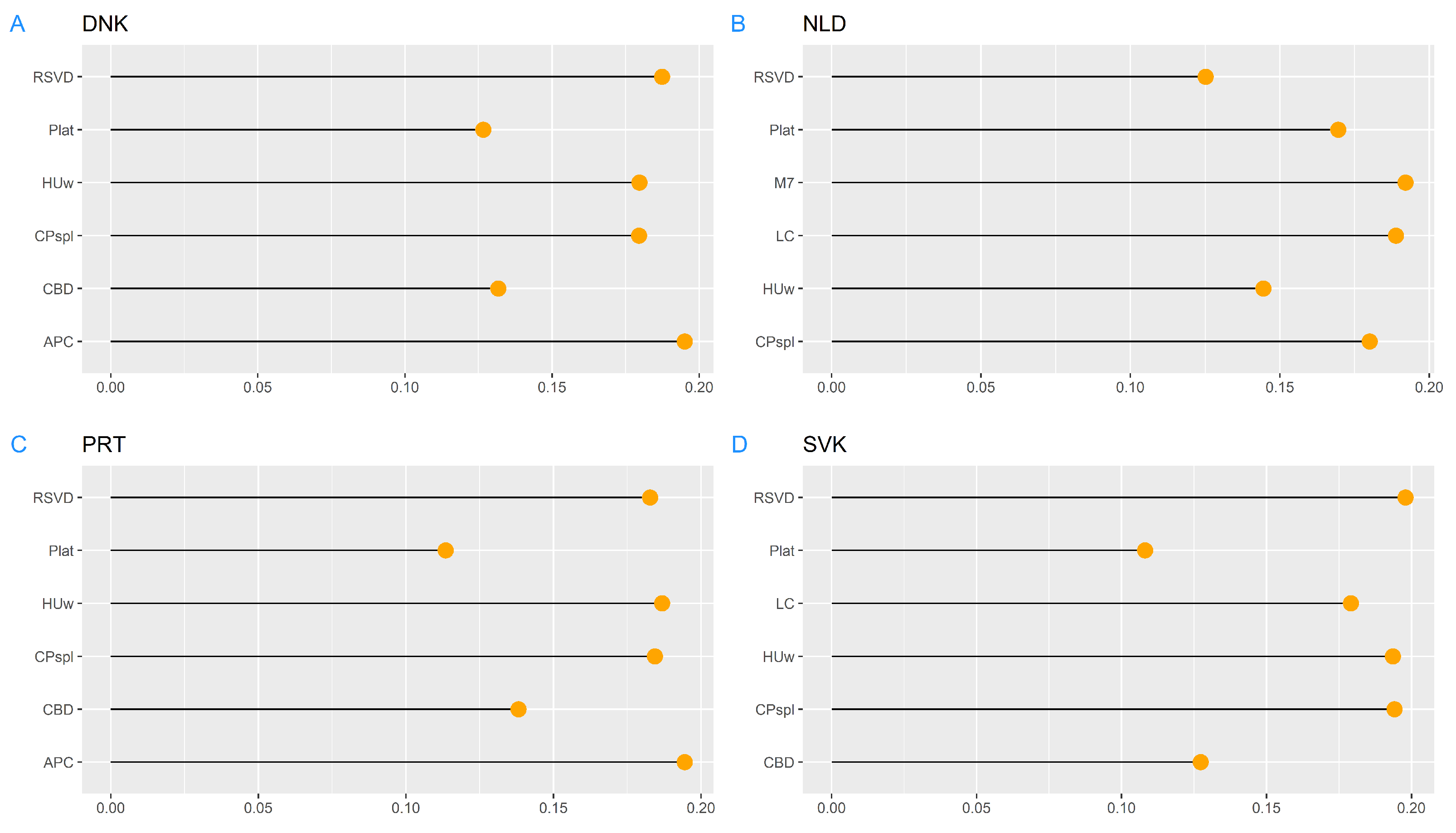
Figure 1. Model confidence set and BME model weights per country, total population. Notes: DNK = Denmark; NLD = The Netherlands; PRT = Portugal; SVK = Slovakia.
Risks 09 00096 g001
Figure 2. NLD: BME forecast of unisex period and cohort life expectancy and pension age along with 95% prediction intervals.
Risks 09 00096 g002
Figure 3. NLD: Expected years in retirement for each sex based on period and cohort projections.
Risks 09 00096 g003
Figure 4. NLD: Legislated retirement age and age with remaining cohort life expectancy equal to the 18.26 years target.
Risks 09 00096 g004
Figure 5. DNK: BME forecast of unisex period and cohort life expectancy and pension age along with 95% prediction intervals.
Risks 09 00096 g005
Figure 6. DNK: Expected years in retirement for each sex based on period and cohort projections.
Risks 09 00096 g006
Figure 7. DNK: Forecast of the legislated retirement age and age with remaining cohort life expectancy equal to the 14.5 years target.
Risks 09 00096 g007
Figure 8. PRT: BME forecast of unisex period and cohort life expectancy and pension age along with 95% prediction intervals.
Risks 09 00096 g008
Figure 9. PRT: Expected years in retirement for each sex based on period and cohort projections.
Risks 09 00096 g009
Figure 10. SVK: BME forecast of unisex period and cohort life expectancy and pension age along with 95% prediction intervals.
Risks 09 00096 g010
Figure 11. SVK: Expected years in retirement for each sex based on period and cohort projections.
Risks 09 00096 g011
Table 1. Analytical structure of the stochastic mortality models used in this study.
ModelModel Structure
LC η x , t = α x + β x ( 1 ) κ t ( 1 )
APC η x , t = α x + κ t ( 1 ) + γ t x
RH η x , t = α x + β x ( 1 ) κ t ( 1 ) + β x ( 0 ) γ t x
CBD η x , t = κ t ( 1 ) + x x ¯ κ t ( 2 )
M7 η x , t = κ t ( 1 ) + x x ¯ κ t ( 2 ) + x x ¯ 2 σ κ t ( 3 ) + γ t x
Plat η x , t = α x + κ t ( 1 ) + x x ¯ κ t ( 2 ) + x ¯ x + κ t ( 3 ) + γ t x
HUw y t x i = f t x i + σ t x i ϵ t , i
CPspl η = B α
RSVD m x , t = j = 1 q d j U j t V j x + ϵ x , t
η x , t denotes the linear predictor; α x and β x ( i ) denote age-specific terms; κ t ( i ) and γ t x are period and cohort indices; y t ( x i ) = l o g ( m x i , t ) ; f t ( x i ) is a continuous and smooth function; σ t ( x i ) is a volatility term; ϵ t , i and ϵ ( x , t ) are error terms; B are B-spline bases with a roughness penalty; α is a vector of parameters.
Table 2. NLD: Forecast of life expectancy and pension age markers.
Year
Longevity Marker/Pension Age20202025(a)203020402050
e 65 , g P ( t ) 20.4220.9321.4122.3723.32
e 65 , g C ( t ) 21.8222.3522.8723.8724.81
e 65 , g G a p ( t ) 1.401.421.461.491.49
x r P ( t ) (b)66.3367.25686970
x r C ( t ) (c)66.3367.2568.570.571.5
x r P ( t ) (d)66.3367.6768.1569.1170.06
x r C ( t ) (e)66.3369.0969.6170.6171.55
x r ( t ) [ e x r , m e n C = 18.26 ] 67.2067.8168.3769.3970.31
x r ( t ) [ e x r , w o m e n C = 18.26 ] 70.3670.8671.3472.2573.11
Expected years in retirement
- Men (b)19.0318.7618.5818.6118.54
- Women (b)21.9221.5421.3021.2521.15
- Men (c)19.0318.7618.1417.2817.20
- Women (c)21.9221.5420.8419.8619.75
Notes: (a) Year when the automatic indexation rule comes into force. Values computed using Equation (5) and: (b) period life expectancy; (c) cohort life expectancy; (d) period or (e) cohort life expectancy but excluding additional provisions capping the maximum increase per period and the indexation lag.
Table 3. DNK: Forecast of life expectancy and pension age markers.
Year
Longevity Marker/Pension Age2020203020402050
e 60 , g P ( t ) 23.8825.0826.1527.16
e 60 , g C ( t ) 25.8727.0128.0429.01
e 60 , g G a p ( t ) 1.991.931.901.85
x r P ( t ) (a)67687071
x r C ( t ) (b)67687072
x r P ( t ) (c)6768.7070.0071.12
x r C ( t ) (d)6770.7571.9673.03
x r ( t ) [ e x r , m e n C = 14.5 ] 71.6472.8873.9674.92
x r ( t ) [ e x r , w o m e n C = 14.5 ] 73.9575.0376.0477.00
Expected years in retirement
- Men (a)18.3318.5417.7617.77
- Women (a)20.5420.6319.7319.70
- Men (b)18.3318.5417.7616.91
- Women (b)20.5420.6319.7318.78
Notes: Values computed using Equation (7) and: (a) period life expectancy; (b) cohort life expectancy; (c) period or (d) cohort life expectancy but excluding additional provisions capping the maximum increase per period and the indexation lag.
Table 4. PRT: Forecast of life expectancy and pension age markers.
Year
Longevity Marker/Pension Age2020203020402050
e 65 , g P ( t ) 20.2521.2222.2323.30
e 65 , g C ( t ) 21.5922.7523.9625.04
e 65 , g G a p ( t ) 1.341.531.731.74
x r P ( t ) (a)66.426767.6768.42
x r C ( t ) (b)66.4267.0867.9268.67
Expected years in retirement
- Men (a)18.2218.7519.1419.39
- Women (a)22.2822.9723.5723.91
- Men (b)18.2218.6818.9219.16
- Women (b)22.2822.8823.3123.65
Notes: Values computed using Equation (8) and: (a) period life expectancy; (b) cohort life expectancy.
Table 5. SVK: Forecast of life expectancy and pension age markers.
Year
Longevity Marker/Pension Age2020203020402050
e 65 , g P ( t ) 18.8019.5920.3521.07
e 65 , g C ( t ) 19.8320.6521.4022.09
e 65 , g G a p ( t ) 1.041.071.061.02
x r P ( t ) (a)62.6763.5364.3065.04
x r C ( t ) (b)62.6763.5564.3465.05
x r ( t ) 2019 Reform62.6764.0064.0064.00
Expected years in retirement
- Men (a)17.9018.1518.4018.59
- Women (a)21.9121.9922.0822.15
- Men (b)17.9018.1418.3718.57
- Women (b)21.9121.9722.0522.13
- Men: 2019 Reform17.9017.8018.6219.39
- Women: 2019 Reform21.9121.5522.3623.12
Notes: Values computed using Equation (11) and: (a) period life expectancy; (b) cohort life expectancy.
Publisher’s Note: MDPI stays neutral with regard to jurisdictional claims in published maps and institutional affiliations.