Ruin Probability for the Insurer–Reinsurer Model for Exponential Claims: A Probabilistic Approach

Abstract

In this paper, we consider a two-dimensional risk process in which the companies split each claim and premium in a fixed proportion. It serves as a classical framework of a quota-share reinsurance contract for a given business line. Such a contract reduces the insurer’s exposure to the liabilities created through its underwriting activities. For the analyzed model, we derive a joint infinite-time ruin probability formula for exponentially distributed claims. To this end, we apply a change of measure technique. We illustrate the admissible range of parameters of the risk process. We also justify our result using Monte Carlo simulations and compare it with Theorem 2 in Avram, Palmowski and Pistorius [Insurance: Mathematics and Economics 42 (2008) 227], which was obtained by explicitly inverting a Laplace transform of the ruin probability. Our formula leads to a correction of that result. Finally, we note that the obtained formula leads to efficient approximation of the ruin probability for other claim amount distributions using De Vylder’s idea.

1. Introduction

Insurance companies have to comply with Solvency II requirements. This framework offers insurers the possibility to improve business strategy and capital allocation. In this context, risk mitigation appears of primary importance. Reinsurance is one of the most important risk mitigation tools used by insurers. An insurer can use it to reduce its insurance risk and the volatility of its financial results. In order to construct and price a reinsurance contract, it is important to examine the risk associated with a portfolio of policies, which mathematically leads to the analysis of the aggregate claim process dynamics.

We focus here on a two-dimensional risk process where the claims are coupled in a specific manner, namely, the claim counting process is the same for both dimensions and the value of each claim is split proportionally between both sides. Formally, we define the considered model on the probability space $(\Omega ,\mathcal{F},\mathrm{P})$ as a system of two Cramér-Lundberg models, which are coupled via a Poisson process and random claims as:

$$\begin{array}{c}\hfill \left(\begin{array}{c}{R}_1\left(t\right)\\ R_2\left(t\right)\end{array}\right)=\left(\begin{array}{c}{u}_1\\ u_2\end{array}\right)+\left(\begin{array}{c}{c}_1\\ c_2\end{array}\right)t-\left(\begin{array}{c}a\\ 1-a\end{array}\right){\displaystyle \sum _{k=1}^{N\left(t\right)}}{X}_k.\end{array}$$

(1)

where $(u_1,u_2)$ denote initial capital, $(c_1,c_2)$ are the premium income rates, and $N\left(t\right)$ is a claim counting Poisson process with intensity $\lambda >0$ independent of the claim amounts ${\left\{X_i\right\}}_{i\ge 1}$, which form a sequence of independent and identically distributed positive random variables with common mean $\mu =\mathrm{E}\left(X_k\right)<\infty$. The parameter $a\in [0;1]$ defines the split proportions a and $1-a$ of each claim between the processes $R_1\left(t\right)$ and $R_2\left(t\right)$, respectively.

The presented two-dimensional model classically describes the situation of insurance and reinsurance companies with the proportional quota-share reinsurance contract for one business line. The model was introduced in Avram et al. (2008b) and Avram et al. (2008a). It induces a specific strong dependence between the two risk processes $R_1\left(t\right)$ and $R_2\left(t\right)$. Another type of dependence was studied in Behme et al. (2020), where the link of the components of the process was established by a random bipartite network. An extension to a system of two insurers was introduced by Badescu et al. (2011), where the first insurer is subject to claims arising from two independent compound Poisson processes and the second insurer covers a proportion of the claims arising from one of these two compound Poisson processes. A similar two-dimensional model, where both claims and pure premiums are split between the two companies, was considered by Ji and Robert (2018) but with a fractional Brownian motion as driving aggregate loss amount process, whereas Michna (2020) investigated a model driven by a general spectrally positive or negative Lévy process, see also Avram et al. (2008b).

Next, we assume that

$$\begin{array}{cc}\hfill c_1& =(1+{\theta }_1)a\lambda \mathrm{E}\left(X_k\right),\hfill \\ \hfill c_2& =(1+{\theta }_2)(1-a)\lambda \mathrm{E}\left(X_k\right),\hfill \end{array}$$

(2)

where ${\theta }_1,{\theta }_2>0$ are the relative safety loadings for the two companies. Let us treat the second company as the reinsurer. Hence, due to the higher acquisition and administration costs of the insurer, it is natural to assume that the premium rate for the insurer is higher than for the reinsurer and therefore the following relation holds: ${\theta }_1>{\theta }_2$.

Our main goal was to obtain an analytical expression for the joint ruin probability in the infinite time horizon, which is formally defined as:

$$\psi (u_1,u_2)=\mathrm{P}(\tau (u_1,u_2)<\infty ),$$

(3)

where $\tau (u_1,u_2)$ is the ruin time that at least one of the companies is ruined:

$$\tau (u_1,u_2)=inf\{t\ge 0:R_1\left(t\right)<0\vee R_2\left(t\right)<0\}.$$

(4)

We investigated the two-dimensional risk process given by Equation (1) with claims described by the exponential distribution.

The rest of this paper is structured as follows: In Section 2, we present a probabilistic approach to the ruin probability problem for the insurer–reinsurer model. We derive an analytical result for the ruin probability using purely probabilistic arguments. Our result leads to a correction of Theorem 2 in Avram et al. (2008a), which was obtained with the use of the double Laplace transform inversion technique. To the best of our knowledge, in the literature, there are no other explicit solutions for the exact ruin probability in the infinite time horizon for the model considered here. The obtained results are discussed and compared with the corrected Theorem 2 and Monte Carlo method approximations. Concluding remarks are formulated in Section 3.

2. Ruin Probability: A Probabilistic Approach

In this section, we present the main analytical results devoted to the problem of the joint ruin probability of the two-dimensional risk process given by (1). Firstly, we recall certain geometric properties of the considered model that were presented in Avram et al. (2008a), which allow us to reduce the complexity of the problem. Secondly, using stochastic arguments, we derive an explicit analytical solution for the ruin probability (3) for claims following the exponential law. Finally, taking advantage of the numerical experiments available for our solution together with Monte Carlo simulations, we correct the result presented in Avram et al. (2008a).

2.1. Problem Reduction

Let us observe that due to the specific construction of the considered two-dimensional risk process, in which we assume that each claim is split between the insurer and reinsurer with the proportions a and $1-a$, respectively, the two-dimensional problem can be reduced to the one-dimensional (cf. Avram et al. (2008a)). First, let us notice that the ruin probability of the system $(R_1\left(t\right),R_2\left(t\right))$ is equal to the ruin probability of the system $\left(R_1\left(t\right)/a,R_2\left(t\right)/(1-a)\right)$:

$$\begin{array}{c}\hfill \left(\begin{array}{c}{R}_1\left(t\right)/a\\ R_2\left(t\right)/(1-a)\end{array}\right)=\left(\begin{array}{c}{u}_1/a\\ u_2/(1-a)\end{array}\right)+\left(\begin{array}{c}(1+{\theta }_1)\lambda \mathrm{E}\left(X_k\right)\\ (1+{\theta }_2)\lambda \mathrm{E}\left(X_k\right)\end{array}\right)t-{\displaystyle \sum _{k=1}^{N\left(t\right)}}{X}_k.\end{array}$$

(5)

We now distinguish between the two cases:

(i)

$u_1/a\ge u_2/(1-a)$ and

(ii)

$u_1/a<u_2/(1-a)$.

Observe that for (i) each trajectory of the process, $R_1\left(t\right)/a$ is above the corresponding trajectory of the process $R_2\left(t\right)/(1-a)$; therefore, the here-considered joint ruin event (4) occurs only when the ruin happens for the process $R_2\left(t\right)$ and consequently

$$\psi (u_1,u_2)=\mathrm{P}(inf\{t\ge 0:R_2\left(t\right)<0\}<\infty ).$$

(6)

Clearly, that observation reduces the two-dimensional case to the purely one-dimensional problem with exponential claims for which the the formula is well-known in the literature (see, e.g., Asmussen and Albrecher (2010); Rolski et al. (1999)).

For (ii), there exists a time point $T>0$ before which the ruin of process (1) can be triggered by the insurer; after this point, it can only be triggerd by the reinsurer. This is a solution of the equation: $u_1/a+(1+{\theta }_1)\lambda \mathrm{E}\left(X_k\right)t=u_2/(1-a)+(1+{\theta }_2)\lambda \mathrm{E}\left(X_k\right)t$. Hence,

$$\begin{array}{c}\hfill T=\frac{u_1/a-u_2/(1-a)}{({\theta }_2-{\theta }_1)\lambda \mathrm{E}\left(X_k\right)}.\end{array}$$

(7)

Then, we can verify that for any $t\in [0,T]$, the relation $R_2\left(t\right)/(1-a)\ge R_1\left(t\right)/a$ holds; for $t>T$, the opposite is true. This asserts that for (ii), the two-dimensional problem can also be reduced to the one-dimensional case. Namely, using the Markovian property of the system, we formulate the problem in the following way. Observe that non-ruin in the infinite time horizon is equivalent to the event where the insurer will avoid ruin up to time T, ending with some positive capital, which will be the initial capital for the reinsurer, and then the reinsurer will never go bankrupt. This allows us to write the following equation, which was also presented in Avram et al. (2008a):

$$\begin{array}{c}\hfill \psi (u_1,u_2)=1-{\int }_0^{\infty }(1-{\psi }_2\left(z\right)){\mathrm{P}}_{(u_1,T)}\left(\mathrm{d}z\right),\end{array}$$

(8)

where ${\psi }_2\left(z\right)$ is the ruin probability in infinite time for the reinsurer and

$$\begin{array}{c}\hfill {\mathrm{P}}_{(u_1,T)}\left(\mathrm{d}z\right)=\mathrm{P}\left({\displaystyle \underset{s\le T}{inf}}{R}_1\left(s\right)/a>0,R_1\left(T\right)/a\in \mathrm{d}z|R_1\left(0\right)=u_1\right)\end{array}$$

(9)

denotes the joint probability that the insurer avoids ruin until T and reaches the level z.

Equation (8) can be rewritten as

$$\begin{array}{c}\hfill \psi (u_1,u_2)=1-\mathrm{P}\left({\displaystyle \underset{s\le T}{inf}}{R}_1\left(s\right)/a>0\right)+{\int }_0^{\infty }{\psi }_2\left(z\right){\mathrm{P}}_{(u_1,T)}\left(\mathrm{d}z\right).\end{array}$$

(10)

In the next part of this work, we derive analytical formulas for the ruin probability considered here using Formula (10) for claims distributed according to the exponential law.

2.2. Ruin Probability for Exponential Claims

If the claims for the insurer–reinsurer model given in Equation (1) are exponentially distributed, then the ruin probability defined in Equation (10) can be given explicitly. Taking advantage of the elementary formula for the ruin probability ${\psi }_2\left(z\right)$ for the exponential distribution, we can reduce the integral in (10) to a quantity that is proportional (up to some deterministic factor) to the probability of ruin for the Cramér-Lundberg model in finite time. The following theorem presents the final form of the joint ruin probability formula for the two-dimensional risk process with exponential claims.

Theorem 1.

Let ${\theta }_1>{\theta }_2$, and $X_k$ be exponentially distributed with mean ${\beta }^{-1}$. Then, if ${\theta }_1>{(1+{\theta }_2)}^2-1$, the joint ruin probability specified in Equation (10) of the risk process defined in Equation (1) has the following form:

$$\begin{array}{c}\hfill \psi (u_1,u_2)=\left\{\begin{array}{cc}\frac{1}{1+{\theta }_2}\exp \left(-\frac{\gamma u_2}{1-a}\right)\hfill & \mathrm{for}\left(i\right),\hfill \\ r(\lambda ,\beta ,{\theta }_1,u_1/a,T)+\frac{1}{1+{\theta }_2}\exp \left(-\gamma u_1/a-\varphi \left(\gamma \right)T\right)\{1-\hfill \\ r(\lambda \beta /(\beta -\gamma ),\beta -\gamma ,(1+{\theta }_1){\left(\beta -\gamma \right)}^2/{\beta }^2-1,u_1/a,T)\}\hfill & \mathrm{for}\left(ii\right),\hfill \end{array}\right.\end{array}$$

where $\gamma =\frac{{\theta }_2\beta }{1+{\theta }_2}$, $\varphi \left(s\right)=(1+{\theta }_1)\frac{\lambda }{\beta }s-\lambda \left(\frac{\beta }{\beta -s}-1\right)$ and

$$\begin{array}{cc}\hfill & r(\lambda ,\beta ,\theta ,u,T)=\frac{1}{1+\theta }\exp \left(-\frac{\theta \beta u}{1+\theta }\right)-\frac{1}{\pi }{\int }_0^{\pi }\frac{f_1\left(x\right)f_2\left(x\right)}{f_3\left(x\right)}\mathrm{d}x\hfill \end{array}$$

(11)

with

$$\begin{array}{c}{f}_1\left(x\right)=f_1(x,\lambda ,\theta ,u,T)=\frac{1}{1+\theta }\exp \left(2T\sqrt{1+\theta }\lambda \cos \left(x\right)\right)\hfill \\ \times \exp \left\{-(2+\theta )\lambda T+u\beta \left(\cos \left(x\right)/\sqrt{1+\theta }-1\right)\right\},\end{array}$$

(12)

$$\begin{array}{c}\hfill f_2\left(x\right)=f_2(x,\beta ,\theta ,u)=\cos \left(\beta u\sin \left(x\right)/\sqrt{1+\theta }\right)-\cos \left(\beta u\sin \left(x\right)/\sqrt{1+\theta }+2x\right),\end{array}$$

(13)

$$\begin{array}{c}{f}_3\left(x\right)=f_3(x,\theta )=\frac{2+\theta }{1+\theta }-2\cos \left(x\right)/\sqrt{1+\theta }.\end{array}$$

(14)

Proof. 

First, for case (i), as discussed in Section 2.1, the ruin probability for the two-dimensional model simplifies to the one-dimensional problem for the reinsurer risk process with claims exponentially distributed with mean $(1-a)/\beta$, the intensity of the Poisson process $\lambda$, and initial capital $u_2$. Therefore, the result for this part follows directly from the well-known formula for the ruin probability in infinite time Asmussen and Albrecher (2010).

Second, for case (ii), the first factor $1-\mathrm{P}({\displaystyle {inf}_{s\le T}}{R}_1\left(s\right)/a>0)$ in Formula (10) is a ruin probability for the process $R_1\left(t\right)/a$ in the finite time interval $[0,T]$ and its explicit form is known, see Asmussen (1984), with several misprints pointed out by Barndorff-Nielsen and Schmidli (1995), see also Asmussen and Albrecher (2010); Burnecki and Teuerle (2011). By combining that formula and the known formula for the ruin probability in infinite time ${\psi }_2\left(z\right)$, we obtain the following expression:

$$\begin{array}{c}\hfill \psi (u_1,u_2)=r(\lambda ,\beta ,{\theta }_1,u_1/a,T)+\frac{1}{1+{\theta }_2}{\int }_0^{\infty }exp\left(-\frac{{\theta }_2\beta z}{1+{\theta }_2}\right){\mathrm{P}}_{(u_1,T)}\left(\mathrm{d}z\right),\end{array}$$

(15)

where $r(\lambda ,\beta ,\theta ,u,T)$ corresponds to the ruin probability in finite time T of the one-dimensional risk process with initial capital u, safety loading $\theta$, Poisson arrival intensity $\lambda$, and exponential claims with mean $1/\beta$, and has the following form (see Asmussen and Albrecher (2010)):

$$\begin{array}{c}r(\lambda ,\beta ,\theta ,u,T)=\frac{1}{1+\theta }\exp \left(-\frac{\theta \beta u}{1+\theta }\right)-\frac{1}{\pi }{\int }_0^{\pi }\frac{f_1\left(x\right)f_2\left(x\right)}{f_3\left(x\right)}\mathrm{d}x\end{array}$$

(16)

with $f_1\left(x\right)=f_1(x,\lambda ,\theta ,u,T)$, $f_2\left(x\right)=f_2(x,\beta ,\theta ,u)$ and $f_3\left(x\right)=f_3(x,\theta )$ as in Equations (12)–(14).

The integral in Equations (10) and (15) can be rewritten (up to a constant) as

$$\begin{array}{c}\hfill {\int }_0^{\infty }\exp \left(-\gamma z\right){\mathrm{P}}_{(u_1,T)}\left(\mathrm{d}z\right),\end{array}$$

(17)

and can be interpreted, see Formula (9), as the Laplace transform of the random variable $R_1\left(T\right)/a$ at point $\gamma$, given the process $R_1\left(t\right)$ is non-negative up to the time point T and $R_1\left(0\right)=u_1$; namely, we obtain

$$\begin{array}{c}\hfill \mathrm{E}\left(\exp \left(-\gamma R_1\left(T\right)/a\right),{\displaystyle \underset{s\le T}{inf}}{R}_1\left(s\right)/a>0|R_1\left(0\right)=u_1\right).\end{array}$$

(18)

The process $R_1\left(t\right)/a$ is a standard Cramér–Lundberg process with initial capital $u_1/a$, safety loading ${\theta }_1$, Poisson process with intensity $\lambda$, and exponential claims with mean ${\beta }^{-1}$. Therefore, the Laplace transform (18) is equal to:

$$\begin{array}{cc}\hfill & \mathrm{E}\left(\exp \left(-\gamma R_1\left(T\right)/a\right),{\displaystyle \underset{s\le T}{inf}}{R}_1\left(s\right)/a>0|R_1\left(0\right)=u_1\right)=\hfill \\ & =\exp (-\gamma u_1/a)\mathrm{E}[\exp \left\{-\gamma \left((1+{\theta }_1)\frac{\lambda }{\beta }T-{\displaystyle \sum _{i=1}^{N\left(T\right)}}{X}_i\right)\right\},\hfill \\ & {\displaystyle \underset{s\le T}{inf}}{R}_1\left(s\right)/a>0|R_1\left(0\right)=u_1].\hfill \end{array}$$

(19)

In the next step, we introduce the following change in measure with respect to natural filtration ${\left({\mathcal{F}}_t\right)}_{t\ge 0}$ generated by the process $R_1\left(t\right)$:

$${\displaystyle \begin{array}{c}\mathbb{Q}\left(A\right)=\hfill \\ ={\int }_A\exp \left\{-\gamma \left((1+{\theta }_1)\frac{\lambda }{\beta }T-{\displaystyle \sum _{i=1}^{N\left(T\right)}}{X}_i\right)+\varphi \left(\gamma \right)T\right\}\mathrm{d}\mathbb{P},\mathrm{for}A\in {\mathcal{F}}_T,\hfill \end{array}}$$

(20)

where $\mathbb{P}$ denotes the measure on the natural filtration generated by the process $R_1\left(t\right)$ and $\mathbb{Q}$ denotes the new measure. Now, we are able to write Equation (19) as:

$$\begin{array}{cc}\hfill & \exp (-\gamma u_1/a)\mathrm{E}\left[\exp \left\{-\gamma \left((1+{\theta }_1)\frac{\lambda }{\beta }T-{\displaystyle \sum _{i=1}^{N\left(T\right)}}{X}_i\right)+\varphi \left(\gamma \right)T-\varphi \left(\gamma \right)T\right\},\right.\hfill \\ \hfill & \left.{\displaystyle \underset{s\le T}{inf}}{R}_1\left(s\right)/a>0|R_1\left(0\right)=u_1\right]=\exp \left\{-\gamma u_1/a-\varphi \left(\gamma \right)T\right\}\hfill \\ & \times {\mathrm{E}}_{\mathbb{Q}}\left(1;{\displaystyle \underset{s\le T}{inf}}{R}_1\left(s\right)/a>0|R_1\left(0\right)=u_1\right)=\hfill \\ & =\exp \left\{-\gamma u_1/a-\varphi \left(\gamma \right)T\right\}\mathbb{Q}\left({\displaystyle \underset{s\le T}{inf}}{R}_1\left(s\right)/a>0|R_1\left(0\right)=u_1\right).\hfill \end{array}$$

(21)

Now observe that the process $R_1\left(t\right)$ under the new measure $\mathbb{Q}$ is also a Cramér–Lundberg process but with a modified intensity and claim amount distribution. To see this, let us calculate the moment generating function of $(1+{\theta }_1)\frac{\lambda }{\beta }t-{\sum }_{i=1}^{N\left(t\right)}{X}_i$ under the new measure $\mathbb{Q}$:

$$\begin{array}{cc}\hfill & \mathcal{L}\left(s\right)={\mathrm{E}}_{\mathbb{Q}}\left[\exp \left\{s\left((1+{\theta }_1)\frac{\lambda }{\beta }t-{\displaystyle \sum _{i=1}^{N\left(t\right)}}{X}_i\right)\right\}\right]\hfill \\ \hfill & =\mathrm{E}\left[\exp \left\{s\left((1+{\theta }_1)\frac{\lambda }{\beta }t-{\displaystyle \sum _{i=1}^{N\left(t\right)}}{X}_i\right)-\gamma \left((1+{\theta }_1)\frac{\lambda }{\beta }t-{\displaystyle \sum _{i=1}^{N\left(t\right)}}{X}_i\right)+\varphi \left(\gamma \right)t\right\}\right]\hfill \\ \hfill & =\mathrm{E}\left[\exp \left\{(s-\gamma )\left((1+{\theta }_1)\frac{\lambda }{\beta }t-{\displaystyle \sum _{i=1}^{N\left(t\right)}}{X}_i\right)+\varphi \left(\gamma \right)t\right\}\right]\hfill \\ \hfill & \stackrel{*}{=}\exp \left\{(s-\gamma )(1+{\theta }_1)\frac{\lambda }{\beta }t+\lambda t\left(\frac{\beta }{\beta -\gamma +s}-1\right)+\gamma (1+{\theta }_1)\frac{\lambda }{\beta }t-\lambda t\left(\frac{\beta }{\beta -\gamma }-1\right)\right\}\hfill \\ \hfill & =\exp \left\{(1+{\theta }_1)\frac{\lambda }{\beta }st+\lambda t\left(\frac{\beta }{\beta -\gamma +s}-1\right)-\lambda t\left(\frac{\beta }{\beta -\gamma }-1\right)\right\}\hfill \\ \hfill & =\exp \left\{(1+{\theta }_1)\frac{\lambda }{\beta }st+\frac{\lambda \beta }{\beta -\gamma }t\left(\frac{\beta -\gamma }{\beta -\gamma +s}-1\right)\right\},\hfill \end{array}$$

(22)

where the equality $\stackrel{*}{=}$ follows from the moment-generating function of the process $(1+{\theta }_1)\frac{\lambda }{\beta }t-{\sum }_{i=1}^{N\left(t\right)}{X}_i$ under the natural measure having the following form:

$$\begin{array}{c}\hfill \mathrm{E}\left[\exp \left\{s\left((1+{\theta }_1)\frac{\lambda }{\beta }t-{\displaystyle \sum _{i=1}^{N\left(t\right)}}{X}_i\right)\right\}\right]=(1+{\theta }_1)\frac{\lambda }{\beta }st+\lambda t\left(\frac{\beta }{\beta +s}-1\right).\end{array}$$

(23)

By comparing the final form of Equation (22) and the moment-generating function transform of the original model (23), we deduce that after the change in measure, the process $R_1\left(t\right)/a$ is a Cramér–Lundberg process with initial capital $u_1/a$, safety loading $(1+{\theta }_1){\left(\beta -\gamma \right)}^2/{\beta }^2-1$ (which is positive based on the assumptions), Poisson process with intensity $\lambda \beta /(\beta -\gamma )$, and claims $X_i$, which are exponentially distributed with mean ${(\beta -\gamma )}^{-1}$.

Since the new safety loading is positive, we can apply the finite-time ruin probability for the exponential claims and obtain

$$\begin{array}{cc}\hfill & \mathrm{E}\left(\exp (-\gamma R_1\left(T\right)/a),{\displaystyle \underset{s\le T}{inf}}{R}_1\left(s\right)/a>0|R_1\left(0\right)=u_1\right)=\exp \left(-\gamma u_1/a-\varphi \left(\gamma \right)T\right)\hfill \\ & \times \left\{1-r\left(\lambda \beta /(\beta -\gamma ),\beta -\gamma ,(1+{\theta }_1){\left(\beta -\gamma \right)}^2/{\beta }^2-1,u_1/a,T\right)\right\}.\hfill \end{array}$$

(24)

Finally, for case (ii), we have

$$\begin{array}{cc}\hfill & \psi (u_1,u_2)=r(\lambda ,\beta ,{\theta }_1,u_1/a,T)+\frac{1}{1+{\theta }_2}\exp (-\gamma u_1/a-\varphi \left(\gamma \right)T)\hfill \\ \hfill & \left(1-r\left(\lambda \beta /(\beta -\gamma ),\beta -\gamma ,(1+{\theta }_1){\left(\beta -\gamma \right)}^2/{\beta }^2-1,u_1/a,T\right)\right),\hfill \end{array}$$

(25)

which concludes the proof. □

Finally, let us comment on the assumption that was made at the beginning of our considerations: ${\theta }_1>{\theta }_2$. We note that the case ${\theta }_1<{\theta }_2$ can be treated as equivalent to the problem of calculating the ruin probability for $R_1$ being a reinsurer and $R_2$ being an insurer (the processes swap their roles and the probabilistic approach can be repeated). If the safety loadings are equal, the situation becomes trivial; namely, after dividing the process $R_1$ by a and $R_2$ by $1-a$, the trajectories differ only by a constant, so the joint ruin probability reduces to the ruin probability of the lower process.

2.3. Comparison with Other Results

The formula for the ruin probability presented in Theorem 1 in case (ii) is consistent with the results obtained for the spectrally negative Lévy process in Avram et al. (2008b), where a similar two-dimensional system was considered but there was no closed-form formula for the exponential claims. Our result is simple to use and therefore might be easily used in applications and in approximations of ruin probabilities for models with general claim amount distributions, see Burnecki et al. (2019).

Our result corresponds to the second case of Theorem 2 in Avram et al. (2008a), which was obtained by the inversion of the double Laplace transform. However, in that work, limits of the integral in the final formula should be inverted (this mistake is present throughout the text). This leads to the following corrected formulation of the second case of Theorem 2:

$$\begin{array}{cc}\hfill \psi \left(u_1,u_2\right)& =\frac{a\beta }{1+{\theta }_1}{e}^{-\frac{{\theta }_1\beta u_1}{a(1+{\theta }_1)}}+\frac{(1-a)\beta }{1+{\theta }_2}{e}^{-\frac{{\theta }_2\beta u_2}{(1-a)(1+{\theta }_2)}}\hfill \\ \hfill & -\frac{1+{\theta }_1}{1+{\theta }_2}{e}^{-\frac{\beta ({\theta }_1-2{\theta }_2-{\theta }_2^2)u_1}{a(1+{\theta }_1)(1+{\theta }_2)}-\frac{{\theta }_2\beta u_2}{(1-a)(1+{\theta }_2)}}-\omega \left(x_1,x_2\right),\hfill \end{array}$$

(26)

where

$$\omega (x_1,x_2)=\frac{p_2-\rho }{\pi }{\int }_{q_{-}}^{q_{+}}{e}^{x_{1}c\left(q\right)+x_{2}q}\frac{f\left(q\right)\sin \left(b\left(q\right)x_1\right)+b\left(q\right)\cos \left(b\left(q\right)x_1\right)}{q(q{p}_2+\beta p_2-\lambda )}dq,$$

$q\pm =-\frac{1}{p_1-p_2}(\sqrt{\lambda }\pm \sqrt{p_1\beta })$, $f\left(q\right)=\beta +q+c\left(q\right)$, $c\left(q\right)=\frac{-(p_1\beta -\lambda +p_{2}q+p_{1}q)}{2p_1}$,

$b\left(q\right)=\frac{\sqrt{4p_1(p_{2}q\beta +p_2{q}^2-\lambda q)-{(p_1\beta -\lambda +p_{2}q+p_{1}q)}^2}}{2p_1}$, $p_1=(1+{\theta }_1)\lambda /\beta$, $p_2=(1+{\theta }_2)\lambda /\beta$ and $\rho =\lambda /\beta$.

In the work of Badescu et al. (2011), a more general model than (1) was investigated. It allows, in addition to the insurer–reinsurer quota share mechanism, another source of claims for the insurer, which was modeled by an independent compound Poisson process with an arbitrary claim size distribution. Nevertheless, the obtained results seem to be less numerically tractable.

Finally, a similar ruin probability problem was discussed by Foss et al. (2017), where the initial reserves of both companies tended to infinity and the generic claim size was heavy-tailed, namely, subexponential.

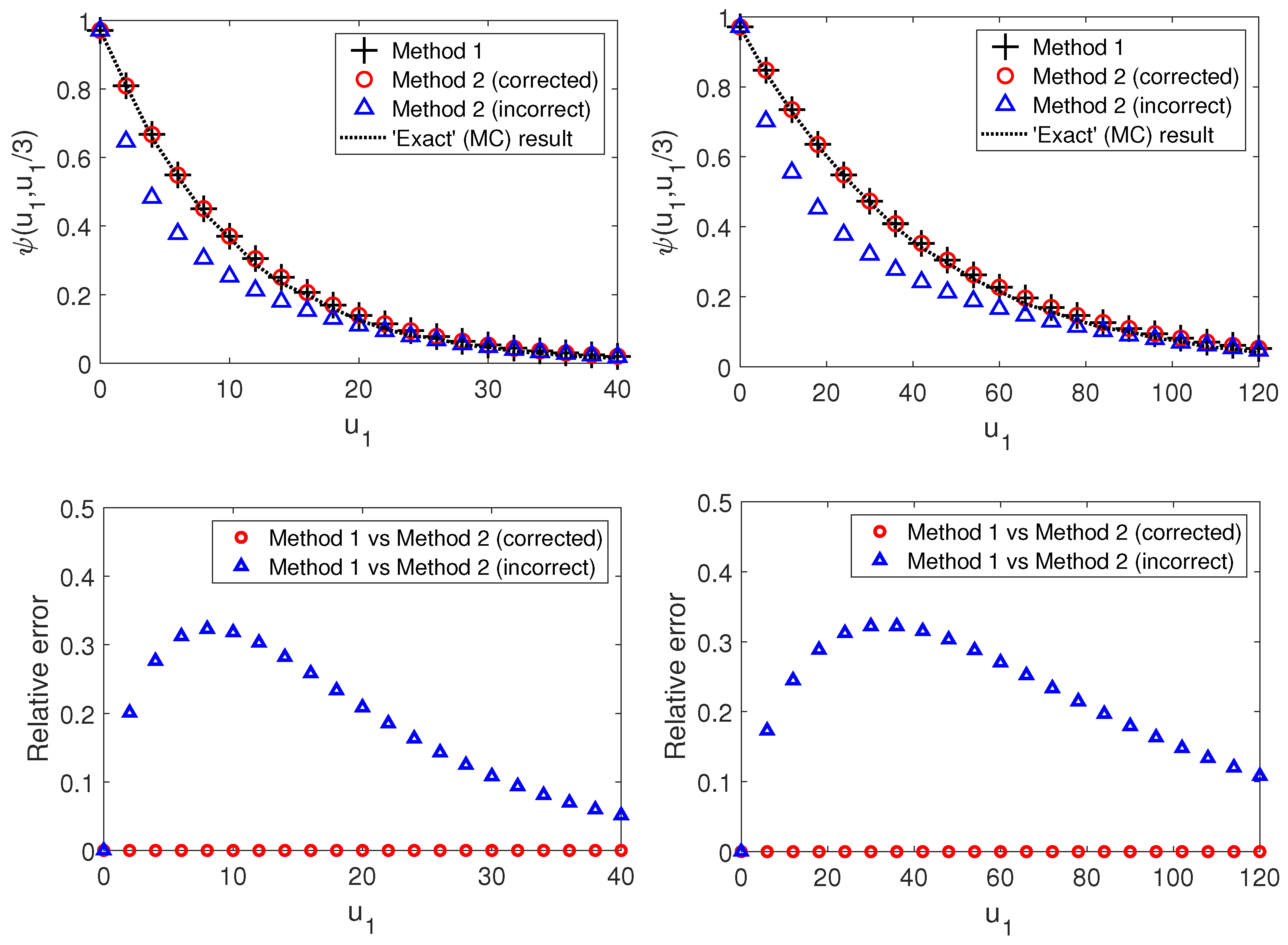
In Figure 1, we illustrate that both formulas, Equation (11) of Theorem 1 and the corrected version of the second case of Theorem 2 of Avram et al. (2008a) given by Formula (26), lead to the same results for the ruin probability (3) of the insurer–reinsurer model (1). Moreover, they coincide with the results obtained by Monte Carlo simulations for the finite time with a sufficiently long horizon. We also show that the original version of Theorem 2 of Avram et al. (2008a) leads to significant relative errors with a maximum around 30% (see both bottom panels). This also confirms the relevance of our findings.

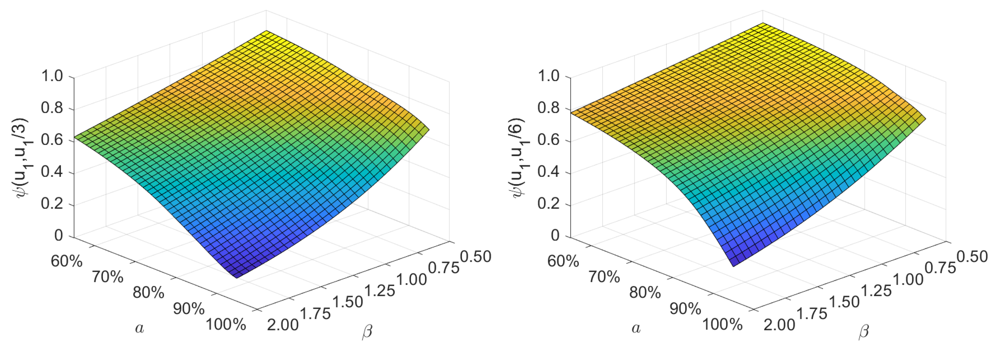
We also performed a numerical analysis in which we checked how the joint ruin probability of the insurer–reinsurer model is affected by the change in selected model parameters’ values. The results presented in Figure 2 were obtained for the insurer–reinsurer model using Theorem 1 with $u_1=10$, ${\theta }_1=10\%$, ${\theta }_2=3\%$, and $\lambda =10$ for various values of the $\beta$ parameter of the exponential claim amount random variable, $\beta \in (0.5,2)$, and for various values of the a parameter of the quota-share contract proportion, $a\in (55\%,95\%)$. Moreover, the analysis was performed for two initial capitals of the reinsurer: in the left panel of Figure 2, we have $u_2=u_1/3$, while in the right panel, it is $u_2=u_1/6$. We can observe that despite the different values of the reinsurer’s initial capital, the considered ruin probability decreases as the mean $1/\beta$ decreases, and increases as the quota-share’s proportion parameter of the insurer a decreases. The lower initial capital of the reinsurer results in (generally) lower values of the ruin probability (3) in the considered parameter space $a\times \beta \in (55\%,95\%)\times (0.5,2)$.

Figure 3 illustrates the values of safety loadings $({\theta }_1,{\theta }_2)$ that fulfil the assumption of Theorem 1: ${\theta }_1>{(1+{\theta }_2)}^2-1$. This corresponds to the second case of Theorem 2 in Avram et al. (2008a). To the best of our knowledge, an analogue of the first case of Theorem 2, namely, a result for the region ${\theta }_1\le {(1+{\theta }_2)}^2-1$, cannot be obtained with the use of the probabilistic approach presented in this work. This is due to, in this case, the change in measure presented in the proof of Theorem 1 not leading to a proper Cramér–Lundberg model. Namely, when ${\theta }_1>{(1+{\theta }_2)}^2-1$, after the change in measure, the safety loading of the model is $(1+{\theta }_1){\left(\beta -\gamma \right)}^2/{\beta }^2-1$, which is negative; therefore, the result for the ruin probability in finite time horizon in (15) cannot be used.

3. Conclusions

In this study, we investigated the problem of ruin probability for a special case of the two-dimensional Cramér–Lundberg risk process. In the considered model, we assumed that both premiums and claims are divided between two lines in fixed proportions. Such a model can describe the evolution of the capital of an insurer and a reinsurer under a proportional reinsurance treaty, which is common in non-life insurance practice. We obtained an explicit ruin probability formula for the considered two-dimensional risk process with claims following the exponential law.

In contrast with the results of Avram et al. (2008a), our main findings were derived using purely stochastic arguments using the change in measure technique. The change in the measure led to a modified two-dimensional Cramér–Lundberg risk process with exponential claims. We also corrected the main result of Avram et al. (2008a) and compared it with our formula using Monte Carlo simulations. All results matched very well.

Finally, we note that the main result of this paper was already applied by Burnecki et al. (2019) to introduce a De Vylder type of approximation of the joint ruin probability for the insurer–reinsurer model for general claim amount distributions having the third finite moment. The approximation was found to be effective, which shows the practical significance of our findings.