Clustering-Based Extensions of the Common Age Effect Multi-Population Mortality Model

Abstract

We introduce four variants of the common age effect model proposed by Kleinow, which describes the mortality rates of multiple populations. Our model extensions are based on the assumption of multiple common age effects, each of which is shared only by a subgroup of all considered populations. This makes the models more realistic while still keeping them as parsimonious as possible, improving the goodness of fit. We apply different clustering methods to identify suitable subgroups. Some of the algorithms are borrowed from the unsupervised learning literature, while others are more domain-specific. In particular, we propose and investigate a new model with fuzzy clustering, in which each population’s individual age effect is a linear combination of a small number of age effects. Due to their good interpretability, our clustering-based models also allow some insights in the historical mortality dynamics of the populations. Numerical results and graphical illustrations of the considered models and their performance in-sample as well as out-of-sample are provided.

1. Introduction

All over the world, progress in medical research, technological developments and a general improvement of living conditions have lead to a steady decrease of mortality during the past century. While this development has several obvious benefits for society and individuals, it also poses a serious financial risk for many stakeholders (see Oppers et al. 2012). This so-called longevity risk consists of an underestimation of future longevity and a resulting lack of assets to meet the liabilities that come with aging populations. In fact, in recent decades, longevity forecasts have been consistently too low, and the potential total size of the global market for longevity risk has been estimated to be trillions of dollars (see Zugic et al. 2010).

One way of addressing longevity risk is to model future mortality stochastically, which is conceptually motivated by empirical observations (see Cairns et al. 2006). Stochastic mortality models have the advantage that they not only provide point forecasts but also allow an estimation of forecast uncertainty and tail risk, and they offer the possibility to easily simulate mortality scenarios. While, initially, such models were used to describe only one population, there are various situations in which it is useful or even necessary to model the mortality of multiple populations simultaneously, see for example Kleinow and Cairns (2013), Cairns (2014) and Chen et al. (2015).

In this paper, we consider an established multi-population mortality model, the common age effect (CAE) model of Kleinow (2015). Its eponymous assumption is that the age effect, the influence of general mortality improvements over time on different ages, is identical or at least similar for all considered populations. This is justified if all these populations exhibit similar age structure, socio-economic characteristics, geographical location and life style factors. However, for arbitrary sets of populations, the assumption is too strong and might only hold on multiple smaller groups or clusters of populations. The benefits of applying clustering methods to heterogeneous mortality data have already been recognized by Hatzopoulos and Haberman (2013), Debón et al. (2017) and Guibert et al. (2020), whose approaches we describe below. Further applications of cluster analysis in mortality modeling are presented by Danesi et al. (2015), who cluster period effects which describe the general mortality development over time instead of age effects, by Léger and Mazzuco (2020), who apply functional cluster analysis to identify groups of populations with similar age distributions of death, and by Wen et al. (2020), who consider groups of Canadian pensioners by pension level and find that clustering can reduce noise in small population data.

In contrast to most of these papers, we focus on age effects instead of period effects or death rates. Additionally, we employ cluster analysis not only as a tool for analyzing the data but also as an essential ingredient for modeling, which takes the possible heterogeneity of populations into account. For this purpose, we present several clustering algorithms, embed them into the CAE model and check their performance in an empirical study. Some of the clustering techniques we use are well-known from the general unsupervised learning literature. In particular, we employ k-means clustering and hierarchical clustering (see Hastie et al. 2017, chapter 14). The latter is at the core of a likelihood-ratio based clustering algorithm we propose, which additionally includes a simple statistical test for checking whether any two populations have the same age effect.

Another clustering algorithm we investigate is more domain-specific: We review the fitting method of the augmented common factor model by Li and Lee (2005) and demonstrate that it yields a grouping of the populations as a by-product in our formulation. Guibert et al. (2020) propose a different clustering-based variant of the Li and Lee (2005) model. They mention two simple clustering methods—expert judgment and hierarchical clustering of period effects—but their focus is not on the investigation of clustering methods but rather on the implications of using such a clustering-based mortality model for risk management.

Finally, we propose a new model related to the CAE model, which to the best of our knowledge has not been investigated before. For the calibration of this model, we combine ideas from fuzzy clustering with maximum likelihood estimation and refer to this method as fuzzy maximum likelihood clustering. While in the CAE model a number of populations share a common age effect, this is in general not the case with the fuzzy clustering approach. Instead, our fuzzy maximum likelihood clustering model suggests that each population’s individual age effect is a linear combination of a small number of age effects. In particular, this implies that, in general, a population does not entirely belong to a unique cluster but rather is assigned a membership weight for each cluster, which describes how much the population-specific age effect is influenced by the age effect of the cluster. This allows for a more adequate description of the heterogeneity within the clusters. As we will demonstrate, it can be especially useful when considering a population which is hard to classify as similar to any of the other populations.

A more general fuzzy clustering technique called fuzzy c-means clustering (Bezdek 1981) has been applied by Hatzopoulos and Haberman (2013) to analyze similarities in the period effects of 35 countries. They observe a clear separation between former communist and other populations like France, England and Wales, Canada or the USA, an effect which has already been discovered and extensively described by Meslé and Vallin (2002) using hierarchical clustering methods. In a second step, they use their results to choose 19 of these countries and construct a common age-period model for their mortality. Debón et al. (2017) also apply the fuzzy c-means algorithm as a tool for discovering patterns in mortality data. They start by performing a principal component analysis of the logit death probability surfaces of the male and female populations of 24 EU countries in order to reduce the data to the 5 most relevant dimensions before clustering the populations. In their analysis, they find significant differences between Western and Eastern European countries as well, and less pronounced differences between Southern and Northern populations in Western Europe. Our fuzzy clustering approach is different from these applications of the fuzzy c-means technique because it fully integrates the clusters into the model equation, allowing each population to have a unique age effect with only a modest increase in the number of parameters compared to an ordinary CAE model. This is achieved by calibrating all the model parameters including the cluster membership weights in the same step of the maximum likelihood estimation.

In our empirical findings, we confirm some of the observations in the literature. For instance, our algorithms detect the distinct pattern Danish mortality has followed until around 1990, which has also been found by Hatzopoulos and Haberman (2013), whose algorithm puts Denmark in the same cluster as other Western European countries but with a relatively low degree of cluster membership, which accounts for the differences to the general trend of this cluster. We also provide a detailed comparison of our clusters and the ones obtained by Guibert et al. (2020) based on their hierarchical clustering in Section 4.2, where we find some similarities—for example, Germany, France, Portugal and Spain are assigned to the same cluster by both methods—but also some differences, for example regarding the number of clusters. However, when comparing our results to those of other papers, one has to keep in mind that we are focusing on age effects here while the literature so far has mostly clustered by period effects or death rates. It is not surprising that the clusters obtained from these different target features do not always coincide.

In total, our main contribution consists of enhancing the CAE model using cluster analysis methods and, additionally, proposing a new related model inspired by the concept of fuzzy clustering. As a consequence, we are able to address the following research questions:

• How can one handle differences in the mortality of multiple populations which make the assumption of a single common age effect implausible?
• How can one identify clusters of populations with similar age effects?
• What information can be obtained on similarities and dissimilarities between the age effects of the considered populations by applying different clustering algorithms?
• How do CAE-type models based on a cluster analysis of populations perform on different data sets compared to several benchmark models from the literature?

Clustering age effects allows for more realistic, better fitting models which are still as parsimonious as possible. Furthermore, due to their good interpretability, our clustering-based common age effect models also yield some insights in the historical mortality dynamics of the populations under consideration. Finally, we demonstrate that, depending on the data, some of our model extensions achieve a superior out-of-sample performance compared to the original common age effect model by providing a detailed forecasting performance evaluation for our proposed and several benchmark models.

We proceed as follows: In Section 2, we introduce some notations, give a brief overview of existing mortality models and compile some methodological prerequisites. Based on that, in Section 3, we present four clustering-based extensions of the CAE model. In Section 4, we describe the obtained clusters and the results of an empirical comparison of the models. In Section 5, we conclude and list possible directions for future research.

For computing the numerical results and for creating all the figures in this paper, we have used the statistical software environment R by R Core Team (2019) as well as the data visualization package ggplot2 by Wickham (2016).

2. Methodological Preliminaries

2.1. Notation

Let $n,m\in \mathbb{N}$, where $\mathbb{N}:=\{1,2,3,\dots \}$ is the set of natural numbers. We denote a matrix $A\in {\mathbb{R}}^{n\times m}$ in terms of its elements by ${\left(a_{ij}\right)}_{ij}$. For matrices $A,B\in {\mathbb{R}}^{n\times m}$, $A\succcurlyeq B$ means $a_{ij}\ge b_{ij}$ for all $i\in \{1,\dots ,n\},j\in \{1,\dots ,m\}$. By ${\mathbf{0}}_{n\times m}$, we denote an $n\times m$-matrix containing only zeros, and by ${𝟙}_{n\times m}$ an $n\times m$-matrix containing only ones. The group of invertible matrices of dimension $n\times n$ is denoted by $GL\left(n\right)$. By $I_n$, we denote the $n\times n$ identity matrix. For vectors, where applicable, we use analogous notation.

We are going to investigate models for human mortality data, which depend on the age x, whose possible values we denote by $x_1,\dots ,x_A\in \mathbb{N}\cup \left\{0\right\}$, where $x_j-x_{j-1}=1$ for all $j\in \{2,\dots ,A\}$. Similarly, the data also depend on the calendar year, which we denote by $t=t_1,\dots ,t_Y\in \mathbb{N}$, and for which we also assume $t_l-t_{l-1}=1$ for all $l\in \{2,\dots ,Y\}$. Moreover, when considering the mortality experience of multiple populations, we denote them by $i=1,\dots ,P$. We mainly focus on the (central) death rate $m_{x,t}^i$. It is defined as the ratio

$$m_{x,t}^i:=\frac{D_{x,t}^i}{E_{x,t}^i}$$

(1)

of the number $D_{x,t}^i$ of lives belonging to population i who die in year t at age x to the corresponding total number of person-years lived during that year, the so-called exposure $E_{x,t}^i$. More details on the mathematical description of mortality data can be found in Pitacco et al. (2008, chapters 2 and 3.3).

2.2. Overview of Existing Models

Lee and Carter (1992) propose a very influential mortality model called the Lee–Carter (LC) model. They additively decompose logarithmic death rates into an age-specific base level ${\alpha }_x$, a time-varying component (period effect) ${\kappa }_t$—which is multiplicatively affected by the age-modulating parameter (age effect) ${\beta }_x$—and random error terms ${\epsilon }_{x,t}$, which they assume to be zero in expectation and homoskedastic:

$$log{m}_{x,t}={\alpha }_x+{\beta }_x{\kappa }_t+{\epsilon }_{x,t}.$$

(2)

Here, some identifiability constraints have to be imposed so that the parameters are uniquely determinable. Lee and Carter (1992) propose

$$\sum _{x=x_1}^{x_A}{\beta }_x=1\mathrm{and}\sum _{t=t_1}^{t_Y}{\kappa }_t=0,$$

(3)

but other constraints like ${\kappa }_{t_1}=0$ have been used as well. Nielsen and Nielsen (2010) provide a more general consideration of identifiability constraints in the Lee–Carter model and also prove that condition (3) indeed makes the model identifiable. To calibrate the model, Lee and Carter (1992) set

$${\widehat{\alpha }}_x:=\frac{1}{Y}\sum _{t=t_1}^{t_Y}log{m}_{x,t}$$

(4)

and determine estimates for the remaining parameters ${\beta }_x$ and ${\kappa }_t$ using singular value decomposition (SVD). After the model has been fit, mortality forecasts are obtained by modeling ${\kappa }_t$ as an ARIMA process—often simply a random walk with drift—and extrapolating this process. In retrospective, Lee (2000) notes that this basic approach works quite well for US mortality data between 1989 and 1997, especially in comparison to official forecasts by the government based on expert opinions.

A simple mortality modeling approach for multiple populations, which is quite natural on first glance, consists in separately describing each population with its own LC model,

$$log{m}_{x,t}^i={\alpha }_x^i+{\beta }_x^i{\kappa }_t^i+{\epsilon }_{x,t}^i,$$

(5)

and assuming independence of the ${\left({\kappa }_t^i\right)}_t$ time series for $i=1,\dots ,P$. However, this does not account for dependence between the populations because there are no shared parameters and each population’s mortality is driven by a different stochastic factor. Zhou et al. (2013) demonstrate that using such an approach may lead to erroneous conclusions, for example when analyzing mortality bonds. Nonetheless, this individual Lee–Carter (ILC) model can serve as a basis and as a benchmark for more sophisticated multi-population mortality models.

An influential model which imposes coherence of mortality between populations is proposed by Li and Lee (2005):

$$log{m}_{x,t}^i={\alpha }_x^i+{\beta }_x{\kappa }_t+{\beta }_x^i{\kappa }_t^i+{\epsilon }_{x,t}^i,$$

(6)

see Section 3.2 for details on how to fit this model. Coherence means that long-term mortality developments of different populations are constrained to maintain a constant ratio to one another, i.e.,

$$\underset{t\to \infty }{lim}\frac{m_{x,t}^i}{m_{x,t}^j}\in \mathbb{R}$$

(7)

in expectation for each age x and populations $i\ne j$ (see Cairns et al. 2011; Hyndman et al. 2013). This concept is motivated by the fact that the mortality of populations which are to a certain degree similar to each other cannot reasonably be expected to diverge in the long term. Li and Lee (2005) find their model, which they call augmented common factor (ACF) model, to fit well to the mortality data of a group of 15 low-mortality countries.

Kleinow (2015) considers a special case of the ILC model where all populations share the same age-modulating parameters, i.e.,

$$log{m}_{x,t}^i={\alpha }_x^i+{\beta }_x{\kappa }_t^i+{\epsilon }_{x,t}^i,$$

(8)

which he calls the common age effect (CAE) model. He finds it to achieve better in-sample fit than the ACF model on a selection of 10 countries. Additionally, it allows for an easier comparison of the period effects because they are scaled with the same factors (age effects) for every population. Even though Kleinow (2015) finds a sum of two age-period interaction terms ${\beta }_x^1{\kappa }_t^{i,1}+{\beta }_x^2{\kappa }_t^{i,2}$ to fit well for his data, in this paper we only consider one such interaction term to keep our proposed model extensions simpler. Kleinow (2015) uses a generalization of SVD, so-called common principal components analysis (cPCA), to fit the model and imposes slightly different identifiability constraints than Lee and Carter (1992). However, in this paper, we will use analogous identifiability constraints as for the ILC model, i.e.,

$$\sum _{x=x_1}^{x_A}{\beta }_x=1\mathrm{and}\sum _{t=t_1}^{t_Y}{\kappa }_t^i=0\mathrm{for}\mathrm{all}i\in \{1,\dots ,P\}.$$

(9)

Enchev et al. (2017) further investigate the CAE model and reach the conclusion that it performs in a more satisfactory way than the ACF model with respect to several criteria for the mortality data of a group of six countries. A broader survey of multi-population stochastic mortality models is provided by Villegas et al. (2017), who evaluate and compare these models with respect to a variety of qualitative and quantitative criteria. They reach the conclusion that among the considered models, a combination of the M7 and the M5 model (Cairns et al. 2009) or, alternatively, a variant of the CAE model provide the most suitable balance between flexibility, goodness of fit and forecasting performance. In a further study on English mortality data divided into 10 socio-economic groups, Wen et al. (2020) find the CAE model to fit quite well with respect to the Bayesian Information Criterion (see Section 2.4). More precisely, they obtain superior goodness of fit compared to around 10 other models for an extension of the CAE model with two age-period interaction terms which additionally assumes common additive age effects ${\alpha }_x$. It has to be noted that the CAE model generally does not ensure coherence (see (7)). Of course, this depends on the technique which is used for projecting the ${\kappa }_t^i$ time series.

2.3. Poisson Maximum Likelihood Estimation

Instead of normally distributed error terms ${\epsilon }_{x,t}^i$ as in the original LC model, a broad stream of literature assumes Poisson distributed death counts for several reasons (see Booth et al. 2002; Brouhns et al. 2002; Delwarde et al. 2006). Other distributional assumptions for the death counts would be possible but we would not expect a different underlying distribution assumption (for example, negative binomial) to cause any significant changes of our results. As the optimal choice of death count distribution is not the main focus of this work, we will rely on the Poisson assumption, whose applicability for mortality modeling has been thoroughly investigated both theoretically and empirically by Brillinger (1986). In this case, the ILC model for multiple populations reads

$$D_{x,t}^i\mid \theta \sim Poisson\left(E_{x,t}^i·exp\left({\alpha }_x^i+{\beta }_x^i{\kappa }_t^i\right)\right),$$

(10)

and the parameters $\theta :=\left({\left({\alpha }_x^i\right)}_x^i,{\left({\beta }_x^i\right)}_x^i,{\left({\kappa }_t^i\right)}_t^i\right)$ are calibrated such that they maximize the log-likelihood function

$$L\left(\theta \right)=\sum _{i=1}^P\sum _{x=x_1}^{x_A}\sum _{t=t_1}^{t_Y}\left(D_{x,t}^i·\left({\alpha }_x^i+{\beta }_x^i{\kappa }_t^i\right)-E_{x,t}^i·exp\left({\alpha }_x^i+{\beta }_x^i{\kappa }_t^i\right)\right)+K,$$

(11)

where $K\in \mathbb{R}$ is some constant which only depends on the data. Maximization is carried out numerically, usually by applying gradient-based algorithms like the Newton–Raphson method. Here, we use the Limited-memory Broyden–Fletcher–Goldfarb–Shanno (L-BFGS-B) algorithm, a Quasi-Newton optimization method, as implemented in R Core Team (2019) with the parameters obtained by SVD or cPCA as starting points for the optimization. As Equation (11) immediately carries over to the CAE model and its clustering-based extensions (see Section 3), we can fit these models by Poisson maximum likelihood estimation as well. Moreover, we will specifically make use of maximum likelihood methods for likelihood-ratio-based clustering (Section 3.3) and fuzzy maximum likelihood clustering (Section 3.4).

2.4. The Bayesian Information Criterion

For optimizing hyperparameters in several variants of the clustering-based CAE model in Section 3, we employ the Bayesian Information Criterion (BIC), which is commonly used as a measure for model selection in the actuarial literature on mortality modeling (see for example Kleinow 2015; Li et al. 2015). It is defined as

$$BIC:=-2{\mathrm{L}}_{\max }+log\left(n_{\mathrm{obs}}\right)·{\mathrm{n}}_{\mathrm{par}}$$

(12)

for models estimated by maximum likelihood (see Section 2.3), where L_max is the maximal value of the log-likelihood function,

$$n_{\mathrm{obs}}:=Y·A·P$$

(13)

is the number of observations and n_par is the number of free parameters. Note that this is usually not the same as the total number of model parameters because the identifiability constraints applied when fitting the model already determine some of its parameters (see Appendix A for details).

For models which are not (directly) fit by maximum likehood, we define

$$BIC:=n_{\mathrm{obs}}·log\left(MSE\right)+log\left(n_{\mathrm{obs}}\right)·n_{\mathrm{par}}$$

(14)

with the mean squared error

$$MSE:=\frac{1}{n_{\mathrm{obs}}}\sum _{i=1}^P\sum _{x=x_1}^{x_A}\sum _{t=t_1}^{t_Y}{\left(log{m}_{x,t}^i-log{\widehat{m}}_{x,t}^i\right)}^2.$$

(15)

For example, we have $log{\widehat{m}}_{x,t}^i={\widehat{\alpha }}_x^i+{\widehat{\beta }}_x{\widehat{\kappa }}_t^i$ in the CAE model. If we assume that the error terms ${\epsilon }_{x,t}^i$ (see for example (8)) follow a normal distribution with mean 0 and variance ${\sigma }_{\epsilon }^2$, it is easily seen that definition (12) and definition (14) coincide up to an additive constant which only depends on the data (see Hastie et al. 2017, p. 233). If we compare two models fit on the same data in terms of their BIC, the definitions are therefore interchangeable. Even if the normality assumption is violated, definition (14) is still plausible because it aims to achieve a balance between goodness of fit (small MSE) and parsimony (small $n_{\mathrm{par}}$), both of which are desirable qualities of any statistical model.

3. Clustering-Based Common Age Effect Models

In the following, we describe four extensions of the common age effect model based on different clustering algorithms. The first three model extensions are two-step procedures, whose first goal is to find a number $k\in \{1,\dots ,P\}$ and a surjective function

$$C:\{1,\dots ,P\}\to \{1,\dots ,k\}$$

which assigns to every population $i\in \{1,\dots ,P\}$ a cluster number $C\left(i\right)\in \{1,\dots ,k\}$. From this, the clusters are obtained via ${\mathcal{C}}^l:=C^{-1}\left(\left\{l\right\}\right),l=1,\dots ,k$. In the following, we will sometimes simply refer to a cluster ${\mathcal{C}}^l$ by its number l. In a second step, we formulate the resulting clustering-based CAE model, or—to emphasize the dependence on the clustering—the CAE$(k,C)$ model

$$log{m}_{x,t}^i={\alpha }_x^i+{\beta }_x^{C\left(i\right)}{\kappa }_t^i.$$

(16)

We will introduce three different methods to identify a suitable clustering function C in Section 3.1, Section 3.2 and Section 3.3. Obviously, (16) interpolates between the two extreme cases of the ordinary CAE model—alias the CAE$(1,C)$ model with $C\equiv 1$—and the ILC model—alias the CAE$(P,C)$ model with $C=id$. Given the clustering information k and C, the CAE$(k,C)$ model is calibrated by fitting a CAE model on each cluster. In Section 3.4, we introduce a fourth, one-step model based on the fuzzy clustering paradigm.

3.1. k-Means Clustering

The first step of this approach is to fit an ILC model to the populations, yielding one age effect vector ${\left({\beta }_x^i\right)}_x\in {\mathbb{R}}^A$ per population i. These vectors can then be clustered by a standard cluster analysis method. Here, we choose the well-known k-means algorithm (see Hastie et al. 2017, chapter 13). For a given $k\in \{1,\dots ,P\}$, this technique aims at minimizing the squared Euclidean distances between the vectors and the cluster centroids ${\mu }^l\in {\mathbb{R}}^A$, i.e.,

$$\underset{C}{min}\sum _{l=1}^k\sum _{i:C\left(i\right)=l}{\parallel {\left({\beta }_x^i\right)}_x-{\mu }^l\parallel }^2,$$

(17)

where minimization takes place over all surjective functions $C:\{1,\dots ,P\}\to \{1,\dots ,k\}$. Given such a clustering function, the centroids are calculated as

$${\mu }^l:=\frac{1}{\left|{\mathcal{C}}^l\right|}\sum _{i\in {\mathcal{C}}^l}{\left({\beta }_x^i\right)}_x.$$

(18)

As the minimization problem (17) generally is not solvable exactly, the Hartigan–Wong algorithm as implemented in R Core Team (2019) is used to find an approximate solution. Note that for this approach to be applicable, the number of clusters k has to be specified. We do this by initially running the k-means algorithm for all $k\in \{1,\dots ,P\}$ and choosing that value of k for which the BIC of the resulting CAE$(k,C)$ model is minimized (see Section 2.4).

3.2. Augmented Common Factor Clustering

The ACF model has been introduced by Li and Lee (2005) with the goal to obtain coherent mortality forecasts (see Section 2.2). In the following, we slightly adapt their methodology and terminology so that it encompasses both the ACF-based clustering algorithm and the algorithm we use for fitting the ACF model. The goal is to find a cluster number k, a clustering function C and model parameters ${\alpha }_x^i,{\beta }_x^i,{\kappa }_t^i,{\tilde{\beta }}_x^{C\left(i\right)}$ and ${\tilde{\kappa }}_t^{C\left(i\right)}$, where the latter two only depend on the cluster $C\left(i\right)$ to which a population $i\in \{1,\dots ,P\}$ is assigned. These parameters should be calibrated in such a way that death rates are explained well by the following variation of (6) from Section 2.2:

$$log{m}_{x,t}^i={\alpha }_x^i+{\tilde{\beta }}_x^{C\left(i\right)}{\tilde{\kappa }}_t^{C\left(i\right)}+{\beta }_x^i{\kappa }_t^i+{\epsilon }_{x,t}^i.$$

(19)

The model parameters and the clusters are determined by a divisive algorithm, of which we give a summary here and further details in Appendix B.

As a numerical measure for quantifying the goodness of fit, Li and Lee (2005) propose the explanation ratio

$$R_{\mathrm{C}}^{i,l}:=1-\frac{{\displaystyle \sum _{x=x_1}^{x_A}}{\displaystyle \sum _{t=t_1}^{t_Y}}{\left(log{m}_{x,t}^i-{\alpha }_x^i-{\tilde{\beta }}_x^l{\tilde{\kappa }}_t^l\right)}^2}{{\displaystyle \sum _{x=x_1}^{x_A}}{\displaystyle \sum _{t=t_1}^{t_Y}}{\left(log{m}_{x,t}^i-{\alpha }_x^i\right)}^2},$$

(20)

which describes how well the death rates of a population i belonging to cluster $l\in \{1,\dots ,k\}$ are described by the common factor ${\tilde{\beta }}_x^l{\tilde{\kappa }}_t^l$ of this cluster. The model fit can optionally be enhanced by including a population-specific factor ${\beta }_x^i{\kappa }_t^i$. The benefit of including such a factor is measured by the population-specific explanation ratio

$$R_{\mathrm{AC}}^{i,l}:=1-\frac{{\displaystyle \sum _{x=x_1}^{x_A}}{\displaystyle \sum _{t=t_1}^{t_Y}}{\left(log{m}_{x,t}^i-{\alpha }_x^i-{\tilde{\beta }}_x^l{\tilde{\kappa }}_t^l-{\beta }_x^i{\kappa }_t^i\right)}^2}{{\displaystyle \sum _{x=x_1}^{x_A}}{\displaystyle \sum _{t=t_1}^{t_Y}}{\left(log{m}_{x,t}^i-{\alpha }_x^i-{\tilde{\beta }}_x^l{\tilde{\kappa }}_t^l\right)}^2}.$$

(21)

As our aim is to make forecasts with the model, we also have to specify how the period effects are projected into the future. For the estimated cluster-specific period effects ${\widehat{\tilde{\kappa }}}_t^l$, we fit a random walk with drift analogously as in the LC model. For the estimated population-specific period effects ${\widehat{\kappa }}_t^i$, we fit either a random walk without drift

$${\widehat{\kappa }}_{t+1}^i={\widehat{\kappa }}_t^i+e_{t+1}^i\mathrm{with}{e}_{t+1}^i\sim \mathcal{N}\left(0,{\left({\sigma }_i^{\mathrm{RW}}\right)}^2\right)\mathrm{i}.\mathrm{i}.\mathrm{d}.,$$

(22)

or an AR(1) process

$${\widehat{\kappa }}_{t+1}^i=c^i+{\phi }^i{\widehat{\kappa }}_t^i+e_{t+1}^i\mathrm{with}{e}_{t+1}^i\sim \mathcal{N}\left(0,{\left({\sigma }_i^{\mathrm{AR}}\right)}^2\right)\mathrm{i}.\mathrm{i}.\mathrm{d}.$$

(23)

Both of these processes ensure coherence of the populations within a cluster. To decide between the two, we again consider explanation ratios, which are defined as

$$R_{\mathrm{RW}}^i:=1-\frac{{\left({\widehat{\sigma }}_i^{\mathrm{RW}}\right)}^2}{{\widehat{\sigma }}_i^2}\mathrm{and}{R}_{\mathrm{AR}}^i:=1-\frac{{\left({\widehat{\sigma }}_i^{\mathrm{AR}}\right)}^2}{{\widehat{\sigma }}_i^2},$$

(24)

where ${\widehat{\sigma }}_i^2$ denotes the sample variance of ${\left({\widehat{\kappa }}_t^i\right)}_t$.

The clustering algorithm is a divisive procedure. This means that it starts with one cluster consisting of all available populations and iteratively partitions this set into smaller clusters. Subdivision is performed until it holds for all clusters $l\in \{1,\dots ,k\}$ and all populations $i\in {\mathcal{C}}^l$ that

• $R_{\mathrm{AC}}^{i,l}\ge \eta$ (the ACF model fits well to the data), and
• (i) $R_{\mathrm{RW}}^i\ge \eta$ (the random walk fits well to the estimated population-specific period effect), or
  (ii) $R_{\mathrm{AR}}^i\ge \eta$ and $\left|{\phi }^i\right|<1$ (the AR(1) process fits well to the estimated population-specific period effect and is mean-reverting).

Here, $\eta \in [0,1]$ is a hyperparameter, which we refer to as the explanation ratio threshold.

There is one additional step in the algorithm, which is motivated by the fact that model formulation (19) involves quite a high number of parameters. If a cluster ${\mathcal{C}}^l$ is trivial, i.e., has only one element, the population-specific factor of the population $i\in {\mathcal{C}}^l$ is considered unnecessary as the common factor really is population-specific in this case. Therefore, we set ${\left({\beta }_x^i\right)}_x=0,{\left({\kappa }_t^i\right)}_t=0$ if population i is the only element in a cluster.

To further increase the parsimony of the model, we also check for the elements of each non-trivial cluster ${\mathcal{C}}^l$ whether their population-specific factors are considered necessary. For this, we use a second hyperparameter $\rho \in [1,\infty )$, which we call the improvement ratio threshold. We only fit a population-specific factor for population $i\in {\mathcal{P}}^l$ if

• $R_{\mathrm{AC}}^{i,j}\ge \rho R_{\mathrm{C}}^{i,j}$ (the population-specific factor significantly enhances the fit), or
• $R_{\mathrm{C}}^{i,j}<\eta$ (the common factor model does not fit well enough on its own).

Otherwise, we set ${\left({\beta }_x^i\right)}_x=0,{\left({\kappa }_t^i\right)}_t=0$.

To find a suitable value for the explanation ratio threshold $\eta$ and the improvement ratio threshold $\rho$, we run the algorithm for all combinations $(\eta ,\rho )$ in some predefined grid, $\eta \in \{{\eta }_1,\dots ,{\eta }_{n_{\eta }}\}$ and $\rho \in \{{\rho }_1,\dots ,{\rho }_{n_{\rho }}\}$. Then, we choose the combination of hyperparameter values minimizing the BIC of the resulting ACF model. For our numerical studies in Section 4, we try

$$\eta \in \{0.5,0.6,0.7,0.8,0.9\}\mathrm{and}\rho \in \{1.0,1.1,1.2,1.3,1.4\},$$

giving a total of 25 combinations which are tested during the validation procedure.

Different choices of this grid would be possible, so we provide some reasoning for the value ranges we are considering here. The choice of the range for the explanation ratio threshold $\eta$ is motivated by the fact that $\eta <0.5$ might result in an insufficient model fit with almost all populations grouped into the same cluster, while choosing $\eta >0.9$ would be quite restrictive and would probably lead to a very high number of clusters. Therefore, we consider the discretized interval $0.5\le \eta \le 0.9$.

The improvement ratio threshold $\rho$ corresponds to the relative improvement in model fit which we expect to be achieved by including a population-specific factor. From this, it is clear that $\rho \ge 1$ by definition, where $\rho =1$ corresponds to always including a population-specific factor by not requiring any improvement at all. On the other hand, a value of $\rho >1.4$ would be very restrictive and prevent population-specific terms from being included in the model in most cases because this would require an improvement in model fit of well over $40\%$. Therefore, we consider the discretized interval $1\le \rho \le 1.4$.

3.3. Likelihood-Ratio-Based Clustering

We propose a clustering algorithm which is based on likelihood ratios between CAE and ILC models. The basic idea lies in investigating the hypotheses

$$\mathrm{H}(i,j):{\left({\beta }_x^i\right)}_x={\left({\beta }_x^j\right)}_x,$$

(25)

where ${\left({\beta }_x^i\right)}_x,{\left({\beta }_x^j\right)}_x$ denote the age effects of ILC models for two populations $i,j\in \{1,\dots ,P\}$. In other words, we check for these populations whether their LC age effect vectors are significantly different. Writing ${\theta }_{\beta }^{ij}:={\left({\left({\beta }_x^i\right)}_x,{\left({\beta }_x^j\right)}_x\right)}^{\top }$, we can reformulate (25) to

$$\mathrm{H}(i,j):{\theta }_{\beta }^{ij}\in {\Theta }_0$$

(26)

with

$${\Theta }_0:=\left\{v\in \Theta :\left(v_1,\dots ,v_A\right)=\left(v_{A+1},\dots ,v_{2A}\right)\right\}$$

(27)

and

$$\Theta :=\left\{v\in {\mathbb{R}}^{2A}:\sum _{s=1}^A{v}_s=\sum _{s=A+1}^{2A}{v}_s=1\right\},$$

(28)

which reflects the usual identifiability constraints ${\sum }_{x=x_1}^{x_A}{\beta }_x^i={\sum }_{x=x_1}^{x_A}{\beta }_x^j=1$. From this, it becomes clear that we can apply the likelihood ratio test. We consider the test statistic

$$T(i,j):=-2log\frac{{sup}_{{\theta }^{ij}:{\theta }_{\beta }^{ij}\in {\Theta }_0}\mathcal{L}\left({\theta }^{ij}\right)}{{sup}_{{\theta }^{ij}:{\theta }_{\beta }^{ij}\in \Theta }\mathcal{L}\left({\theta }^{ij}\right)},$$

(29)

where $\mathcal{L}$ is the likelihood function (cf. (11)), ${\theta }^{ij}$ contains all the LC parameters and ${\theta }_{\beta }^{ij}$ the corresponding age effects for populations i and j. The random variable $T(i,j)$ asymptotically follows a ${\chi }^2$-distribution with $A-1$ degrees of freedom. Therefore, given an observation $\mathring{T}(i,j)$ of the test statistic, we can calculate the approximate p-value

$$p(i,j):=\mathbb{P}\left(X\ge \mathring{T}(i,j)\mid \mathrm{H}(i,j)\right),$$

(30)

where $X\sim {\chi }_{A-1}^2$. Now, we reject the hypothesis $\mathrm{H}(i,j)$ at significance level $\sigma \in (0,1)$ if $p(i,j)<\sigma$, in which case we conclude that populations i and j exhibit significantly different age effects.

To derive a clustering of all available populations we go on to calculate the test statistic $T(i,j)$ and its corresponding approximate p-value $p(i,j)$ for all binary subsets $\{i,j\}\subset \{1,\dots ,P\}$. This is a multiple testing problem, which means the significance level has to be adjusted accordingly. The simplest way to do this is via the well-known Bonferroni correction, which consists in using $\sigma /\left(\genfrac{}{}{0pt}{}{P}{2}\right)$ as the new significance level where $\left(\genfrac{}{}{0pt}{}{P}{2}\right)$ is the number of tests expressed as a binomial coefficient. This is equivalent to considering the adjusted p-values $p^{\mathrm{adj}}(i,j):=min\left\{\left(\genfrac{}{}{0pt}{}{P}{2}\right)·p(i,j),1\right\}$ under the original significance level $\sigma$. Of course, there are more sophisticated multiple testing adjustment algorithms, which we choose not to make use of for a reason explained below.

In order to apply clustering methods, we need some notion of distance between the populations. To obtain this, we transform back to the test statistics $T^{\mathrm{adj}}(i,j)$ corresponding to the adjusted p-values via

$$T^{\mathrm{adj}}(i,j):={\left({\chi }_{A-1}^2\right)}^{-1}\left(1-p^{\mathrm{adj}}(i,j)\right),$$

(31)

where ${\left({\chi }_{A-1}^2\right)}^{-1}$ denotes the quantile function of the ${\chi }_{A-1}^2$-distribution. Note that $T^{\mathrm{adj}}(·,·)$ is a pseudosemimetric, i.e., we have $T^{\mathrm{adj}}(i,j)\ge 0$, with equality if $i=j$, and $T^{\mathrm{adj}}(i,j)=T^{\mathrm{adj}}(j,i)$. Based on this distance measure, we use hierarchical agglomerative clustering to obtain a clustering function C, see Hastie et al. (2017, section 14.3.12) for a general explanation and Giordano et al. (2019) for an existing application of this technique in the context of mortality modeling. For the convenience of the reader, we also give a short description on how to apply the algorithm in Appendix C.

The distances between clusters can be illustrated in a so-called dendrogram, in which clusters are arranged from bottom to top by increasing distance, see Figure 1. Graphically, the clustering is obtained by horizontally cutting the dendrogram at a prespecified threshold $\zeta >0$.

Before the algorithm is implemented, three choices have to be made: (i) the value of the significance level $\sigma$; (ii) whether distances between clusters should be measured by single linkage (A1), complete linkage (A2) or average linkage (A3); and (iii) the value of the threshold $\zeta$ above which clusters are not merged anymore by the hierarchical clustering algorithm (see Appendix C).

These choices can be meaningfully linked in the following way: If we set $\zeta :={\left({\chi }_{A-1}^2\right)}^{-1}\left(1-\sigma \right)$, the two closest clusters at each iteration step are merged under complete linkage if and only if all populations in these clusters do not have significantly different age effects at level $\sigma$. Under single linkage, the two clusters are merged if there are two populations whose age effects are not significantly different, one of which belongs to the first and the other to the second cluster. From this description, complete linkage seems to be preferable from a statistical point of view. However, it might cause a relatively high number of clusters if $\sigma$ is large. This is the reason why we chose to employ the Bonferroni multiple testing correction instead of other correction algorithms with higher testing power which would yield a higher number of rejections and, thus, an even higher number of clusters. Finally, average linkage could achieve a compromise between being a statistically meaningful distance measure and resulting in a moderate number of clusters.

Another possibility to decide on whether to use single, complete or average linkage is to compare the three approaches with respect to fit measures like the BIC (as in Section 3.2). This is also what we do to find a suitable value of $\sigma$ because standard choices like $\sigma =0.05$ or even $\sigma =0.01$ might lead to many hypotheses being rejected and, thus, rather high numbers of clusters. For our numerical studies in Section 4, we try the values

$$\sigma \in \{5·{10}^{-2},{10}^{-2},{10}^{-4},{10}^{-6},{10}^{-8},{10}^{-10},{10}^{-12}\}.$$

Finally, we point out that instead of the above agglomerative method one could also use divisive hierarchical clustering, i.e., start from one cluster containing all populations and perform repeated splits until the resulting clusters are sufficiently homogeneous.

3.4. Fuzzy Maximum Likelihood Clustering

The main idea of the following model is to replace the individual age effects in the ILC model with a linear combination of a small number of age effects. In this way we can reduce the number of parameters while still allowing each population to have a unique age effect.

To achieve this, we pick up the idea of applying fuzzy clustering to mortality modeling, which has already been investigated by Hatzopoulos and Haberman (2013) (see Section 1). However, there are two fundamental aspects where our work substantially differs from theirs: First, they cluster the populations by the period effects in order to assess similarities and dissimilarities in the development of their mortality rates over time. As before, we focus on the age effects instead. Second, the clusters and the obtained fuzzy clustering weights do not directly enter the model of Hatzopoulos and Haberman (2013). They use the fuzzy c-means algorithm (Bezdek 1981) for identifying clusters of countries that share a common mortality trend and for quantifying coherence within such clusters. In a second step, mortality in the individual clusters is modeled using sparse PCA in a generalized linear model framework. In this sense, the method of Hatzopoulos and Haberman (2013) is more similar to the two-step approach we introduced in Section 3.1. In contrast to this, we propose a one-step procedure, which directly integrates the clustering results within the model equation and calibrates all model parameters including the cluster weights by Poisson maximum likelihood estimation. Therefore, we call our new approach fuzzy maximum likelihood clustering.

We denote the number of fuzzy clusters by k. This is a hyperparameter and we choose its value based on the BIC similarly as in Section 3.1. More precisely, we calculate the BIC for all values $k\in \left\{1,\dots ,min\{P,A,k_{\mathrm{LC}}\}\right\}$, where $k_{\mathrm{LC}}$ is the highest cluster number for which the following model has fewer free parameters than an ILC model:

$$log{m}_{x,t}^i={\alpha }_x^i+\left(\sum _{l=1}^k{\omega }^{i,l}{\beta }_x^l\right){\kappa }_t^i.$$

(32)

Here, each cluster $l\in \{1,\dots ,k\}$ has a distinct age effect ${\beta }_x^l$, and the weight parameter ${\omega }^{i,l}$ indicates for every population i how similar its age effect is to that of cluster l. This can be seen as a special case of a k-factor CAE model

$$log{m}_{x,t}^i={\alpha }_x^i+\sum _{l=1}^k{\beta }_x^l{\kappa }_t^{i,l}$$

(33)

with ${\kappa }_t^{i,l}={\omega }^{i,l}{\kappa }_t^i$. For the model to be easily interpretable, it is desirable that ${\omega }^{i,l}\in [0,1]$ and ${\sum }_{l=1}^k{\omega }^{i,l}=1$ for all $i\in \{1,\dots ,P\}$. In this case, the age effect of each population is a convex combination of the age effects of the clusters. This means that the weight parameter ${\omega }^{i,l}$ can be interpreted as the degree of membership of population i in cluster l, or in other words the degree of similarity of the age effect of population i to the age effect of cluster l.

Let $\Theta$ be the parameter space and $\theta :=\left({\left({\alpha }_x^i\right)}_x^i,{\left({\beta }_x^l\right)}_x^l,{\left({\kappa }_t^i\right)}_t^i,{\left({\omega }^{i,l}\right)}^{i,l}\right)\in \Theta$ the vector of model parameters. We also use the notations $\alpha :={\left({\alpha }_x^i\right)}_x^i\in {\mathbb{R}}^{A\times P}$, $\beta :={\left({\beta }_x^l\right)}_x^l\in {\mathbb{R}}^{A\times k}$, $\kappa :={\left({\kappa }_t^i\right)}_t^i\in {\mathbb{R}}^{Y\times P}$ and $\omega :={\left({\omega }^{i,l}\right)}^{i,l}\in {\mathbb{R}}^{P\times k}$. Similarly as in Section 2.3, the log-likelihood function is given by

$$L\left(\theta \right)=\sum _{i=1}^P\sum _{x=x_1}^{x_A}\sum _{t=t_1}^{t_Y}\left(D_{x,t}^i·log\left(m_{x,t}^i\right)-E_{x,t}^i·m_{x,t}^i\right)+K,$$

(34)

with some constant $K\in \mathbb{R}$ which only depends on the data.

It is in principle possible to numerically maximize L using a gradient-based optimization algorithm such as L-BFGS-B and thereby obtain a maximum likelihood estimate for $\theta$. However, if we do not impose any constraints on the optimization, $\theta$ is obviously not unique. Thus, the model is not identifiable, which is problematic both from a statistical and a practical point of view.

We will consider two sets of constraints, which differ in the requirements on the weight matrix $\omega$. With the first set of constraints we demand that the first k rows of $\omega$, which we denote by ${\omega }^{1:k,1:k}$, equal the identity matrix $I_k$. This means that the first k populations each get their own cluster, i.e., ${\omega }^{i,j}=1$ if $i=j$ and 0 otherwise for $i,j\in \{1,\dots ,k\}$, and the remaining populations are subsequently assigned cluster weights "relative" to this initialization when the model is fit. Of course, via a renumbering of the populations, any k populations can be the ones which initially get their own cluster, which means that the choice is up to the modeler. This choice should ensure that the chosen populations have sufficiently different age effects. Therefore, it could be based on some a priori knowledge or analysis on which populations might exhibit distinct, prototypic age effects. We call our first set of constraints the identity matrix initialization (IMI) constraints. Note that we do not demand ${\omega }^{i,l}\ge 0$ for $i>k$ in this case.

With the second, alternative set of constraints, we require that all entries of $\omega$ are non-negative—which, by the additional constraint ${\sum }_{l=1}^k{\omega }^{i,l}=1$, implies that they are at most 1—and that among all matrices fulfilling the remaining constraints $\omega$ maximizes the sum of within-cluster variances. Therefore, we call these the non-negativity variance-maximizing (NNVM) constraints.

Expressed in formulas, to fit the model, we solve

$$\underset{\theta \in \Theta }{sup}L\left(\theta \right)$$

(35)

subject to

$$\begin{array}{cc}\hfill \sum _{x=x_1}^{x_A}{\beta }_x^l& =1\mathrm{for}\mathrm{all}l\in \{1,\dots ,k\},\hfill \\ \hfill \sum _{t=t_1}^{t_Y}{\kappa }_t^i& =0\mathrm{for}\mathrm{all}i\in \{1,\dots ,P\},\hfill \end{array}$$

(36)

and, furthermore, either to IMI constraints

$$\begin{array}{cc}\hfill \sum _{l=1}^k{\omega }^{i,l}& =1\mathrm{for}\mathrm{all}i\in \{k+1,\dots ,P\},\hfill \\ \hfill {\omega }^{1:k,1:k}& =I_k,\hfill \end{array}$$

(37)

or, alternatively, to NNVM constraints

$$\begin{array}{cc}\hfill \sum _{l=1}^k{\omega }^{i,l}& =1\mathrm{for}\mathrm{all}i\in \{1,\dots ,P\},\hfill \\ \hfill {\omega }^{i,l}& \ge 0\mathrm{for}\mathrm{all}i\in \{1,\dots ,P\},l\in \{1,\dots ,k\},\hfill \\ \hfill f_{\omega }\left(R\right)& \le f_{\omega }\left(I_k\right)\mathrm{for}\mathrm{all}R\in {\mathcal{D}}_{\omega },\hfill \end{array}$$

(38)

where

$${\mathcal{D}}_{\omega }:=\left\{R\in GL\left(k\right):\omega R\succcurlyeq {\mathbf{0}}_{P\times k}\mathrm{and}R{𝟙}_k={𝟙}_k\right\}$$

(39)

and $f_{\omega }:{\mathcal{D}}_{\omega }\to \mathbb{R}$ is the sum of within-cluster variances,

$$f_{\omega }\left(R\right):=\sum _{l=1}^k\frac{1}{P-1}\sum _{i=1}^P{\left({\left(\omega R\right)}^{i,l}-{\left(\overline{\omega R}\right)}^{•,l}\right)}^2.$$

(40)

Here, we have used the notation

$${\left(\overline{\omega R}\right)}^{•,l}:=\frac{1}{P}\sum _{j=1}^P{\left(\omega R\right)}^{j,l}$$

(41)

for the column means.

More details on model identifiability are provided in the Supplementary Materials to this paper, where it is shown that the constraints (36) together with either (37) or, additionally assuming $k=2$, (38) are indeed identifiability constraints for the model (32) when k is chosen according to the principle of parsimony.

4. Empirical Model Comparison

In this section, we provide some tables and figures in order to compare the mortality models described in Section 2.2 and Section 3. More precisely, we consider as benchmarks the ILC and CAE models fitted both by SVD/cPCA and Poisson MLE as well as the ACF model fitted by SVD and compare them to our four clustering-based extensions of the CAE model (all fitted by Poisson MLE). Regarding the likelihood ratio clustering, we only show results for the average linkage distance measure as we aim to achieve a balance between parsimony of parameters and higher within-cluster homogeneity (see Section 3.3). For the number of clusters k in the fuzzy clustering model from Section 3.4, we consider the values $k=2$ and the optimal k according to the BIC separately. In other words, the results for $k=2$ are shown even if they are not optimal according to the BIC because—as noted in Section 3.4—under NNVM constraints we have only rigorously proven that the model is identifiable for this important special case. Moreover, this will allow us to check whether the BIC is a viable model selection criterion for achieving good out-of-sample forecasts because we would expect the model with the optimal k according to the BIC to outperform the model with $k=2$ in the out-of-sample forecasts if this is the case.

4.1. Data

All mortality data used in the numerical study were obtained from Human Mortality Database (2019). Along with the data, the Human Mortality Database also provides a methods protocol to which we refer for a detailed description of the data preprocessing. To facilitate comparability we give detailed results for the same data Kleinow (2015) used in his study: Observed death rates of males aged between 18 and 52 and between 53 and 87 in Austria, Australia, Canada, Switzerland, Denmark, France, the UK, New Zealand, Sweden and the USA between 1948 and 2007. Like Kleinow (2015), we consider the age groups 18 to 52 and 53 to 87 separately because the period effects ${\kappa }_t^i$ might be quite different as the main causes of death differ substantially for these age groups (see Bergeron-Boucher et al. 2018). In addition, it is recommendable not to use too many ages at once because clustering typically gets harder when the dimension of the objects which are clustered increases (curse of dimensionality). For better readability of the main text, we defer the figures and tables for age group 18 to 52 into the Supplementary Materials of this paper.

The data for the male populations of Denmark, France and the USA are shown in Figure 2. We display only three populations for better readability of the plot; data for the remaining populations are qualitatively similar. Generally, the data exhibit the typical characteristics we would expect of death rates; for example, they are increasing in age and mostly decreasing in time. Remarkably, Danish mortality has stagnated and in some years even increased up to around 1990, allowing the previously higher rates of French and US males to catch up.

We split the considered data set into training and test sets so that we can analyze both the goodness of fit (Section 4.3) and the forecasting performance (Section 4.4). More precisely, the data set comprising the years 1948 to 2007 is split into training data from 1948 to 1987, on which the models are fit and goodness of fit is evaluated, and test data from 1988 to 2007, on which forecasting performance is evaluated.

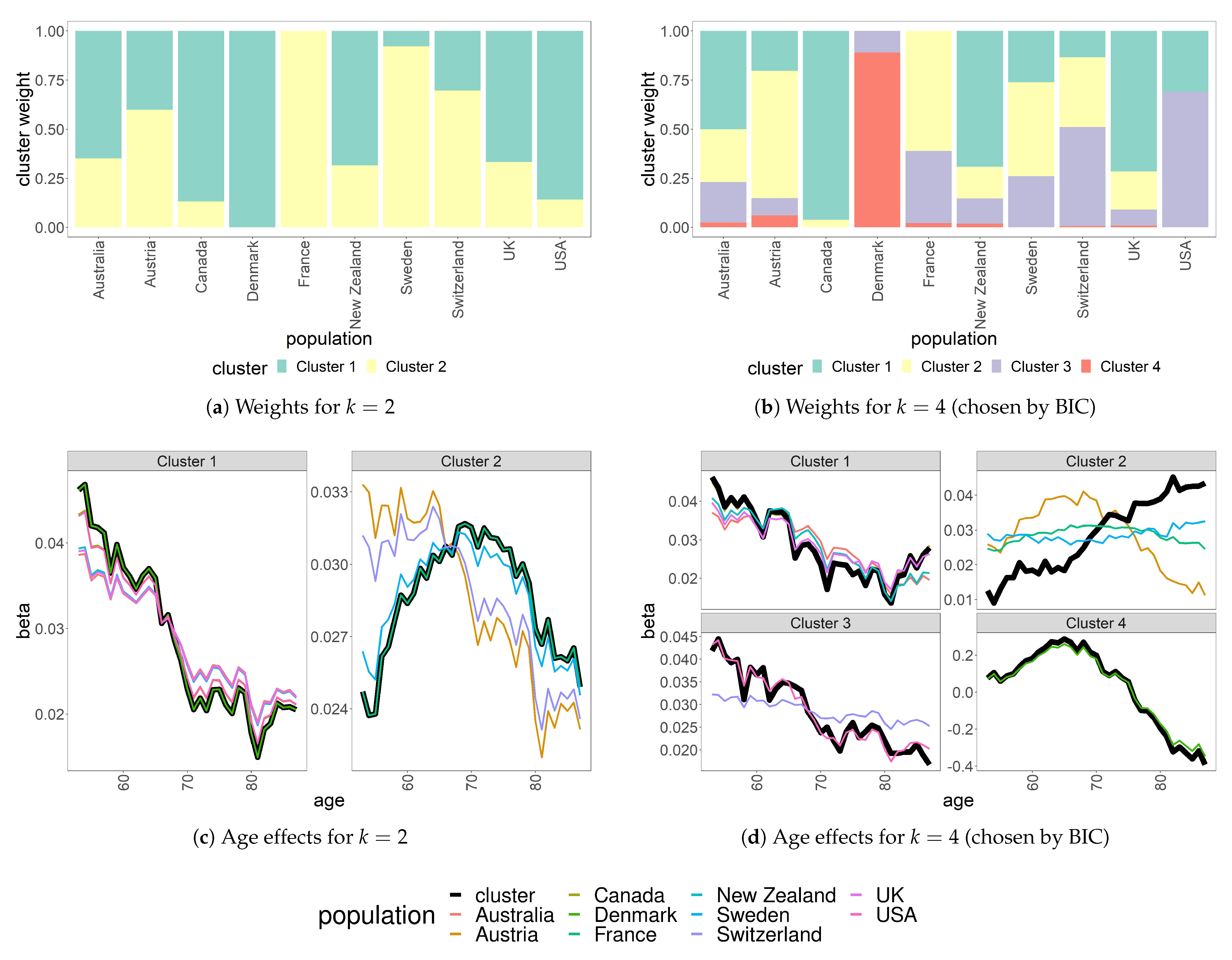
4.2. Clustering Results

Figure 3 displays the population-specific age effects obtained by the ILC model (colored lines) and the cluster-specific age effects obtained by the k-means, ACF-based and likelihood-ratio-based clustering CAE models in comparison to the ordinary CAE model (black lines). Note that for the k-means and likelihood-ratio-based clustering algorithms the ILC age effects are, in fact, inputs. The ACF does not make direct use of the ILC age effects but these are displayed nonetheless for illustration purposes and for an easier graphical overview of the clustering results.

The results of the fuzzy maximum likelihood clustering algorithm are displayed in Figure 4, which shows the cluster membership weights ${\omega }^{i,l}$ in the top row. In the bottom row, we plot the cluster-specific age effects ${\left({\beta }_x^l\right)}_x$ as well as the fitted population-specific age effects ${\left({\sum }_{l=1}^k{\omega }^{i,l}{\beta }_x^l\right)}_x$, where we assign each population $i\in \{1,\dots ,10\}$ to the cluster $l\in \{1,\dots ,k\}$ for which the corresponding weight ${\omega }^{i,l}$ is largest. This clearly illustrates that the fitted age effects are different for all the populations, although for most of them it is also visible that they are a convex combination of a few basic shapes ${\left({\beta }_x^l\right)}_x$, $l=1,\dots ,k$. For $k=2$, we observe that ${\left({\beta }_x^1\right)}_x$ looks similar to the age effect vector in the ordinary CAE model for both age groups, while ${\left({\beta }_x^2\right)}_x$ allows the model to express deviations from the general pattern for some populations.

We provide an overview of the clustering results in

Table 1. Comparison of clustering results obtained by different algorithms for males aged 53 to 87 in 10 countries between 1948 and 1987.

Cluster	k-Means	ACF-Based	Likelihood-Ratio-Based (AL)	Fuzzy ML Clustering ($\mathit{k}=2$)	Fuzzy ML Clustering ($\mathit{k}=4$)
1	AUT	AUS, AUT, CAN, CHE, FRA, SWE, UK, USA	AUS	AUS, CAN, DNK, NZL, UK, USA	AUS, CAN, NZL, UK
2	CHE, FRA, SWE	DNK	AUT, DNK	AUT, CHE, FRA, SWE	AUT, FRA, SWE
3	AUS, CAN, NZL, UK, USA	NZL	CAN	-	CHE, USA
4	DNK	-	FRA, UK	-	DNK
5	-	-	NZL	-	-
6	-	-	SWE, USA	-	-
7	-	-	CHE	-	-

. Most of the clustering algorithms detect that the Danish age effects follow a very distinct pattern, which is due to the stagnation of Danish death rates in the considered time period, and put Denmark into its own cluster. This is in line with the results of Hatzopoulos and Haberman (2013) even though they consider a different data set (ages 0–90, years 1960–2006 and 35 countries). With fuzzy c-means clustering they obtain one West cluster and two East clusters, where all of the populations considered here are in the West cluster but the fuzzy membership weight of Denmark in this cluster is by far the lowest. Two other groups which could be inferred from our clustering results consist of (i) the English-speaking countries Australia, Canada, the UK, the USA and New Zealand and (ii) the remaining European countries France, Sweden, Switzerland and Austria.

In fact, k-means identifies these three groups (Denmark, anglophone countries, remaining European countries) but it assigns Austria to its own cluster. The reason for this gets clearer when we look at the fuzzy maximum likelihood clustering with $k=2$ in Figure 4, where we have imposed NNVM constraints to make the following interpretations sensible (see Section 3.4). Here, the Austrian age effects turn out to be almost a 50:50-mixture of the two fuzzy cluster centers, which can be interpreted as a demonstration of the higher degree of flexibility of the fuzzy maximum likelihood clustering when dealing with observations which are harder to classify. In general, the results are similar to k-means but there are some additional nuances we can recognize, for example, France and Sweden exhibit more similar age effects than France and Switzerland under this model. It is remarkable that Denmark does not get a separate cluster despite its quite special behavior, which might be due to the fact that maximum likelihood estimates are driven by high exposures and the Danish population is rather small. The number of fuzzy clusters which minimizes the BIC is $k=4$, which is the same as for the k-means algorithm. The clustering results are similar as well: Denmark drives its own cluster with only very small shares of other populations (cluster 4), another cluster is driven by Canada with high shares of Australia, New Zealand and the UK (cluster 1). The USA, however, have a higher degree of membership in cluster 3, along with Switzerland, which is separated from France and Sweden, for which the weights are highest in cluster 2 (as well as for Austria).

Before moving on to the results of the ACF and the likelihood ratio clustering, we discuss some observations in the results of k-means and fuzzy clustering which might be counterintuitive at first glance. Looking at Figure 3b, we find that the cluster-specific age effect ${\left({\beta }_x^2\right)}_x$ of the second cluster is very similar to the LC age effect of France. Sweden and Switzerland also belong to this second cluster but their age effects seem to behave quite differently. However, one has to mind the scale of the plots: In fact, the variability of the age effects in cluster 2 is rather small compared to the other clusters. Therefore, while the Swedish and Swiss age effects seem to be very different to the French one on a relative scale, they are nevertheless most similar to it in terms of Euclidean distance compared to the other populations. The observation that the cluster-specific age effect is driven by France results from this age effect being estimated by Poisson maximum likelihood, which is heavily influenced by exposure sizes, and exposures in the French population are substantially larger than in the Swedish and Swiss populations.

Furthermore, in Figure 4 we make the striking observation that the cluster-specific age effect ${\left({\beta }_x^2\right)}_x$ of the second cluster is increasing over ages, whereas the population-specific age effects of all the cluster members (France, Sweden and Austria) are almost constant or even decreasing over ages. To understand this, one has to recall that cluster membership is fuzzy in this case and that all three population-specific age effects are to a significant part influenced by the other cluster-specific age effects as well. Note that ${\left({\beta }_x^1\right)}_x$ and ${\left({\beta }_x^3\right)}_x$ are mostly decreasing with age. Combining these with ${\left({\beta }_x^2\right)}_x$ therefore offsets its increase and yields the almost constant population-specific age effects for France and Sweden. The population-specific age effect of Austria also contains a non-negligible share of ${\left({\beta }_x^4\right)}_x$, the age effect with by far the highest amplitude, which is sufficient to visibly influence the shape of the Austrian age effect in the direction of the age effect of the fourth cluster. In summary, these observations show that population-specific age effects in the fuzzy clustering model are not necessarily similar to any of the cluster-specific age effects. This illustrates the high flexibility of this approach, which allows for individual age effects obtained as linear combinations of a few basic shapes.

The ACF clustering algorithm (with explanation ratio threshold $\eta =0.5$ and improvement threshold $\rho =1$ as chosen by the validation described in Section 3.2) assigns Denmark and New Zealand to separate clusters. All other populations are put into one group together. Likelihood-ratio-based clustering (with average linkage distances and significance level $\sigma ={10}^{-6}$) yields the highest number of groups with separate clusters for Australia, New Zealand, Canada and Switzerland, respectively, and three clusters with two populations each (Austria and Denmark, France and the UK, Sweden and the USA).

We have also performed some experiments on the robustness of the clustering to small changes in the training data. Switching the considered ages from 53–87 to 55–85, we find that the groupings obtained via k-means, ACF clustering and fuzzy clustering for $k=2$ do not change at all while the likelihood-ratio-based clustering and fuzzy maximum likelihood clustering with $k=4$ exhibit slight changes. Adding one more year to the training data (so that the clustering is calibrated on the years 1948 to 1988), we observe that the groupings obtained via k-means and fuzzy clustering do not change at all and ACF clustering merges the cluster consisting of New Zealand into the larger cluster consisting of all other populations except Denmark but remains unchanged apart from that. However, there are again some changes in the results of the likelihood-ratio-based clustering. In conclusion, all of the algorithms with the exception of likelihood-ratio-based clustering exhibit some robustness to small variations of the training data.

We have also run our algorithms for the 16 male populations of the European countries considered by Guibert et al. (2020) (ages 45–90, years 1960–2014). Their hierarchical clustering method, which they apply simultaneously to male and female populations, assigns the male populations to five different clusters. This is exactly the number which is identified as optimal for our fuzzy clustering algorithm albeit with some differences in the composition of the obtained clusters. Populations which are clustered together by both their and our method are (i) West Germany, France, Portugal and Spain, (ii) Finland and Switzerland, (iii) Italy and Luxembourg and (iv) Norway and the Netherlands. If we consider fuzzy clustering with $k=2$, we obtain a cluster consisting of West Germany, Belgium, France, Portugal and Spain—which are the male populations in the first cluster reported by Guibert et al. (2020)—and, additionally, Austria and Switzerland. There are also some similarities between the results of Guibert et al. (2020) and the k-means or likelihood-ratio-based clustering, for example mortality of Danish males being identified as an outlier and assigned its own cluster. However, we also observe several differences in the clustering results. First, this might be due to the fact that our methodology for choosing the number of clusters differs from theirs so that we obtain different cluster sizes at least for the non-fuzzy clustering algorithms (k-means: 8, ACF clustering: 1, likelihood ratio clustering: 12). More importantly, one should recall that, apart from using a different clustering method, Guibert et al. (2020) cluster period effects while we cluster age effects, which may exhibit differing behaviors between populations and, thus, indicate different optimal clustering results.

4.3. Goodness of Fit

For comparing the goodness of fit numerically, we consider the BIC as the main criterion and display it in

Table 2. The BIC and its components (maximal log-likelihood L_max and free number of parameters n_par) for males aged 53 to 87 in 10 countries between 1948 and 1987. The BIC values for the models fitted by Poisson MLE are not directly comparable to those for the models fitted by singular value decomposition (SVD)/common principal components analysis (cPCA).

Model	Lmax	npar	BIC
ACF (SVD)	—	1299	−75,684
CAE (cPCA)	—	774	−78,483
ILC (SVD)	—	1080	−77,550
ILC (MLE)	−86,791	1080	183,893
CAE (MLE)	−91,299	774	189,988
CAE$(k,C)$,
k-means	−87,584	876	183,532
CAE$(k,C)$,
ACF-based	−90,986	842	190,009
CAE$(k,C)$,
LR (av. linkage)	−88,233	978	185,803
CAE Fuzzy,
$k=2$	−87,983	816	183,756
CAE Fuzzy,
$k=4$ (chosen by BIC)	−87,054	894	182,643

. For completeness, we also provide its components, i.e., the maximal value of the log-likelihood function L_max and the free number of parameters n_par (see Section 2.4). Note that the BIC values for the models fitted by Poisson MLE are not directly comparable to those for the models fitted by SVD/cPCA.

We observe that, using maximum likelihood estimation under the assumption of Poisson distributed death counts, the ILC model fits better than the CAE model with respect to the BIC. Interestingly, this is reversed if we calibrate the models via SVD/cPCA, which can also be interpreted as maximum likelihood estimation but under the assumption of a normal distribution of the residuals, see Section 2.4. Among the clustering-based CAE models, k-means and fuzzy maximum likelihood clustering achieve the lowest BIC values, which are in particular considerably lower than those for the ILC model or the CAE model (fitted by Poisson MLE). The BIC penalizes the ILC model for its high number of parameters, while the CAE model has fewer parameters but also a significantly lower log-likelihood value. These findings suggest that the clustering-based CAE models strike a better balance between goodness of fit and parsimony compared to the two extreme cases ILC and ordinary CAE.

We illustrate the goodness of fit graphically by plotting for Denmark and France the actual (red, dashed) and the fitted (black, solid) central death rates at age 67 in Figure 5 (the models were calibrated on all 10 countries, but we depict only two of them for a clearer illustration). We observe that all models show a reasonable fit on visual inspection.

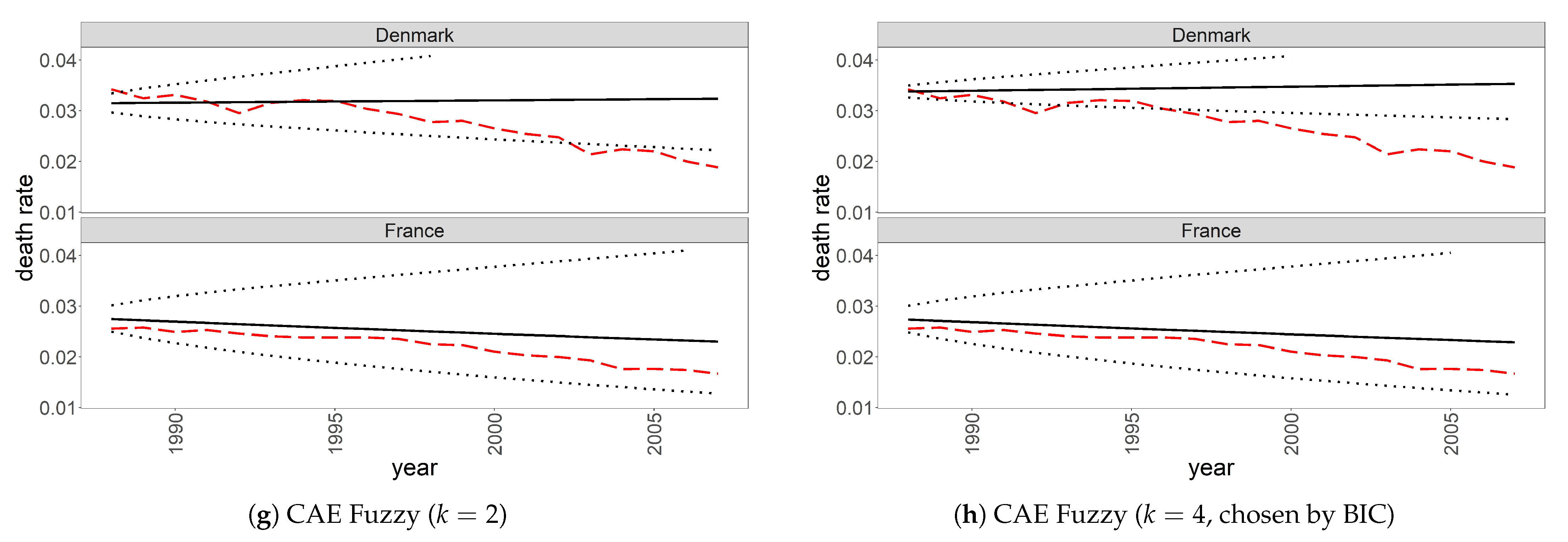
4.4. Forecasting Performance

For evaluating the forecasting performance, we calculate several error measures which are defined in the following and should be minimized in absolute value by the most accurate forecasts:

• $Bias=\frac{1}{N}{\displaystyle \sum _{j=1}^N}\left({\widehat{y}}_j-y_j\right)$,
• mean absolute error, $MAE=\frac{1}{N}{\displaystyle \sum _{j=1}^N}\left|{\widehat{y}}_j-y_j\right|$,
• mean absolute percentage error, $MAPE=\frac{1}{N}{\displaystyle \sum _{j=1}^N}\frac{\left|{\widehat{y}}_j-y_j\right|}{y_j}·100\%$,
• root-mean-square error, $RMSE=\sqrt{\frac{1}{N}{\displaystyle \sum _{j=1}^N}{\left({\widehat{y}}_j-y_j\right)}^2}$,

where we denote the number of forecasts by N, the ground truth by $y_j$ and the forecast by ${\widehat{y}}_j$ and write $j=J(x,t,i)$ with age x, year t, population i and a bijective function J from the set of all tuples $(x,t,i)$ for which a forecast is made to $\{1,\dots ,N\}$.

These out-of-sample error measures are displayed in

Table 3. Out-of-sample error measures for males aged 53 to 87 in 10 countries between 1988 and 2007 (trained on 1948 to 1987). Best values in each column are marked in bold.

Model	Bias	MAE	MAPE	RMSE
ACF (SVD)	5.92‰	6.77‰	20.91%	9.65‰
CAE (cPCA)	5.97‰	6.72‰	19.95%	9.80‰
ILC (SVD)	5.94‰	6.76‰	20.40%	9.99‰
ILC (MLE)	6.01‰	6.75‰	20.38%	10.05‰
CAE (MLE)	6.14‰	6.75‰	19.64%	9.82‰
CAE$(k,C)$,
k-means	6.04‰	6.68‰	20.29%	9.94‰
CAE$(k,C)$,
ACF-based	6.06‰	6.68‰	19.98%	9.65‰
CAE$(k,C)$,
LR (av. linkage)	6.37‰	7.01‰	20.04%	10.58‰
CAE Fuzzy,
$k=2$	5.90‰	6.47‰	19.63%	9.43‰
CAE Fuzzy,
$k=4$ (chosen by BIC)	6.03‰	6.76‰	20.27%	10.16‰

. We generally observe that all models are biased upwards, indicating that mortality has decreased more than they predict based on the given training data. Generally, the ILC and ACF models perform worse than the other models. The CAE fuzzy clustering model with $k=2$ performs best with regard to all error measures. This indicates that the decision to select the value for k by minimizing the BIC, which is a standard approach in the literature, is questionable for this application, as it results in $k=4$ and a significantly worse out-of-sample performance (for lower ages, the optimal number of clusters indicated by the BIC is $k=3$, and this also leads to inferior out-of-sample results compared to $k=2$). Removing the population of Denmark, which as mentioned exhibits a very different fitted age effect pattern compared to the other populations, further enhances the performance of the CAE fuzzy clustering model with $k=2$ (see the corresponding table in the Supplementary Materials).

As a graphical illustration of the projection results, we plot the forecast (black, solid) against the realized (red, dashed) central death rates for age 67 in Figure 6 (the models were calibrated on all 10 countries, but we depict only Denmark and France for a clearer illustration). Additionally, we include $95\%$ prediction intervals (black, dotted). The figures confirm that all models are biased upwards in their out-of-sample projections. Moreover, we find that the uncertainty about these projections differs depending on the model and on the population. The observed death rates for Canada, Denmark and New Zealand decline faster than most models anticipate, even when taking into account forecast uncertainty. In particular, we observe a change in the trend of Danish mortality starting around 1995 which, unsurprisingly, none of the models can foresee.

To check the robustness of our results, we have evaluated the algorithms on three other data sets. Tables with the corresponding out-of-sample error measures can be found in the Supplementary Materials. There, we first present the model-specific error measures for the 21 countries which are considered by Li and Lee (2005) for their illustration of the ACF model. Unsurprisingly, the ACF model shows the best out-of-sample performance for these countries. Among the one-factor models, the fuzzy clustering model with $k=2$ ranks first, in particular clearly outperforming the ordinary CAE model. Moreover, we show a further evaluation for the same 10 populations we have considered throughout this section but for different years, training on 1960 to 1999 and testing on 2000 to 2013. Here, the fuzzy clustering model works better with $k=3$ than with $k=2$ but it dominates the ordinary CAE model with respect to every error measure for both values of k. In addition, it has to be noted that the ILC model fitted via SVD performs surprisingly well for these data. Finally, we have evaluated our clustering-based CAE models and the benchmarks on the 10 populations we have considered in this section with the exception of New Zealand (data only available up to 2013) on even more recent data. We trained the models on the years 1958 to 1997 and evaluated them on the years 1998 to 2017. The results are qualitatively similar to the previous study. Bias and MAPE are minimized by the ILC model fitted via SVD. The fuzzy clustering model with $k=3$ works slightly better than with $k=2$ and clearly better than the ordinary CAE model. The CAE model based on k-means clustering also performs very well, yielding the lowest MAE and RMSE. In summary, we can conclude that no single model stands out as best for all data sets or all error measures. Depending on the data, the clustering-based extensions of the CAE model, in particular the fuzzy clustering model, can be a better alternative than the ordinary CAE model.

As an additional robustness test, a comparison to the out-of-sample performance results of other papers employing clustering methods for mortality forecasting would be interesting. Unfortunately, neither Hatzopoulos and Haberman (2013) nor Guibert et al. (2020) provide such forecasting performance measures, and the results presented by Danesi et al. (2015) refer to a different data set containing mortality data for Italian regions only.

Note that all the results on forecasting performance presented in this section come with the caveat that we have almost exclusively used multivariate, uncorrelated random walks with drift for projection. More sophisticated time series modeling techniques are possible and could greatly enhance forecasting performance. However, our focus lies on an improved modeling of the age effects. The forecasts and performance measures provided serve the purpose of indicating the potential of our proposed model extensions compared to the benchmark models.

5. Conclusions

We have proposed four clustering-based extensions of the common age effect model, which yield age effects specific to groups of populations. In particular, we have investigated a new model inspired by the concept of fuzzy clustering. It has the advantages of giving us an indication which populations are more difficult to cluster and allowing for more modeling flexibility than standard cluster analysis methods like k-means. Comparing our algorithms on the data of 10 populations for ages 53–87, we have found that the majority of algorithms identifies the very distinct pattern of Danish mortality in the considered time period and detects two other groups consisting of the anglophone countries, Australia, Canada, the UK, the USA and New Zealand, on the one hand and the remaining European countries, France, Sweden, Switzerland and Austria, on the other hand.

Our clustering algorithms facilitate a more detailed analysis of historical mortality data of multiple populations and the resulting clustering-based extensions of the CAE model show a better in-sample fit and potentially allow more accurate mortality projections. However, this depends on the data under consideration. The clustering-based models we propose seem to be more recommendable for higher ages for which it might be easier to meaningfully cluster the age effects. Generally, we have found that there is no single model which performs best in every situation, indicating the need to carefully select the model with respect to the specific application and the data under consideration. Finally, we note that, although the absolute differences between the out-of-sample performances of all considered models are mostly rather small, they can nevertheless have a non-negligible financial impact, for example due to the large amounts of money which are typically related to a portfolio of annuities.

There are several ways to extend our model approach, which mostly draw on the existing literature on multi-population mortality modeling.

• Given the availability of data containing features other than age, country and sex such as socioeconomic or health-related characteristics, our clustering-based models could be extended to include such features as well.
• A change point test or similar methods could be applied in order to find the optimal training period instead of selecting it arbitrarily (see Sweeting 2011).
• To make the clustering-based models more parsimonious, populations could not only share the age effect parameters ${\beta }_x$ but also the average mortality level parameters ${\alpha }_x$, which Wen et al. (2020) have found to work well for the standard CAE model. Alternatively, using more parameters to improve the fit, we could also include cohort effects (see Renshaw and Haberman 2006) or more than one age-period interaction term (see Kleinow 2015). For the latter extension, one would need to decide on how exactly the clustering of the age effects is determined.
• We have not devoted much attention to the projection of the ${\kappa }_t$ time series and mostly just used the standard approach, i.e., the random walk with drift. Of course, there are more sophisticated ways to project these time series, for example using general ARIMA models or imposing a non-trivial correlation structure, and thereby ensure coherence or semicoherence (Li et al. 2017) of the projections within the clusters or explicitly model dependencies between the clusters.
• In this regard, it would also be interesting to introduce our clustering algorithms to the locally coherent modeling framework of Guibert et al. (2020). More precisely, all of the clustering algorithms in this paper can potentially be extended to cluster period effects instead of age effects as well. Two aspects which should be addressed in this context are the increased importance of choosing a suitable projection method for the obtained cluster-specific period effects and the necessity of a new identifiability analysis for a fuzzy clustering model on the period effects.
• Our figures clearly show that the estimated age effects lack smoothness, which affects the resulting fitted and projected death rates and, even before that, also might have an undesirable influence on the obtained clustering. It could be beneficial to smooth the ${\beta }_x$ parameters, for example via a penalized log-likelihood approach (see Delwarde et al. 2007). In particular, it would be interesting how this influences the clustering results and how it changes the remaining parameters of the fuzzy maximum likelihood clustering model. Moreover, for the k-means method, other dimension reduction techniques such as PCA (see Debón et al. 2017) could be applied to the age effect vectors as well before performing the clustering.
• With regard to our clustering algorithms, we have found that the BIC as a model selection criterion may lead to suboptimal out-of-sample performance. Other methods for selecting the number of clusters or other hyperparameters of the clustering-based models such as cross validation or the criteria used in Debón et al. (2017) should be investigated, which might lead to a further improvement in the out-of-sample performance of these models as exemplified by the fuzzy maximum likelihood clustering model in Table 3.
• We emphasize once more that the k-means algorithm is only one of many possible clustering methods that can be applied to the framework of Section 3.1. It would be interesting to compare it to other techniques like DBSCAN, spectral clustering or—using a different distance measure—k-medians clustering. In particular, instead of k-means one could also apply the fuzzy c-means algorithm and compare the obtained results to the fuzzy maximum likelihood clustering approach we have proposed (see Hatzopoulos and Haberman 2013).

References

1. Bergeron-Boucher, Marie-Pier, Vladimir Canudas-Romo, Marius D. Pascariu, and Rune Lindahl-Jacobsen. 2018. Modeling and forecasting sex differences in mortality: A sex-ratio approach. Genus 74: 20. [Google Scholar] [CrossRef]
2. Bezdek, James C. 1981. Pattern Recognition with Fuzzy Objective Function Algorithms. Advanced Applications in Pattern Recognition. Boston: Springer. [Google Scholar] [CrossRef]
3. Booth, Heather, John Maindonald, and Len Smith. 2002. Applying Lee-Carter under conditions of variable mortality decline. Population Studies 56: 325–36. [Google Scholar] [CrossRef]
4. Brillinger, David R. 1986. The natural variability of vital rates and associated statistics. Biometrika 42: 693–734. [Google Scholar] [CrossRef]
5. Brouhns, Natacha, Michel Denuit, and Jeroen K. Vermunt. 2002. A Poisson log-bilinear regression approach to the construction of projected lifetables. Insurance: Mathematics and Economics 31: 373–93. [Google Scholar] [CrossRef] [Green Version]
6. Cairns, Andrew J. G. 2014. Modeling and Management of Longevity Risk: Pension Research Council Working Paper, PRC WP2013-19. In Recreating Sustainable Retirement: Resilience, Solvency, and Tail Risk. Edited by Olivia S. Mitchell, Raimond Maurer and P. Brett Hammond. Oxford: Oxford University Press. [Google Scholar] [CrossRef] [Green Version]
7. Cairns, Andrew J. G., David P. Blake, and Kevin Dowd. 2006. Pricing Death: Frameworks for the Valuation and Securitization of Mortality Risk. ASTIN Bulletin 36: 79–120. [Google Scholar] [CrossRef] [Green Version]
8. Cairns, Andrew J. G., David P. Blake, Kevin Dowd, Guy D. Coughlan, David P. Epstein, Alen Ong, and Igor Balevich. 2009. A Quantitative Comparison of Stochastic Mortality Models Using Data From England and Wales and the United States. North American Actuarial Journal 13: 1–35. [Google Scholar] [CrossRef]
9. Cairns, Andrew J. G., David P. Blake, Kevin Dowd, Guy D. Coughlan, and Marwa Khalaf-Allah. 2011. Bayesian Stochastic Mortality Modelling for Two Populations. ASTIN Bulletin 41: 29–59. [Google Scholar]
10. Chen, Hua, Richard MacMinn, and Tao Sun. 2015. Multi-population mortality models: A factor copula approach. Insurance: Mathematics and Economics 63: 135–46. [Google Scholar] [CrossRef]
11. Danesi, Ivan Luciano, Steven Haberman, and Pietro Millossovich. 2015. Forecasting mortality in subpopulations using Lee–Carter type models: A comparison. Insurance: Mathematics and Economics 62: 151–61. [Google Scholar] [CrossRef]
12. Debón, Ana, L. Chaves, Steven Haberman, and F. Villa. 2017. Characterization of between-group inequality of longevity in European Union countries. Insurance: Mathematics and Economics 75: 151–65. [Google Scholar] [CrossRef] [Green Version]
13. Delwarde, Antoine, Michel Denuit, and Paul H. C. Eilers. 2007. Smoothing the Lee–Carter and Poisson log-bilinear models for mortality forecasting. Statistical Modelling: An International Journal 7: 29–48. [Google Scholar] [CrossRef]
14. Delwarde, Antoine, Michel Denuit, Montserrat Guillén, and A. Vidiella. 2006. Application of the Poisson log-bilinear projection model to the G5 mortality experience. Belgian Actuarial Bulletin 6: 54–68. [Google Scholar]
15. Enchev, Vasil, Torsten Kleinow, and Andrew J. G. Cairns. 2017. Multi-population mortality models: Fitting, forecasting and comparisons. Scandinavian Actuarial Journal 2017: 319–42. [Google Scholar] [CrossRef] [Green Version]
16. Giordano, Giuseppe, Steven Haberman, and Maria Russolillo. 2019. Coherent modeling of mortality patterns for age-specific subgroups. Decisions in Economics and Finance 42: 189–204. [Google Scholar] [CrossRef] [Green Version]
17. Guibert, Quentin, Stéphane Loisel, Olivier Lopez, and Pierrick Piette. 2020. Bridging the Li-Carter’s Gap: A Locally Coherent Mortality Forecast Approach. Preprint. Available online: https://hal.archives-ouvertes.fr/hal-02472777 (accessed on 19 February 2021).
18. Hastie, Trevor, Robert Tibshirani, and Jerome Friedman. 2017. The Elements of Statistical Learning: Data Mining, Inference, and Prediction, 2nd ed. Berlin: Springer. [Google Scholar]
19. Hatzopoulos, Peter, and Steven Haberman. 2013. Common mortality modeling and coherent forecasts. An empirical analysis of worldwide mortality data. Insurance: Mathematics and Economics 52: 320–37. [Google Scholar] [CrossRef]
20. Human Mortality Database. 2019. University of California, Berkeley (USA), and Max Planck Institute for Demographic Research, Rostock (Germany). Available online: https://www.mortality.org (accessed on 2 July 2019).
21. Hyndman, Rob J., Heather Booth, and Farah Yasmeen. 2013. Coherent mortality forecasting: The product-ratio method with functional time series models. Demography 50: 261–83. [Google Scholar] [CrossRef] [Green Version]
22. Kleinow, Torsten. 2015. A common age effect model for the mortality of multiple populations. Insurance: Mathematics and Economics 63: 147–52. [Google Scholar] [CrossRef] [Green Version]
23. Kleinow, Torsten, and Andrew J. G. Cairns. 2013. Mortality and smoking prevalence: An empirical investigation in ten developed countries. British Actuarial Journal 18: 452–66. [Google Scholar] [CrossRef] [Green Version]
24. Lee, Ronald D. 2000. The Lee-Carter Method for Forecasting Mortality, with Various Extensions and Applications. North American Actuarial Journal 4: 80–91. [Google Scholar] [CrossRef]
25. Lee, Ronald D., and Lawrence R. Carter. 1992. Modeling and Forecasting U.S. Mortality. Journal of the American Statistical Association 87: 659–71. [Google Scholar] [CrossRef]
26. Léger, Ainhoa-Elena, and Stefano Mazzuco. 2020. What Can We Learn from Functional Clustering of Mortality Data? An Application to HMD Data. Preprint. Available online: http://arxiv.org/pdf/2003.05780v1 (accessed on 19 February 2021).
27. Li, Johnny S.-H., Wai-Sum Chan, and Rui Zhou. 2017. Semicoherent Multipopulation Mortality Modeling: The Impact on Longevity Risk Securitization. Journal of Risk and Insurance 84: 1025–65. [Google Scholar] [CrossRef]
28. Li, Johnny S.-H., Rui Zhou, and Mary R. Hardy. 2015. A step-by-step guide to building two-population stochastic mortality models. Insurance: Mathematics and Economics 63: 121–34. [Google Scholar] [CrossRef]
29. Li, Nan, and Ronald D. Lee. 2005. Coherent Mortality Forecasts for a Group of Populations: An Extension of the Lee-Carter Method. Demography 42: 575–94. [Google Scholar] [CrossRef] [Green Version]
30. Meslé, France, and Jacques Vallin. 2002. Mortalité en Europe: la divergence Est-Ouest. Population 57: 171. [Google Scholar] [CrossRef]
31. Nielsen, Bent, and Jens P. Nielsen. 2010. Identification and Forecasting in the Lee-Carter Model. Working Paper. Available online: https://ssrn.com/abstract=1722538 (accessed on 19 February 2021).
32. Oppers, S. Erik, Ken Chikada, Frank Eich, Patrick Imam, John Kiff, Michael Kisser, Mauricio Soto, and Tao Sun. 2012. The Financial Impact of Longevity Risk. In Global Financial Stability Report—The Quest for Lasting Stability. Washington, DC: International Monetary Fund, Chapter 4. [Google Scholar]
33. Pitacco, Ermanno, Michel Denuit, Steven Haberman, and Annamaria Olivieri. 2008. Modelling Longevity Dynamics for Pensions and Annuity Business. Oxford: Oxford University Press. [Google Scholar]
34. R Core Team. 2019. R: A Language and Environment for Statistical Computing. Vienna: R Core Team. [Google Scholar]
35. Renshaw, Arthur E., and Steven Haberman. 2006. A cohort-based extension to the Lee–Carter model for mortality reduction factors. Insurance: Mathematics and Economics 38: 556–70. [Google Scholar] [CrossRef]
36. Sweeting, Paul J. 2011. A Trend-Change Extension of the Cairns-Blake-Dowd Model. Annals of Actuarial Science 5: 143–62. [Google Scholar] [CrossRef]
37. Villegas, Andrés M., Steven Haberman, Vladimir K. Kaishev, and Pietro Millossovich. 2017. A comparative study of two-populations models for the assessment of basis risk in longevity hedges. ASTIN Bulletin 47: 631–79. [Google Scholar] [CrossRef] [Green Version]
38. Wen, Jie, Andrew J. G. Cairns, and Torsten Kleinow. 2020. Fitting Multi-Population Mortality Models to Socio-Economic Groups. Annals of Actuarial Science (to appear). [Google Scholar] [CrossRef]
39. Wen, Jie, Torsten Kleinow, and Andrew J. G. Cairns. 2020. Trends in Canadian Mortality by Pension Level: Evidence from the CPP and QPP. North American Actuarial Journal 41: 1–29. [Google Scholar] [CrossRef]
40. Wickham, Hadley. 2016. Ggplot2: Elegant Graphics for Data Analysis/Hadley Wickham; with Contributions by Carson Sievert, Use R! 2nd ed. Switzerland: Springer. [Google Scholar]
41. Zhou, Rui, Johnny S.-H. Li, and Ken S. Tan. 2013. Pricing Standardized Mortality Securitizations: A Two-Population Model With Transitory Jump Effects. Journal of Risk and Insurance 80: 733–74. [Google Scholar] [CrossRef]
42. Zugic, Richard, Gavin Jones, Costas Yiasoumi, Kerry McMullan, Andreas Tacke, Michael Held, and Benoit Moreau. 2010. Longevity. Position Paper, CRO Forum. Available online: https://www.thecroforum.org/wp-content/uploads/2010/11/Longevity-Risk.pdf (accessed on 19 February 2021).
Figure 1. Dendrograms for between-cluster distances (left: single linkage, mid: complete linkage, right: average linkage) based on mortality data for males aged 53 to 87 in 10 countries between 1948 and 1987 (note the differing scales).
Risks 09 00045 g001
Figure 2. Death rates for males aged 53, 60, 67, 74, 81 and 87 in Denmark, France and the USA between 1948 and 2007 (note the differing scales).
Risks 09 00045 g002
Figure 3. Age effects by cluster for males aged 53 to 87 in 10 countries between 1948 and 1987 obtained by the common age effect (CAE) model and three of its clustering-based extensions. The age effects of the clusters are displayed in black and the individual Lee–Carter (ILC) age effects of the populations are in different colors.
Risks 09 00045 g003
Figure 4. Weights ω i , l (top) and cluster-specific age effects β x l x as well as fitted population-specific age effects l = 1 k ω i , l β x l x (bottom) of the fuzzy maximum likelihood clustering for males aged 53 to 87 in 10 countries between 1948 and 1987.
Risks 09 00045 g004
Figure 5. Actual (red, dashed) and fitted (black, solid) central death rates for males aged 67 in Denmark and France (models calibrated on 10 countries) between 1948 and 1987.
Risks 09 00045 g005aRisks 09 00045 g005b
Figure 6. Actual (red, dashed) and forecast (black, solid) central death rates and 95 % prediction intervals (black, dotted) for males aged 67 in Denmark and France (models calibrated on 10 countries) between 1988 and 2007.
Risks 09 00045 g006aRisks 09 00045 g006b