Mortality Forecasting with an Age-Coherent Sparse VAR Model

Abstract

This paper proposes an age-coherent sparse Vector Autoregression mortality model, which combines the appealing features of existing VAR-based mortality models, to forecast future mortality rates. In particular, the proposed model utilizes a data-driven method to determine the autoregressive coefficient matrix, and then employs a rotation algorithm in the projection phase to generate age-coherent mortality forecasts. In the estimation phase, the age-specific mortality improvement rates are fitted to a VAR model with dimension reduction algorithms such as the elastic net. In the projection phase, the projected mortality improvement rates are assumed to follow a short-term fluctuation component and a long-term force of decay, and will eventually converge to an age-invariant mean in expectation. The age-invariance of the long-term mean guarantees age-coherent mortality projections. The proposed model is generalized to multi-population context in a computationally efficient manner. Using single-age, uni-sex mortality data of the UK and France, we show that the proposed model is able to generate more reasonable long-term projections, as well as more accurate short-term out-of-sample forecasts than popular existing mortality models under various settings. Therefore, the proposed model is expected to be an appealing alternative to existing mortality models in insurance and demographic analyses.

1. Introduction

The ongoing improvement of human life expectancy around the world has made longevity risk, the risk that people live longer than expected, an increasingly important risk for many demographic, economic, and insurance practices. This has urged the academia to better understand the driving factors of mortality improvements, and design effective statistical tools to provide accurate and credible mortality projections.

The past few decades have witnessed rapid developments of mortality forecasting research. Among existing methods, one popular class of model is the so called factor-based models. These models use factor representations to summarize mortality patterns of high dimensional data sets by one or few factors. Mortality projections are then obtained by extrapolating the estimated factors. To date, the most widely used factor-based models include the Lee–Carter model (Lee and Carter 1992) and the Cairns–Blake–Dowd (Cairns et al. 2006) model. Many extensions of these two models have been proposed in the literature (see, among many others, Booth et al. 2006; Li et al. 2015; Li and Li 2017; Li et al. 2019; Renshaw and Haberman 2006). While the Lee–Carter and the CBD models have been demonstrated to be effective in mortality forecasting, they are not able to explicitly model mortality correlations between different populations, as only one population can be fitted at a time. To address the modeling of joint mortality dynamics, Li and Lee (Li and Lee 2005) extend the Lee–Carter model to a multi-population context, in which mortality rates of all populations are assumed to follow a common systematic trend. In particular, mortality projections generated by the Li–Lee model is population-coherent, i.e., the projected mortality rates of different populations at the same age will not diverge in the long run. Since the Li–Lee model, coherent multi-population mortality modelling has drawn increasing attention in the literature (see, for example, Dowd et al. 2011; Hyndman et al. 2013).

While the factor-based models are effective in forecasting mortality rates, especially when the cross-section dimension (age) of the underlying data is large, there are still limitations associated with these models. In particular, these models typically have fixed age effects (i.e., loadings to the factors), and are thus likely to generate diverging mortality forecast at different ages (Li et al. 2013). In other words, while the Li–Lee model is population-coherent, it is not age-coherent. Moreover, as argued by Hunt and Blake (2018), many factors representations suffer from identifiability issue when cohort effects are included. To address this issue, vector-autoregressive (VAR) models have been proposed to study and forecast mortality (Guibert et al. 2019; Li and Lu 2017; Li and Shi 2020). Compared to the factor-based models, VAR models have more flexible parametric structures, and thus could better capture the potentially complicated mortality patterns underlying the data. However, the estimation of VAR mortality models is often challenging because of the high dimension of mortality data sets. In particular, it is often the case that the cross-section dimension is larger than the time dimension, and thus the estimation of unconstrained VAR mortality models is impossible. Consequently, dimension reduction techniques of the coefficient matrix are required. For example, Li and Lu (2017) simplify the coefficient matrix by allowing for only one nonzero period effect and two cohort effects, and the resulting model is referred to as the spatial-temporal (STAR) model. Under this assumption, they derive age-coherent and population-coherent mortality projections, i.e., the projected mortality rates of any two ages in any two populations will not diverge in the long-run. The simple STAR model in Li and Lu (2017) is later extended by many studies, including Chang and Shi (2020a), Chang and Shi (2020b), and Shi (2020). On the other hand, Guibert et al. (2019) adopted a pure data-driven approach for mortality modeling using the sparse VAR model with an elastic-net (ENET) penalty, which we refer to as the SVAR model. Compared to the STAR model, the SVAR model is more objective, as more period and cohort effects can be included in the regression, depending on their explanatory power of the mortality rates modelled. However, the SVAR model focuses on the mortality improvement rates, instead of the original mortality rates, and hence the co-integration relations cannot be explicitly addressed. Consequently, mortality projections generated by the SVAR model are not age-coherent nor population-coherent.

In this paper, we propose a coherent sparse vector-autoregressive (CSVAR) model which combines the appealing features of both the STAR model and the SVAR model. In particular, the proposed CSVAR model utilizes the data-driven algorithms, to determine the period, age, and cohort effects that should be included in each regression, and meanwhile propose a rotation algorithm of the long-term mean of each age-specific mortality series to ensure age-coherent projections. The model is estimated in two steps. First, age-specific mortality improvement rates are fitted to a VAR model with data-driven dimension reduction techniques, such as LASSO or elastic-net. Then, in the projection phase, the intercepts (expectations) of mortality improvement rates are assumed to follow a time-series dynamics and converge to a long-term limit. By letting the long-term limit be age-invariant, the difference between projected mortality rates of any two ages will be bounded in the long-term. Hence, projected mortality rates generated by the proposed CSVAR model are age-coherent. The idea of converging the long-term mean of mortality improvement rates has the same spirit as the mortality rotation method discussed in Li et al. (2013) and Li et al. (2018). Furthermore, the proposed CSVAR model can be extended to modeling the joint mortality dynamics of multiple populations in a computationally efficient manner. In the latter case, the long-term limit of mortality improvement rates will be assumed invariant to both age and population, so the projected mortality rates will be both age- and population-coherent.

In the empirical analysis, the proposed CSVAR model is illustrated using the single-age, uni-sex mortality data of the UK and France in both the single-population and multi-population context. We find that, due to the age-coherent feature, the CSVAR model generates smoother long-term projection of age-specific mortality rates. In particular, the projected mortality improvements are more similar across ages—they are more pronounced for the old ages and less substantial for the very young ages compared to those produced by the Lee–Carter model and the SVAR model. As a result, the proposed CSVAR generates higher point forecasts of life expectancy at birth than the Lee–Carter model and the STAR model at all forecast horizons. Moreover, in the out-of-sample forecast analysis, the proposed CSVAR model is able to produce more accurate out-of-sample forecasting results than the Lee–Carter model (and the Li–Lee model in the multi-population case) and the SVAR model with different choices of sample size and age groups. Furthermore, the proposed CSVAR model produces projected life expectancy closer to the realized values over the out-of-sample forecast period in both populations than the Lee–Carter model and the STAR model. Therefore, it seems that the proposed CSVAR model is able to generate both the long-term forecasts and the short-term out-of-sample forecasts, and could therefore be a appealing alternative to the existing models in life insurance and demographic analysis.

The remainder of the paper is organized as follows. Section 2 reviews the Lee–Carter model and the Li–Lee model. Section 3 reviews the existing VAR-based mortality models, especially the SVAR model, and introduces the age-coherent CSVAR model. Section 4 discusses the empirical analysis. Section 5 concludes the paper.

2. The Factor-Based Model

Suppose we have mortality data of N ages, each age with T years of observations. The Lee–Carter (LC) model (Lee and Carter 1992) summarizes the systematic mortality trends of the N ages by a common factor. Formally, the log central mortality rate at age x in year t, $y_{x,t}$, follows the specification given by:

$$y_{x,t}=a_x+b_x{k}_t+{\epsilon }_{x,t},$$

(1)

where $a_x$ is the mortality level, i.e., the average mortality rate over time at age x, $k_t$ is the period effect, i.e., the systematic mortality trend common to all ages, $b_x$ is the age effect at x, i.e., the sensitivity of $y_{x,t}$ to $k_t$, and ${\epsilon }_{x,t}$ is the normal residual term with mean 0 and variance ${\sigma }_{{\epsilon }_x}^2$. As noted by Lee and Carter (1992), Equation (1) is not identifiable without normalization constraints. For example, one could multiply $b_x$ with a constant c and divide $k_t$ by the same constant, and reach the same fitting results. In Lee and Carter (1992), the following normalization constraints are imposed:

$$\sum _t{k}_t=0, \text{and}\sum _x{b}_x=1.$$

(2)

Given the first constraint, $a_x$ is set to the mean of $y_{x,t}$ over the sample considered. The Lee–Carter model is then estimated by singular value decomposition (SVD) instead of the usual ordinary least square approach in the original paper1. Given the estimated $a_x$ and $b_x$, $k_t$ is adjusted to match the fitted total number of deaths to the observed values in each year t. This adjustment rebalances the contribution of age-specific mortality by assigning greater weights to ages with a larger number of death.

While $a_x$ and $b_x$ are assumed to be constant, the period effect is often modelled by a time-series process. In particular, Lee and Carter (1992) assumes a random walk with drift specification, which is adopted by many later studies:

$$k_t=k_{t-1}+d+e_t,$$

(3)

where the drift term d measures the average annual change in $k_t$, and $e_t\stackrel{i.i.d.}{\sim }N(0,{\sigma }_e^2)$. Based on the time-series specification in Equation (3), future mortality rates can be projected by extrapolating the period effect $k_t$. Specifically, the expected h-step-ahead mean forecasts of the period effect and the log central death rate are given by:

$$\begin{array}{cc}\hfill {\hat{k}}_{T+h}& =k_T+hd,\hfill \\ \hfill {\hat{y}}_{x,T+h}& =a_x+b_x{\hat{k}}_{T+h},\hfill \end{array}$$

(4)

where T is last year of the sample.

The Lee–Carter model is a single-population model, i.e., it focuses on the mortality of one population at a time. This constraint is later relaxed by the Li–Lee model (Li and Lee 2005), which incorporates mortality dynamics of multiple populations simultaneously. The joint modeling of mortality dynamics of multiple populations are important not only in demographic analysis (Li et al. 2019), but also for various insurance practices, including the risk management of insurance policies for small portfolios and the pricing of the innovative index-based longevity-linked securities and retirement products (Chen et al. 2020; Li 2018; Li et al. 2017; Li and Lu 2018, 2019). In the Li–Lee model, the log central death rates are represented by a common factor and a population-specific factor. Suppose there are I populations in total, the log central death rate for the i-th population at age x and year t, $y_{x,t,i}$, follows the specification given by:

$$y_{x,t,i}=a_{x,i}+B_x{K}_t+b_{x,i}{k}_{t,i}+{\epsilon }_{x,t,i},i=1,\dots ,I,$$

(5)

where $a_{x,i}$ is the average mortality level at age x in the ith population, $B_x$ and $K_t$ represent the common age effect and period effect, $k_{t,i}$ is the population-specific period effect with respect to the ith population, and $b_{x,i}$ is the corresponding population-specific age effect. Finally, ${\epsilon }_{x,t,i}$ is the normal population-specific error term with mean 0 and variance ${\sigma }_{{\epsilon }_{x,i}}^2$. Similarly, a set of normalization constraints are imposed to ensure identifiability:

$$\begin{array}{cc}\hfill \sum _t{K}_t=0,& \text{and}\sum _x{B}_x=1,\hfill \\ \hfill \sum _t{k}_{t,i}=0,& \text{and}\sum _x{b}_{x,i}=1.\hfill \end{array}$$

(6)

Similar to the Lee–Carter model, the common period effect $K_t$ can be modelled as a random walk with drift process. On the other hand, the population-specific period effects $k_{t,i}$, $i=1,\dots ,I$ are fitted by stationary autoregressive processes to ensure coherent forecasts in the long term. Specifically, the time-series specifications of the period effects are given by:

$$\begin{array}{cc}\hfill K_t& =K_{t-1}+d+e_t,\hfill \\ \hfill k_{t,i}& =a_{0,i}+a_{1,i}{k}_{t-1,i}+e_{t,i},\hfill \end{array}$$

(7)

where $a_{0,i}$ and $|a_{1,i}|<1$ are the autoregressive parameters and $e_{t,i}$ is the Gaussian error term with mean 0 and variance ${\sigma }_{e_i}^2$. Stationarity of the $k_{i,t}$ processes guarantees that deviations of the projected mortality of each population from each other will not grow infinitely in the long run. Formally, the projected mortality rates are coherent for different populations in the long-run if ${\hat{y}}_{x,T+h,i}-{\hat{y}}_{x,T+h,j}=O_p\left(1\right)$ for $i\ne j$. We see that this condition is indeed satisfied if all $k_{i,t}$s are stationary, as in this case the long-term mortality trends of all ages and populations are driven by the single common period effect $K_t$, and $k_{i,t}$s only represent the short-term fluctuations around the common mortality trend. Therefore, the Li–Lee model is indeed able to generate coherent mortality projections across populations. However, as noted by recent studies (for example, Li and Lu 2017), the coherent property only holds for projected mortality rates of the same age. Specifically, for an arbitrary different age $z\ne x$, the Li–Lee model will not lead to ${\hat{y}}_{x,T+h,i}-{\hat{y}}_{z,T+h,j}=O_p\left(1\right)$ for any i and j. Therefore, the mortality projections generated by the Li–Lee model is not age-coherent.

3. The Vector-Autogression-Based Models

As an alternative to factor-based models, VAR-based mortality models have been a rapidly emerging class of mortality models in recent literature. Compared to the factor-based models, the VAR-based are more flexible and thus able to capture more complex time, age, and cohort mortality dependence (Guibert et al. 2019; Li and Lu 2017). However, the application of VAR-based models in mortality forecasting leads to new challenge. In particular, unconstrained VAR models typically have a larger number of parameters to be estimated, while observations in mortality data are often limited. For example, suppose we have N age groups and only one population is considered. Even in the simplest VAR(1) case, if the first order lag of all the N ages are included, then the total number of parameters will be $p=N(N+1)$ (including N intercepts), while the total number of observations is $NT$. In mortality analysis, we typically have only a few decades of annual data, while the number of ages could be above 100. Therefore, there are typically more unknown parameters than observations in the standard VAR framework without any parameter constraints.

3.1. The Sparse VAR Model

A recent effort to address the curse of dimenisonality issue in the VAR mortality models is made by Guibert et al. (2019), who employ a sparse VAR (SVAR) model on mortality improvements. First, they model the dynamics of the mortality improvement rates, $\Delta y_{x,t}=y_{x,t}-y_{x,t-1}$, rather than the mortality rates themselves. Under the assumption that ${\left(y_{x,t}\right)}_t$ is an $I\left(1\right)$ process for all ages, the dependent variables ${(\Delta y_{x,t})}_t$ are $I\left(0\right)$ and therefore stationary. As a result, standard VAR models can be used, without the need to consider co-integration relations within mortality data. Second, using an elastic-net (ENET) penalty estimation, the SVAR model adopts a pure data-driven method to select the non-zero coefficients in the estimation process. In this way the coefficient matrix will be sparse, i.e., the majority of autoregressive coefficients will be set to zero. Formally, when only the first order lage is considered, the mortality improvement model is given by:

$$\Delta {\mathbf{Y}}_{\mathbf{t}}=\mathbf{M}+\mathbf{B}\Delta {\mathbf{Y}}_{\mathbf{t}-1}+{\mathit{\epsilon }}_t,$$

(8)

where $\Delta {\mathbf{Y}}_{\mathbf{t}}$= ${(\Delta y_{1,t},\Delta y_{2,t},\dots ,\Delta y_{N,t})}^{\prime }$ is the $N\times 1$ vector of mortality improvement rates. ${\mathit{\epsilon }}_t$ is assumed to follow a multi-Gaussian distribution with mean 0. $\mathbf{M}$ is an $N\times 1$ vector estimated by the sample averages of $\Delta {\mathbf{Y}}_{\mathbf{t}}$. $\mathbf{B}$ is the coefficient matrix, and the sparsity (frequency and location of zeros) of $\mathbf{B}$ is determined by the LASSO (L1) penalty during the estimation process without any constraints. More specifically, the objective function to be minimized is given by:

$$\begin{array}{c}\hfill (\hat{\mathbf{M}},\hat{\mathbf{B}})=arg\underset{\mathbf{M}\in R^N,\mathbf{B}\in R^{N\times N}}{min}\frac{1}{2}\sum _{t=1}^T\parallel {\mathbf{y}}_t-\mathbf{M}-\mathbf{B}{\mathbf{y}}_{t-1}{\parallel }_2^2+\lambda \sum _{i,j}^N\left|{\beta }_{ij}\right|,\end{array}$$

(9)

where ${\beta }_{i,j}$ is the ith row jth column element of $\mathbf{B}$, and $\lambda$ is the L1 penalty parameter. A larger value of $\lambda$ will shrink more ${\beta }_{i,j}$ to be exactly 0. The selection of $\lambda$ is performed via the cross validation with ten-fold, and the estimates of parameters are then obtained accordingly. Details can be found in Friedman et al. (2010). After estimating Model (8), the forecasting is performed as follows:

$$\begin{array}{cc}\hfill \Delta {\hat{\mathbf{Y}}}_{T+h}& =\hat{\mathbf{M}}+\hat{\mathbf{B}}\Delta {\hat{\mathbf{Y}}}_{T+h-1},\hfill \end{array}$$

(10)

with $h>1$. As a result, it holds that ${\hat{\mathbf{Y}}}_{T+h}={\mathbf{Y}}_{\mathbf{T}}+$${\sum }_{l=1}^h$$\Delta {\hat{\mathbf{Y}}}_{T+l}$.

In a I-population case, we may let $\Delta {\mathbf{Y}}_{\mathbf{t}}$ be an $NI\times 1$ vector given by ${(\Delta y_{1,t,1},\dots ,\Delta y_{N,t,I})}^{\prime }$, where $\Delta y_{x,t,i}$ is the mortality improvement rate of the i-th population at age x and year t. Other variables and parameters of Equation (8) can be redefined accordingly in a straightforward manner. In all cases, the sparsity of $\mathbf{B}$ depends on the tuning parameter $\lambda$ in the estimation process, which is derived via the usual cross-validation procedure. Given Equations (8)–(10), we see that ${\hat{y}}_{x,T+h}-{\hat{y}}_{x+k,T+h}=O_p\left(1\right)+O_p\left(h\right)({\hat{m}}_x-{\hat{m}}_{x+k})$ for two arbitrary ages x and $x+k$ in the SVAR model, because $\Delta y_{x,t}$ is stationary for any x. As a result, without any constraints on ${\hat{m}}_x$ and ${\hat{m}}_{x+k}$, the projected mortality rates of any two ages will be diverging in the long-run, and thus the projection generated by the SVAR model is not age-coherent either.

3.2. The Coherent Sparse VAR Model

In this paper we propose a age-coherent extension of the SVAR model introduced in Section 3.1 by generalizing the intercepts in the projection, i.e., $\hat{\mathbf{M}}$ in Equation (10), will be extended to a series of stationary time-dependent processes. Specifically, the x-th element of $\hat{\mathbf{M}}$, ${\hat{m}}_x$, will be generalized to a process ${\left({\hat{m}}_{x,h}\right)}_h$ which varies over the projection horizon and converges in expectation to a constant universal to all ages, and therefore the projected mortality rates of all ages will be non-diverging in the long-run. To this end, many stationary processes can be chosen. In this paper, we illustrate the proposed method using the hyperbolic decay process. In time-series analysis, the hyperbolic decay is related to the concept of long memory (Feng and Shi 2017; Gao et al. 2020; Ho and Shi 2020), representing the type of decay with speed slower than that of the short memory ones, such as the geometric or exponential decay processes (Hosking 1981). An application of the hyperbolic decay in the mortality modelling and forecasting can be found in Feng et al. (2020). Formally, under the assumption of hyperbolic decay, the intercept used in the $h-$step ahead forecast, ${\hat{m}}_{x,h}$, is given by:

$${\hat{m}}_{x,h}={\delta }_h\left(d_x\right)({\hat{m}}_x-{\hat{m}}^{*})+{\hat{m}}^{*},$$

(11)

where ${\hat{m}}_x$ is defined in the same way as in Equation (8), ${\hat{m}}^{*}$ is long-term mean of ${\hat{m}}_x$ for all xs, and the hyperbolic parameter ${\delta }_h\left(d_x\right)$ is defined as:

$${\delta }_h\left(d_x\right)=\frac{h-1+d_x}{k}{\delta }_{h-1}\left(d_x\right)\text{and}{\delta }_0\left(d_x\right)=1.$$

(12)

When the hyperbolic parameter $d_x$ falls between 0 and 1, it holds that ${\delta }_h\left(d_x\right)\to 0$ when $h\to \infty$, and ${\hat{m}}_{x,h}$ will eventually converge (decay) to ${\hat{m}}^{*}$. Furthermore, the speed of decay is slower (resp. faster) for larger (resp. smaller) values of $d_x$. The extension from a constant $\hat{\mathbf{M}}$ to the hyperbolic decay processes of intercepts then leads to age-coherent projection of mortality rates. More specifically, for any two ages x and $x+k$, the distance between the projected mortality rates h steps ahead is given by:

$$\begin{array}{cc}\hfill & {\hat{y}}_{x,T+h}-{\hat{y}}_{x+k,T+h}\hfill \\ \hfill =& O_p\left(1\right)+O_p\left(h\right)({\hat{m}}_x-{\hat{m}}_{x+k})\hfill \\ \hfill =& O_p\left(1\right)+O_p\left(h\right)({\hat{m}}^{*}-{\hat{m}}^{*})\hfill \\ \hfill =& O_p\left(1\right),\hfill \end{array}$$

(13)

which will stay bounded in the long run. In this paper, we let ${\hat{m}}^{*}$ be the sample mean of all ${\hat{m}}_x$, and refer to the model with the time-varying intercepts given in Equation (11) as the coherent SVAR (CSVAR) model.

Despite the aforementioned desirable feature of age-coherent forecasts, the determination of $d_x$ is a non-trivial issue in the CSVAR model. There are two major challenges. First, without parameter restrictions, the introduction of $d_x$ could increase the number of parameters by N ($d_1$, …, $d_N$). To address this issue, an appropriate dimensionality reduction technique is required. In particular, as argued in Li and Lu (2017), mortality changes of neighboring ages are typically rather smooth. Therefore, it is reasonable to assume that $d_x$ is a smooth function of x for each age to cope with the empirical patterns. Furthermore, it is argued in existing studies that mortality declined will be lower at older ages (see, for example, Li et al. 2013). This suggests that appropriate functional forms should be imposed such that $d_x$ is smaller for larger xs, and thus the corresponding ${\hat{m}}_{x,h}$s will converge to ${\hat{m}}^{*}$ more slowly. Second, as the parameters $d_x$s only play a role in the projection phase, there is no data to identify the optimal parametric structure of $d_x$ (over x). In particular, the historical data were already used to estimate $\hat{\mathbf{M}}$. Thus, in order to identify the parametric structure of $d_x$, estimation procedures such as cross-validation should be employed.

To deal with the first challenge, in this paper we use the inverse Epanechnikov kernel evaluated at the last observation to characterize the parametric structure of $d_x$. Inverse Epanechnikov kernel is a parsimonious approach to construct smooth functions. More specifically, let $\tau$ be the scaled index $x/N$ with $x\in (1,\dots ,N)$, the (adjusted) inverse Epanechnikov kernel evaluated at N is determined by $1-K_b(\tau -1)=1-K\left(\frac{\tau -1}{b}\right)$ with $K(\tau -1)=0.75[1-{(\tau -1)}^2]$. The parameter b, ranging from 0 to 1, is the bandwidth of the inverse Epanechnikov kernel. For example, consider ages 0–100, the inverse Epanechnikov kernels evaluated at age 100 is displayed in Figure 1 for $b=$ 0.1, 0.25, 0.5, 0.75 and 1. We see that the estimated kernel $1-K_b(\tau -1)$ is constant for all ages up to a “cut-off” age, and then become decreasing afterwards. Specifically, the cut-off age is determined by the bandwidth parameter b. For example, if $b=0.1$, then the cut-off is the 90% percentile of all ages considered. In other words, the kernel will be constant for the first 90% of ages. On other other hand, when $b=1$, the cut-off age is the first age in the sample, and thus the kernel will be decreasing over the whole age group. Finally, the kernel will converge to 0.25, regardless the value of b. Therefore, the inverse Epanechnikov kernel provides a convenient tool to specify the smooth parametric structures of $d_x$.

Next, we can model $d_x$ as $d_x=d_1^{1-K_b(\tau -1)}$, so that $d_x$ is positive and bounded by 1, and has a declining speed of convergence over age. All in all, the proposed parametric structure of $d_x$ requires only two additional parameters to be estimated for the CSVAR model, compared to the SVAR model: the hyperbolic parameter of the first age $d_1$, and the bandwidth of the inversed Epanechnikov kernel b.

After reducing the number of parameters in the hyperbolic decay process, we now discuss the estimation of the two parameters ($d_1$, b). Recall that $d_x$ only plays a role in the projection phase, and hence we can treat $d_1$ and b as tuning parameters, and estimate these two parameters using cross-validation (Feng et al. 2020). However, a usual cross-validation technique for time-series data, such as the expanding-window approach explained in Hyndman and Athanasopoulos (2018), does not apply to the proposed CSVAR model. The reason is that the expanding-window approach normally considers a short forecasting step, while the age-coherent feature proposed in the CSVAR model focuses the long-term forecast. Thus, we employ a hold-out-sample approach to select the tuning parameters. Formally, the following objective function is minimized:

$$\mathrm{RMSFE}=\sqrt{\frac{1}{N(T/5)}\sum _{i=1}^N\sum _{h=1}^{T/5}{\left({\hat{y}}_{i,4T/5+h}-y_{i,4T/5+h}\right)}^2},$$

(14)

where RMSFE is the root of mean squared forecasting errors, and the evaluation period is given by the last fifth ($[4T/5,T]$) of the data in our study.2

In summary, mortality forecasting with the proposed CSVAR model is generated with the following procedure. First, we derive the the optimal values of $d_1$ and b via a grid search based on the hold-out-sample cross validation. At this stage, the coefficients in the SVAR model, $\hat{\mathbf{M}}$ and $\hat{\mathbf{B}}$, will be estimated using the ENET algorithm and the first 80% of data. Second, with the optimal values of $d_1$ and b, the SVAR coefficients $\hat{\mathbf{M}}$ and $\hat{\mathbf{B}}$ will be estimated again using the full sample. The full-sample estimators will be used in the projection phase. Finally, after all parameters are estimated, the intercepts in the projection phase, ${\hat{m}}_{x,h}$s, are calculated, and future mortality rates are then projected using Equation (10). Besides the mean forecasts, a simulation strategy may be applied to investigate uncertainties in the projections. For instance, the prediction interval (PI) of the estimated life expectancies can be determined via simulation based on the normal distribution assumption of the residual ${\epsilon }_t$s. More specifically, we use method (I) described in Li (2014) to implement the simulation, where the 95% PI is composed of the 2.5th and 97.5th percentiles of the simulated results.

The Multi-Population Extension

We now consider a J-population case. Let $y_{i,j,t}$ be the mortality rate for age i of population j in year t. Further, ${\mathbf{y}}_{j,t}$ be the $N\times 1$ vector containing the mortality rates of population j in year t for $j=1,2,\dots ,J$, and ${\mathbf{y}}_t$ be the $JN\times 1$ vector containing the mortality rates of all populations at time t. The same procedure of estimating the single-population CSVAR model may be followed with two modifications. First, ${\hat{m}}_{x,h,j}$ now follows the population-specific hyperbolic decay process:

$${\hat{m}}_{x,h,j}={\delta }_h\left(d_{x,j}\right)({\hat{m}}_{x,j}-{\hat{M}}^{*})+{\hat{M}}^{*},$$

(15)

where the parameter $d_{x,j}$ is population dependent, and ${\hat{M}}^{*}$ is the sample mean across all the J populations. Consequentially, each population has its own pair of parameters $d_{1,j}$ and $b_j$. Second, in the original SVAR model, the same penalty parameter $\lambda$ is applied in the ENET algorithm and only one model is fitted. In this case the same setting used in the single-population CSVAR case can be applied. In particular, the CSVAR coefficients will be estimated from the following objective function:

$$\begin{array}{c}\hfill (\hat{\mathbf{M}},\hat{\mathbf{B}})=arg\underset{\mathbf{M}\in R^{JN},\mathbf{B}\in R^{JN\times JN}}{min}\frac{1}{2}\sum _{t=1}^T\parallel {\mathbf{y}}_t-\mathbf{M}-\mathbf{B}{\mathbf{y}}_{t-1}{\parallel }_2^2+\lambda \sum _{i,j}^{JN}\left|{\beta }_{ij}\right|.\end{array}$$

(16)

The tuning parameters $\lambda$, and $(d_{1,j}$, $b_j)$, $j=1,2,\dots ,J$ are then determined from minimizing the hold-out-sample RMSFE of mortality rates of the J populations:

$$\mathrm{RMSFE}=\sqrt{\frac{1}{JN(T/5)}\sum _{i=1}^N\sum _{j=1}^J\sum _{h=1}^{T/5}{\left({\hat{y}}_{i,j,4T/5+h}-y_{i,j,4T/5+h}\right)}^2}.$$

(17)

However, we may also consider a more flexible framework which allows for population-dependent penalty parameters ${\lambda }_j$, $j=1,\dots ,J$. More specifically, instead of estimating a universal $\hat{\mathbf{B}}$ for all populations using the same penalty parameter $\lambda$, we may fit J pairs of ${\hat{\mathbf{B}}}_j$ with the penalty parameter ${\lambda }_j$ for each population separately. In other words, the population-specific regression parameters $({\mathbf{M}}_j,{\mathbf{B}}_j)$ are obtained by minimizing the objective function:

$$\begin{array}{c}\hfill ({\hat{\mathbf{M}}}_j,{\hat{\mathbf{B}}}_j)=arg\underset{{\mathbf{M}}_j\in R^N,{\mathbf{B}}_j\in R^{N\times JN}}{min}\frac{1}{2}\sum _{t=1}^T\parallel {\mathbf{y}}_{j,t}-{\mathbf{M}}_j-{\mathbf{B}}_j{\mathbf{y}}_{t-1}{\parallel }_2^2+{\lambda }_j\sum _{i=1}^N\sum _{j=1}^{JN}\left|{\beta }_{ij}\right|.\end{array}$$

(18)

After all the coefficient matrices are estimated, each pair of $({\lambda }_j$, $d_{1,j}$, $b_j)$ will be determined to minimize the hold-out-sample RMSFE of mortality rates of population j only, i.e.,

$${\mathrm{RMSFE}}_j=\sqrt{\frac{1}{N(T/5)}\sum _{i=1}^N\sum _{h=1}^{T/5}{\left({\hat{y}}_{i,j,4T/5+h}-y_{i,j,4T/5+h}\right)}^2}.$$

(19)

Based on the estimation procedure above, it is rather efficient to generalize the age-coherent mortality projections to a large number of populations, since the parameters in each population-specific system are estimated separately and the number of parameters to be estimated will just increase linearly with the total number of observations in the data.

4. Empirical Analysis

This paper focuses on mortality data from the Human Mortality Database (2020). In particular, the proposed CSVAR model is illustrated using uni-sex, single-age mortality data of the United Kingdom (UK) and France from 1950 to 2016 and ages 0 to 100. The UK and French mortality data are chosen to illustrate the proposed CSVAR model because these two countries are both developed countries with similar socioeconomic conditions. The mortality of such countries are suitable to be modelled simultaneously as suggested by Li and Lee (2005). Further, the UK and French mortality data have been chosen to illustrate mortality forecasting models in the existing literature, including Chang and Shi (2020a) and Chang and Shi (2020b), among many others. The log central death rates are plotted in Figure 2 across all investigated years. Consistent improvements over time are observed for both countries. It can also be seen that there are relatively more pronounced mortality improvements of the oldest ages for the French population, when contrasting data of 1950 and 2016.

4.1. Long-Term Analysis

We first conduct the long-term analysis with the proposed CSVAR model using the entire sample period over 1950–2016. The projections generated by the Lee–Carter and the SVAR model are reported for comparison. First, Figure 3 displays the projected log mortality rates in 2100 generated by the three models, contrasted against the true rates in 2016. It is observed that, while projected mortality improvements are rather pronounced for the young and the middle ages, little improvements are gained at old ages for the forecasts produced by the LC and SVAR model, especially for the UK data. On the contrary, due to its age-coherent property, forecasts produced by the CSVAR model demonstrate much smoother mortality improvement across ages. In particular, the projected mortality improvements are more similar across ages—they are more pronounced for the old ages and less substantial at the younger ages than the other models. The more balanced projected mortality improvements are attributed to the decay in ${\hat{m}}_{x,h,j}$s.

Next, we investigate the life expectancy projections, which is one of the most important applications in the mortality forecasting. In this paper, we take the life expectancy at birth ($e_0$) as an example, as it is a comprehensive measure which incorporates mortality information of all ages. As argued in Li et al. (2013), without a proper rotation of ${\hat{b}}_x$ in the Lee–Carter model, $e_0$ is likely to be underestimated, especially in the long run. Due to the lack of age coherence, this issue may also exist in the Lee–Carter and the SVAR model, as mortality improvements of the elderly could be underestimated. Figure 4 displays the mean forecasts and the prediction intervals of the life expectancy at birth ($e_0$) for both the UK and French population up to 2100. As for the point estimates, we can see that the ${\hat{e}}_0$s generated by the CSVAR model are uniformly larger than those of the Lee–Carter and the SVAR model. It is also worth noting that the SVAR model produces lower long-run forecast of ${\hat{e}}_0$ than the Lee–Carter model. More specifically, the point forecasts of ${\hat{e}}_0$ produced by the Lee–Carter, SVAR, and CSVAR model grow from 81.3, 81.2, and 81.2 (resp. 82.6, 82.6, and 82.6) as of 2017 to 90.6, 88.4 and 93.5 (resp. 93.7, 92.2, and 95.7) as of 2100 for the UK (resp. French) data, respectively. Overall, the higher projected life expectancies generated by the CSVAR model could be attributed to the more pronounced projected mortality improvement in the old ages, as shown in Figure 3. Additional conclusions can be drawn from the prediction intervals, which are generated based on the Gaussian-distributed temporal disturbances with 1000 simulated replicates. Despite the similarity of widths in early years, the lower bound of the 95% PI of the CSVAR model is higher than the point estimates of the Lee–Carter and SVAR (resp. SVAR) model for the UK (resp. French) data as of 2100, implying a significant difference. Furthermore, the widths of PIs produced by the SVAR model are wider than those of the Lee–Carter model after around 20–30 years, whereas the CSVAR model leads to the narrowest PIs for both populations. More specifically, for the UK (resp. French) data, the widths of 95% PIs of the Lee–Carter, SVAR and CSVAR model as of 2100 are 6.6, 8.0 and 3.9 (resp. 7.5, 10.1 and 5.7) years, respectively.

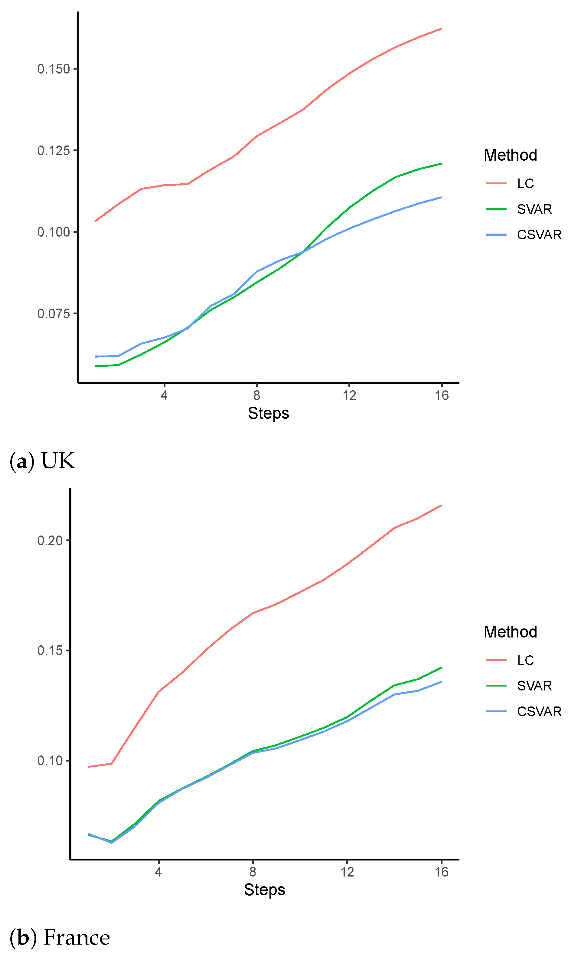
4.2. Out-of-Sample Forecast

Next, we consider the out-of-sample forecasting performance of the proposed CSVAR model. In particular, we compare its forecasting accuracy with those of the Lee-Cater model and the SVAR model. Following Li and Lu (2017) and Feng et al. (2020), the training sample is set to 1950–2000, and the remaining data is used as the test sample. The selected tuning parameters of the SVAR and CSVAR models are reported in Appendix A. For each model, we consider the RMSFEs over age groups and at individual time horizons separately and an overall measure as follows:

$$\begin{array}{cc}\hfill RMSF{E}_x& =\sqrt{{\displaystyle \frac{1}{16}}\sum _{h=1}^{16}{(y_{x,T+h}-{\hat{y}}_{x,T+h})}^2},\hfill \\ \hfill RMSF{E}_h& =\sqrt{{\displaystyle \frac{1}{101}}\sum _{x=0}^{100}{(y_{x,T+h}-{\hat{y}}_{x,T+h})}^2},\hfill \\ \hfill RMSF{E}_{all,h}& =\sqrt{{\displaystyle \frac{1}{101\times h}}\sum _{i=1}^h\sum _{x=0}^{100}{(y_{x,T+i}-{\hat{y}}_{x,T+i})}^2}.\hfill \end{array}$$

(20)

$RMSF{E}_x$ (resp. $RMSF{E}_h$) is the RMSFE averaged over all 16 forecasting steps for age group x (resp. all the 101 ages at forecasting horizon h), and $RMSF{E}_{all,h}$ is the overall measure accounting for all ages and forecasting horizons up to h.

Firstly, $RMSF{E}_{all,h}$ and descriptive statistics of $RMSF{E}_x$ are reported in

Table 1. Summary of RMSE over age groups. For each column, the smallest number is in bold.

	${\mathit{R}\mathit{M}\mathit{S}\mathit{E}}_{\mathit{a}\mathit{l}\mathit{l},16}$	Mean	Std. Dev.	${\mathit{Q}}_1$	${\mathit{Q}}_3$
Panel A: UK
LC	0.1623	0.1454	0.0726	0.0912	0.1935
SVAR	0.1209	0.1056	0.0592	0.0536	0.1571
CSVAR	0.1106	0.1006	0.0463	0.0647	0.1321
Panel B: France
LC	0.2159	0.1661	0.1387	0.0548	0.2601
SVAR	0.1422	0.1210	0.0750	0.0670	0.1594
CSVAR	0.1358	0.1143	0.0736	0.0584	0.1530

, where bold numbers indicate the smallest quantity for each statistic. The mean $RMSF{E}_x$ across all age groups of the CSVAR model is around 44% and 45% (resp. 5% and 6%) smaller than that resulting from the Lee–Carter model (resp. SVAR model) for UK and France, respectively. Moreover, $Q_1$ and $Q_3$ (the first and third quartiles) support that CSVAR model performs reasonably well among the three competing models, and standard deviation of $RMSF{E}_x$ confirms that the $RMSF{E}_x$s of the CSVAR model are more narrowly spread than those of the Lee–Carter and the SVAR models. Finally, as indicated by $RMS{E}_{all,16}$, the overall performance of the proposed CSVAR model is better than the Lee–Carter and the SVAR model for both populations.

Secondly, Figure 5 plots the $RMSF{E}_h$ at individual forecasting horizons ranging from 1 year (2001) to 16 years (2016). Distinct differences among all the three models can be observed, especially at larger horizons. In general, the VAR models consistently outperform the Lee–Carter model in all horizons for both populations. Furthermore, comparing with the SVAR model, $RMSF{E}_h$ of the CSVAR model is smaller in the majority of cases. Finally, with the growth of h (especially from the 8th step onward), the increment in $RMSF{E}_h$ is slower for the CSVAR model than Lee–Carter and the SVAR model, suggesting its better performance in the long run.

4.2.1. Robustness Analysis

To evaluate the robustness of the forecasting results, we perform the out-of-sample forecasting analysis under three major variant settings. Firstly, we follow Li et al. (2013) and Boonen and Li (2017) and model the logged death rates of the five-year ages instead of the single-year groups. Secondly, we consider a shorter training sample of 1970–2000. Finally, instead of crude death rates, we consider the smoothed rates using P-splines (Eilers and Marx 1996), as employed in Hyndman and Ullah (2007). We report the resulting $RMSF{E}_{all,16}$s in

Table 2. Summary of robustness check. For each column, the smallest number is in bold.

	UK			France
	LC	SVAR	CSVAR	LC	SVAR	CSVAR
Five-year groups	0.1674	0.1229	0.1150	0.2240	0.1429	0.1199
1970–2016	0.1507	0.1360	0.1163	0.1916	0.1428	0.1324
Smoothed rates	0.1562	0.1069	0.0987	0.2102	0.1285	0.1140

. It can be seen that the CSVAR model improves the forecasting results of the LC (resp. SVAR) model by at least 30% and 45% (resp. 7% and 8%) for the UK and French data, respectively. Therefore, we conclude that the proposed CSVAR model is able to produce more satisfying forecasting performance compared to the LC and SVAR model under different settings.

4.2.2. The Two-Population Extension

We now investigate the multi-population case by modelling the UK and French data jointly. As discussed at the end of Section 3.2, we consider the situations of a uniform penalty term (CSVAR${}_1$) and individual penalty terms (CSVAR${}_2$). The selected tuning parameters of the SVAR and the two CSVAR models are reported in Appendix A. The results of $RMSF{E}_x$ are summarised in

Table 3. Summary of two-population results. For each column, the smallest number is in bold.

	${\mathit{R}\mathit{M}\mathit{S}\mathit{E}}_{\mathit{a}\mathit{l}\mathit{l},16}$	Mean	Std. Dev.	${\mathit{Q}}_1$	${\mathit{Q}}_3$
Panel A: UK
LL	0.1241	0.1053	0.0660	0.0530	0.1435
SVAR	0.1207	0.1052	0.0594	0.0512	0.1569
CSVAR${}_1$	0.1159	0.1019	0.0555	0.0536	0.1354
CSVAR${}_2$	0.1110	0.1012	0.0459	0.0666	0.1348
Panel B: France
LL	0.1559	0.1303	0.0860	0.0630	0.1770
SVAR	0.1442	0.1220	0.0773	0.0664	0.1600
CSVAR${}_1$	0.1396	0.1178	0.0754	0.0631	0.1469
CSVAR${}_2$	0.1046	0.0906	0.0526	0.0521	0.1172

, where the Li–Lee model is fitted to replace the Lee–Carter model for comparison. The following observations can be made. First, by jointly modelling the UK and French data, the forecasting results of the Li–Lee model are considerably improved over those of the Lee–Carter model displayed in Table 1. This, however, is not the case for SVAR and CSVAR${}_1$. Although their performances are comparatively better than those of the Li–Lee model for both populations, the forecasting results of the CSVAR${}_1$ model and the SVAR model are less accurate than those of the single-population counterparts. For instance, the $RMSF{E}_{all,16}$ of the CSVAR${}_1$ model increase from 0.1106 and 0.1358 to 0.1159 and 0.1396 for UK and French data, respectively. One possible reason of the reduced accuracy in the two-population case is that the VAR model may produce less accurate forecasts when more irrelevant information is included (Feng and Shi 2018). Therefore, the application of a uniform penalty term may lead to the estimated $\hat{\mathbf{M}}$ and $\hat{\mathbf{B}}$ that poorly reflect the historical mortality pattern of both populations. In contrast, when different penalty terms are allowed, the forecasting results of CSVAR${}_2$ are almost uniformly better than those of the Li–Lee, SVAR, and CSVAR${}_1$ model. Furthermore, compared to the single-population forecasts, CSVAR${}_2$ leads to 23% improvement over the single-population CSVAR model of the French data ($RMSF{E}_{all,16}$ of 0.1046 vs 0.1358). As for the UK data, the forecasts of CSVAR${}_2$ are almost identical to those of the single-population CSVAR model. This may suggest that the UK mortality improvements may provide additional important information in the projection of the French improvements, but not vice versa.

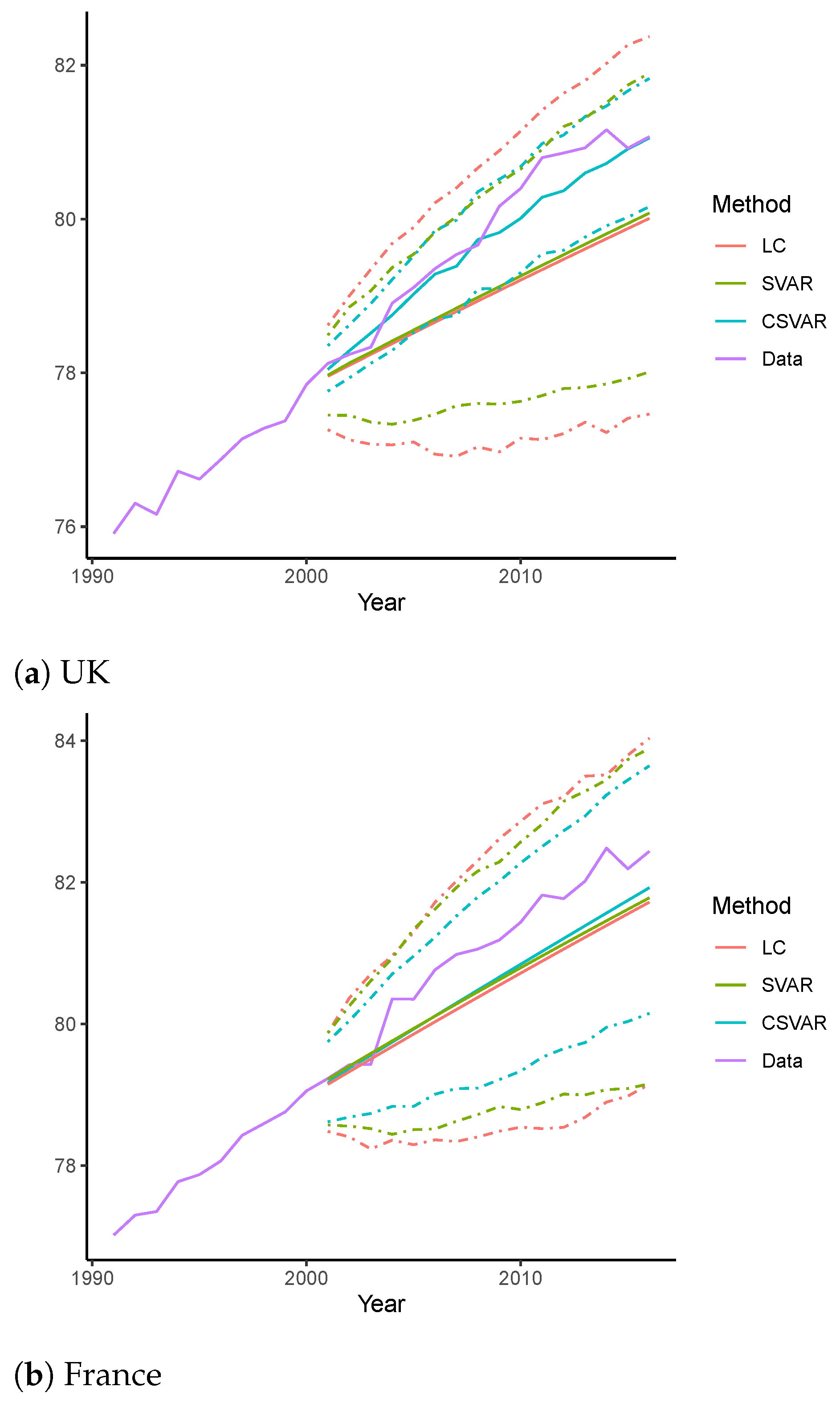
4.2.3. Forecasting of Life Expectancy of Age 0

We now compare the out-of-sample forecasting accuracy of the CSVAR model, the SVAR model, and the Lee–Carter model in terms of life expectancy projection. Again, the life expectancy at birth is used as an illustration. We fit the three models using data from 1950 to 2000, and use the projected log mortality rates to produce ${\hat{e}}_0$ over 2001–2016. The resulting mean forecasts and the 95% prediction intervals are then plotted against the true life expectancies in Figure 6. It can be seen that the ${\hat{e}}_0$s produced by the CSVAR model are uniformly larger than those generated by the Lee–Carter and the SVAR model, especially for the UK data. This is consistent with the age-coherent property of the CSVAR model. More importantly, those forecast ${\hat{e}}_0$ by the CSVAR model are closest to the true values at all horizons for both populations. As for the PIs, all models manage to cover the range of the true $e_0$. In terms of the efficiency, however, the VAR-based models generate narrower PIs than the Lee–Carter model for both populations. In particular, the CSVAR model results in the most efficient interval estimates, with the widths of the UK data almost 50% narrower than those of SVAR.

5. Conclusions

This paper proposes an age-coherent sparse vector autoregressive model to forecast log mortality rates. In particular, we allow the age-specific mortality improvement rates to converge to a universal long-term mean for all ages. The following key results can be drawn from our study. First, the proposed coherent VAR model generates more accurate out-of-sample forecasting results than the Lee–Carter model and the sparse VAR (SVAR) model recently developed by Guibert et al. (2019), as measured by the root-mean-square errors. This result holds for both the uni-sex, single-age UK and the French mortality data for age 0 to 100 with the training sample of 1950 to 2000 and the forecasting period of 2001 to 2016, and is robust when the training sample is shortened to 1970 to 2000 or when five-age mortality data are used instead of the single-age mortality rates. Second, the proposed coherent model retains the attractive advantages of the SVAR model, and has a more flexible parametric structure than the factor-based models, such as the Lee–Carter and the Li–Lee model. In particular, by extending the SVAR model, the proposed model uses the lasso-based algorithm to determine the autoregressive coefficient matrix, and thus the autoregressive matrix is data-driven, rather than based on a prior parameter constraints. Consequentially, the VAR model is able to capture rather general patterns of mortality developments, such as the impact of mortality change of a young age on that of a very old age. Thirdly, by allowing the mortality improvement rates to converge to a universal long-term mean, the proposed model can generate coherent long-term mortality projections, i.e., projected mortality rates at different ages will not diverge in the long-run, such as the spatial-temporal model by Li and Lu (2017). Moreover, by utilizing a hyperbolic decay structure, we allow the speed of convergence to vary with age. Finally, since the number of parameters to be estimated only increase rather moderately with the addition of new populations, the proposed model can be applied to model the joint mortality improvements of multiple populations in an efficient manner. In the multi-population case, projected mortality rates are coherent both on the age and the population dimension. A two-population illustration is made using the UK and French data.

In this paper, we focus on the age-coherent extension of the SVAR model developed by Guibert et al. (2019). However, the proposed age-coherent extension is rather general and applicable to more VAR specifications, such as VAR models with a moving average structure or stochastic volatility. In the future, it would be interesting to explore the age-coherent mortality projections based on more general VAR specifications.

References

1. Boonen, Tim J., and Hong Li. 2017. Modeling and forecasting mortality with economic growth: A multipopulation approach. Demography 54: 1921–46. [Google Scholar] [CrossRef]
2. Booth, Heather, Rob J. Hyndman, Leonie Tickle, and Piet De Jong. 2006. Lee–Carter mortality forecasting: A multi-country comparison of variants and extensions. Demographic Research 15: 289–310. [Google Scholar] [CrossRef]
3. Cairns, A. J. G., David Blake, and Kevin Dowd. 2006. A two-factor model for stochastic mortality with parameter uncertainty: Theory and calibration. Journal of Risk and Insurance 73: 687–718. [Google Scholar] [CrossRef]
4. Chang, Le, and Yanlin Shi. 2020a. Dynamic modelling and coherent forecasting of mortality rates: A time-varying coefficient spatial-temporal autoregressive approach. Scandinavian Actuarial Journal 9: 843–863. [Google Scholar] [CrossRef]
5. Chang, Le, and Yanlin Shi. 2020b. Mortality forecasting with a spatially penalized smoothed var model. ASTIN Bulletin: The Journal of the IAA 51: 161–189. [Google Scholar] [CrossRef]
6. Chen, An, Hong Li, and Mark Schultze. 2020. Tail Index-Linked Annuity: A Longevity Risk Sharing Retirement Plan. Available online: https://papers.ssrn.com/sol3/papers.cfm?abstract_id=3664433 (accessed on 1 November 2020).
7. Dowd, Kevin, Andrew J. G. Cairns, David Blake, Guy D. Coughlan, and Marwa Khalaf-Allah. 2011. A gravity model of mortality rates for two related populations. North American Actuarial Journal 15: 334–56. [Google Scholar] [CrossRef] [Green Version]
8. Eilers, Paul H. C., and Brian D. Marx. 1996. Flexible smoothing with B-splines and penalties. Statistical Science 11: 89–102. [Google Scholar] [CrossRef]
9. Feng, Lingbing, and Yanlin Shi. 2017. Fractionally integrated garch model with tempered stable distribution: A simulation study. Journal of Applied Statistics 44: 2837–57. [Google Scholar] [CrossRef]
10. Feng, Lingbing, and Yanlin Shi. 2018. Forecasting mortality rates: Multivariate or univariate models? Journal of Population Research 35: 289–318. [Google Scholar] [CrossRef]
11. Feng, Lingbing, Yanlin Shi, and Le Chang. 2020. Forecasting mortality with a hyperbolic spatial temporal VAR model. International Journal of Forecasting 37: 255–273. [Google Scholar] [CrossRef]
12. Friedman, Jerome, Trevor Hastie, and Rob Tibshirani. 2010. Regularization paths for generalized linear models via coordinate descent. Journal of Statistical Software 33: 1. [Google Scholar] [CrossRef] [PubMed] [Green Version]
13. Gao, Guangyuan, Kin-Yip Ho, and Yanlin Shi. 2020. Long memory or regime switching in volatility? evidence from high-frequency returns on the us stock indices. Pacific-Basin Finance Journal 61: 101059. [Google Scholar] [CrossRef]
14. Guibert, Quentin, Olivier Lopez, and Pierrick Piette. 2019. Forecasting mortality rate improvements with a high-dimensional VAR. Insurance: Mathematics and Economics 88: 255–72. [Google Scholar] [CrossRef] [Green Version]
15. Ho, Kin-Yip, and Yanlin Shi. 2020. Discussions on the spurious hyperbolic memory in the conditional variance and a new model. Journal of Empirical Finance 55: 83–103. [Google Scholar] [CrossRef]
16. Hosking, J. R. M. 1981. Fractional differencing. Biometrica 68: 165–76. [Google Scholar] [CrossRef]
17. Human Mortality Database. 2020. University of California, Berkeley (USA), and Max Planck Institute for Demographic Research (Germany). Available online: https://www.mortality.org/ (accessed on 1 November 2020).
18. Hunt, Andrew, and David Blake. 2018. Identifiability, cointegration and the gravity model. Insurance: Mathematics and Economics 78: 360–68. [Google Scholar] [CrossRef]
19. Hyndman, Rob J., and George Athanasopoulos. 2018. Forecasting: Principles and Practice. Melbourne: OTexts. [Google Scholar]
20. Hyndman, Rob J., Heather Booth, and Farah Yasmeen. 2013. Coherent mortality forecasting: The product-ratio method with functional time series models. Demography 50: 261–83. [Google Scholar] [CrossRef] [Green Version]
21. Hyndman, Rob J., and Md Shahid Ullah. 2007. Robust forecasting of mortality and fertility rates: A functional data approach. Computational Statistics & Data Analysis 51: 4942–56. [Google Scholar]
22. Lee, Ronald, and Lawrence Carter. 1992. Modeling and Forecasting US Mortality. Journal of the American Statistical Association 87: 659–71. [Google Scholar]
23. Li, Hong. 2018. Dynamic hedging of longevity risk: The effect of trading frequency. ASTIN Bulletin: The Journal of the IAA 48: 197–232. [Google Scholar] [CrossRef]
24. Li, Hong, Anja De Waegenaere, and Bertrand Melenberg. 2015. The choice of sample size for mortality forecasting: A bayesian learning approach. Insurance: Mathematics and Economics 63: 153–68. [Google Scholar] [CrossRef]
25. Li, Hong, Anja De Waegenaere, and Bertrand Melenberg. 2017. Robust mean–variance hedging of longevity risk. Journal of Risk and Insurance 84: 459–75. [Google Scholar] [CrossRef]
26. Li, Han, Hong Li, Yang Lu, and Anastasios Panagiotelis. 2019. A forecast reconciliation approach to cause-of-death mortality modeling. Insurance: Mathematics and Economics 86: 122–33. [Google Scholar] [CrossRef]
27. Li, Hong, and Johnny Siu-Hang Li. 2017. Optimizing the lee-carter approach in the presence of structural changes in time and age patterns of mortality improvements. Demography 54: 1073–95. [Google Scholar] [CrossRef] [PubMed]
28. Li, Hong, and Yang Lu. 2017. Coherent forecasting of mortality rates: A sparse vector-autoregression approach. ASTIN Bulletin: The Journal of the IAA 47: 563–600. [Google Scholar] [CrossRef]
29. Li, Hong, and Yang Lu. 2018. A bayesian non-parametric model for small population mortality. Scandinavian Actuarial Journal 2018: 605–28. [Google Scholar] [CrossRef]
30. Li, Hong, and Yang Lu. 2019. Modeling cause-of-death mortality using hierarchical archimedean copula. Scandinavian Actuarial Journal 2019: 247–72. [Google Scholar] [CrossRef]
31. Li, Hong, Yang Lu, and Pintao Lyu. 2018. Coherent Mortality Forecasting for Less Developed Countries. Available online: https://papers.ssrn.com/sol3/papers.cfm?abstract_id=3209392 (accessed on 1 November 2020).
32. Li, Hong, and Yanlin Shi. 2020. Forecasting mortality with international linkages: A global vector-autoregression approach. Available online: https://papers.ssrn.com/sol3/papers.cfm?abstract_id=3700586 (accessed on 1 November 2020).
33. Li, Hong, Ken Seng Tan, Shripad Tuljapurkar, and Wenjun Zhu. 2019. Gompertz law revisited: Forecasting mortality with a multi-factor exponential model. Available online: https://papers.ssrn.com/sol3/papers.cfm?abstract_id=3495369 (accessed on 1 November 2020).
34. Li, Jackie. 2014. A quantitative comparison of simulation strategies for mortality projection. Annals of Actuarial Science 8: 281. [Google Scholar] [CrossRef]
35. Li, Nan, and Ronald Lee. 2005. Coherent mortality forecasts for a group of populations: An extension of the Lee–Carter method. Demography 42: 575–94. [Google Scholar] [CrossRef] [PubMed] [Green Version]
36. Li, Nan, Ronald Lee, and Patrick Gerland. 2013. Extending the lee-carter method to model the rotation of age patterns of mortality decline for long-term projections. Demography 50: 2037–51. [Google Scholar] [CrossRef] [Green Version]
37. Renshaw, Arthur E., and Steven Haberman. 2003. Lee–carter mortality forecasting with age-specific enhancement. Insurance: Mathematics and Economics 33: 255–72. [Google Scholar] [CrossRef]
38. Renshaw, Arthur E., and Steven Haberman. 2006. A cohort-based extension to the Lee–Carter model for mortality reduction factors. Insurance: Mathematics and Economics 38: 556–70. [Google Scholar] [CrossRef]
39. Shi, Yanlin. 2020. Forecasting mortality rates with the adaptive spatial temporal autoregressive model. Journal of Forecasting. [Google Scholar] [CrossRef]
1.
A maximum likelihood method may also be employed to calibrate the parameters (Renshaw and Haberman 2003).
2.
Note that the choice of the length of test sample (one fifth) is common among existing studies. Adopting other popular alternatives such as the last third, fourth and tenth sample will lead to robust results.
Figure 1. Demonstrations of the inversed Epanechnikov kernel.
Risks 09 00035 g001
Figure 2. Uni-sex mortality data of the UK and France of age 0–100 and year 1950–2016.
Risks 09 00035 g002
Figure 3. Projected and actual log central death rates: 2016 vs. 2100.
Risks 09 00035 g003
Figure 4. Mean forecast and the 95% prediction intervals vs. actual life expectancy at bitrh: 2001–2100.
Risks 09 00035 g004
Figure 5. RMSE over forecasting steps.
Risks 09 00035 g005
Figure 6. Forecast vs actual life expectancy at age 0: 1991–2016.
Risks 09 00035 g006