Article

Common Factor Cause-Specific Mortality Model

by
Geert Zittersteyn
1 and
Jennifer Alonso-García
2,3,4,*
1
ILX, Linnaeusstraat 2A, 1092 CK Amsterdam, The Netherlands
2
Department of Mathematics, Université Libre de Bruxelles, Boulevard du Triomphe, B-1050 Bruxelles, Belgium
3
ARC Centre of Excellence in Population Ageing Research (CEPAR), UNSW Sydney, 223 Anzac Pde Kensington, Sydney, NSW 2033, Australia
4
Netspar, Warandelaan 2, 5037 AB Tilburg, The Netherlands
*
Author to whom correspondence should be addressed.
Risks 2021, 9(12), 221; https://doi.org/10.3390/risks9120221
Submission received: 18 October 2021 / Revised: 25 November 2021 / Accepted: 1 December 2021 / Published: 3 December 2021
(This article belongs to the Special Issue Longevity Risk Modelling and Management)

Abstract

:
Recent pension reforms in Europe have implemented a link between retirement age and life expectancy. The accurate forecast of life tables and life expectancy is hence paramount for governmental policy and financial institutions. We developed a multi-population mortality model which includes a cause-specific environment using Archimedean copulae to model dependence between various groups of causes of death. For this, Dutch data on cause-of-death mortality and cause-specific mortality data from 14 comparable European countries were used. We find that the inclusion of a common factor to a cause-specific mortality context increases the robustness of the forecast and we underline that cause-specific mortality forecasts foresee a more pessimistic mortality future than general mortality models. Overall, we find that this non-trivial extension is robust to the copula specification for commonly chosen dependence parameters.

1. Introduction

Since 1950, the period life expectancy of Dutch males (females) at age 65 has increased from 14.39 years to 18.97 (14.94 to 21.49) in 20171. Even more remarkably, for males at retirement age (assumed 65), life expectancy has increased by approximately 2 years over the past decade. According to Actuarieel Genootschap (2018), life expectancy is only expected to rise further to a predicted level of approximately 22 and 25 years in 2050 for males and females, respectively. Recent pension reforms in Europe have implemented a link between retirement age and life expectancy (Alvarez et al. 2021; OECD 2015). This has led to researchers focusing on accurate mortality modelling within a pension context (Ayuso et al. 2021). It becomes clear that the accurate forecast of life tables and life expectancy is paramount for governmental policy and financial institutions.
In the past fifty years, mortality shocks have not been extremely dramatic. Nevertheless, we could think of several hypothetical scenarios where mortality could be heavily altered, such as a deadly viral epidemic2, or vice versa, a solution to a major deadly disease. Such eventualities are difficult to account for beforehand, but could potentially severely affect our current predictions of future mortality rates. To address these scenarios, it becomes natural to use cause-of-death mortality modelling to study increases or decreases for certain diseases.
In practice, the most prominent methods for forecasting mortality in the Netherlands or elsewhere focus on general mortality and its trend over time. The models used vary from the seminal work of Lee and Carter (1992) to multi-population3 extensions such as the one introduced by Li and Lee (2005). Whereas the original Lee–Carter model estimates and forecasts are solely based on the past observed mortality of an individual population, the Li–Lee model incorporates a so-called common factor which is an additional variable translating the shared effects of other comparable populations. Through this method, data are increased and parameter estimates become less sensitive to the incidental deviation of individual mortality. In addition, the undesirable property of forecast divergence for individual populations is countered. However, Enchev et al. (2017) highlighted that the model in Li and Lee (2005) might have had robustness issues despite being a well performing model 4. Despite its shortcomings, the common factor model relies on a data increase to provide more robust estimates, thus becoming the new standard to produce mortality projections in Belgium and the Netherlands (Antonio et al. 2017).
Li and Lee (2005), in their seminal specification, did not incorporate cause-of-death mortality. However, the accumulation of these established facts motivates our research into cause-specific mortality that might be more capable to predict future mortality in case of unexpected events regarding specific causes of death. In doing so, choices need to be made regarding how causes-of-death are linked. A rich literature relies on copulas to model this dependence. Furthermore, the assumption of mortality convergence may be too restricting in the short-term mortality dependence between co-integrated populations, in particular in the context of catastrophic events such as a pandemic. To overcome this, Zheng and Klein (1995) went beyond the dependence of competing risks5 and proved that under an assumed copula function, competing risk mortality data are sufficient to derive the marginal survival distributions of separate risks. However, they acknowledged that the choice of a copula function may seem too restrictive, even though their results are quite robust to this choice. Chen et al. (2015) presented a novel factor copula approach to model dependence between populations. This straightforward copula was used to model the dependence of mortality improvements for six developed countries and was applied to mortality-linked securities pricing and hedging. It provides flexibility in which additional factors can be added to account for cohort or socio-economic information. However, this is left for future research. More recently, Li and Lu (2019) created a cause-specific mortality model using hierarchical and non-hierarchical Archimedean copulae. The underlying model formulation is the Lee–Carter single population model. Through the copula, the dependence between different cause-specific mortalities is captured. Their research underlines the importance of evaluating model uncertainty, since they show that differences between at first glance similar models can be significant under certain circumstances. We extended the Li and Lee (2005) model by incorporating cause-specific mortality into its structure. For this, we used the Archimedean copula to model the dependence of cause-specific mortality as described in Li and Lu (2019). We used this model to forecast future Dutch mortality based on past observed cause-specific mortality for the Netherlands and 14 European countries6.
It should be noted that not all authors use copula theory to model dependence. Indeed, Boumezoued et al. (2018) assumes the independence of cause-specific mortality in their research into the effects of a reduction in cause-specific mortality for demographic composition in France. This assumption allows one to directly estimate the marginals from the data. Arnold and Sherris (2015) used vector error correlation models for the modelling of this dependence. With their findings, they underlined the presence of a relationship between mortality from different causes. Furthermore, they warned that inference for cause-specific mortality for one country based on conclusions from another may be deceptive. In the recent research conducted by Lyu et al. (2020) on cause-of-death mortality, the authors used a two-step convergence test to capture the cause-specific mortality dynamics both between countries and between causes which yields a better out-of-sample performance than earlier models. A recent paper by Li et al. (2019) utilises clustering methods to group different causes of death. Via a reconciliation approach, the authors were able to model coherent mortality using all sub-groups. This means that the aggregate, clustered and cause-specific mortality are considered in the forecasting procedure. The model performed better in comparison to the general mortality model and the bottom-up approach. Furthermore, the model still takes into account the interdependence of causes. This ensures the integration of competing risk effects for cause-removal analysis, leading to more rational results.
Our multi-population with a cause-of-death and copula dependence structure extends the models of Li and Lee (2005) and Li and Lu (2019) and is general enough to extend the model of Lyu et al. (2020) who studied multi-population cause-of-death models with ad hoc dependence structures. We found that cause-specific mortality models forecast a much lower life expectancy with respect to general mortality models amounting to up to 3 years by 2060, the end of our forecasting period. Including a common factor in the cause-specific mortality context shows more resistance to the short-term effects within Dutch mortality. This proves the increased robustness of our forecasting model with respect to a single population model. Overall, we find that this non-trivial extension is robust to the copula specification for commonly chosen dependence parameters.
This paper is structured in the following way: Section 2 outlines the steps and methods used to create the conclusive cause-specific mortality forecasting model; Section 3 describes the data set and the needed modifications to render it suitable to our study; Section 4 discusses the results and the last section concludes and discusses the venues for future research.

2. Methodology

The Lee–Carter model (henceforth the LC model) is considered the “leading statistical model for mortality” (Deaton and Paxson 2004). However, in their article, Girosi and King (2007) addressed its drawbacks. The LC model performs strongly for individual populations (Lee and Carter 1992). However, an undesired feature of the model is that mortality forecasts of different single populations potentially diverge in situations for which diverging mortality trends are not expected based on past observations (Lee and Nault 1993; Tuljapurkar et al. 2000).
Moreover, research shows a more rapid decrease in mortality levels in populations with a lower life expectancy in comparison to the on average longer living populations (Oeppen and Vaupel 2002). In other words, in countries with a relatively low expected lifespan, life expectancy rises more quickly. This has been pointed out in research conducted by White (2002) for developed countries and can easily be observed on continental and on a worldwide scale. These observations suggest the convergence of life expectancy internationally in the past, since most countries with low life expectancy catch up with long-living countries.
From a perspective of ever-increasing interconnection between countries and regions caused by globalisation, Li and Lee (2005) have extended the Lee and Carter (1992) model by incorporating the data of closely connected and socioeconomically similar populations. The Li–Lee model (LL model) first determines the collective main trend of the group of populations as a whole by applying the so-called common factor method. Then, they analyse the unique dissimilarities of an individual population on a short or medium horizon. This is done in order to model the historical deviation of the single population with respect to the common tendencies of the entire group. The combination of both stages, results in a mortality model that asserts a non-diverging relation between populations in the long run while retaining the explanatory power of the short/medium-term variation of mortality for individual populations7. We will specify the specifics of our LL model in Section 2.3 after specifying how we address the cause-of-death mortality component.

2.1. Cause-of-Death Mortality

The objective of this research was to model cause-specific mortality. To do so, we needed to use the crude and net cause-of-death mortality. The crude mortality is the observed probability of death due to a certain cause for a population. It is possible to more thoroughly investigate mortality by looking beyond this factual observed mortality. Specifically, when an individual dies as a result of one disease, the same individual obviously cannot suffer death from another cause. Consequently, the crude mortality underestimates or is equal to the real underlying mortality of the specific disease. This definition of mortality that takes other potential causes of death into account is called net mortality. In the next part of this section, we mathematically provide how we derive these mortality variables.

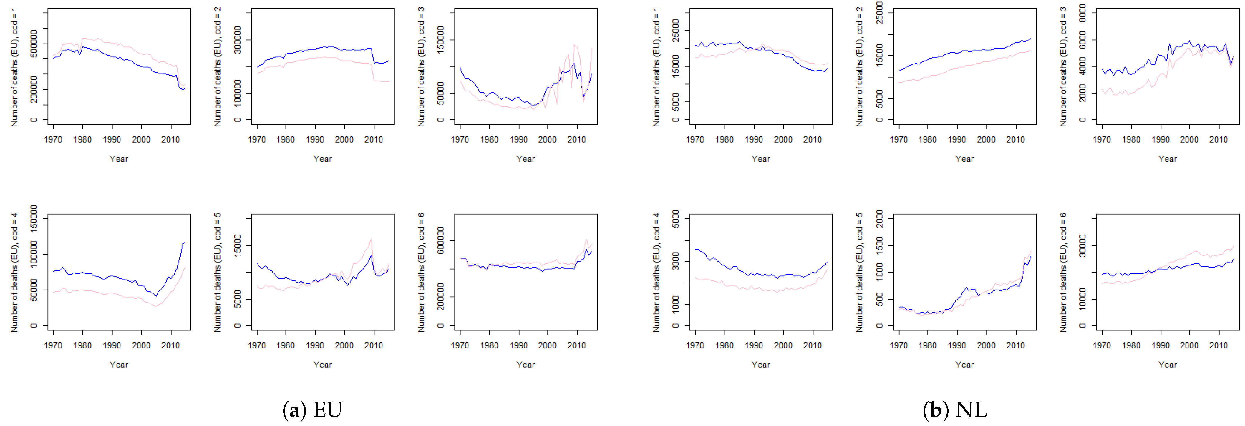
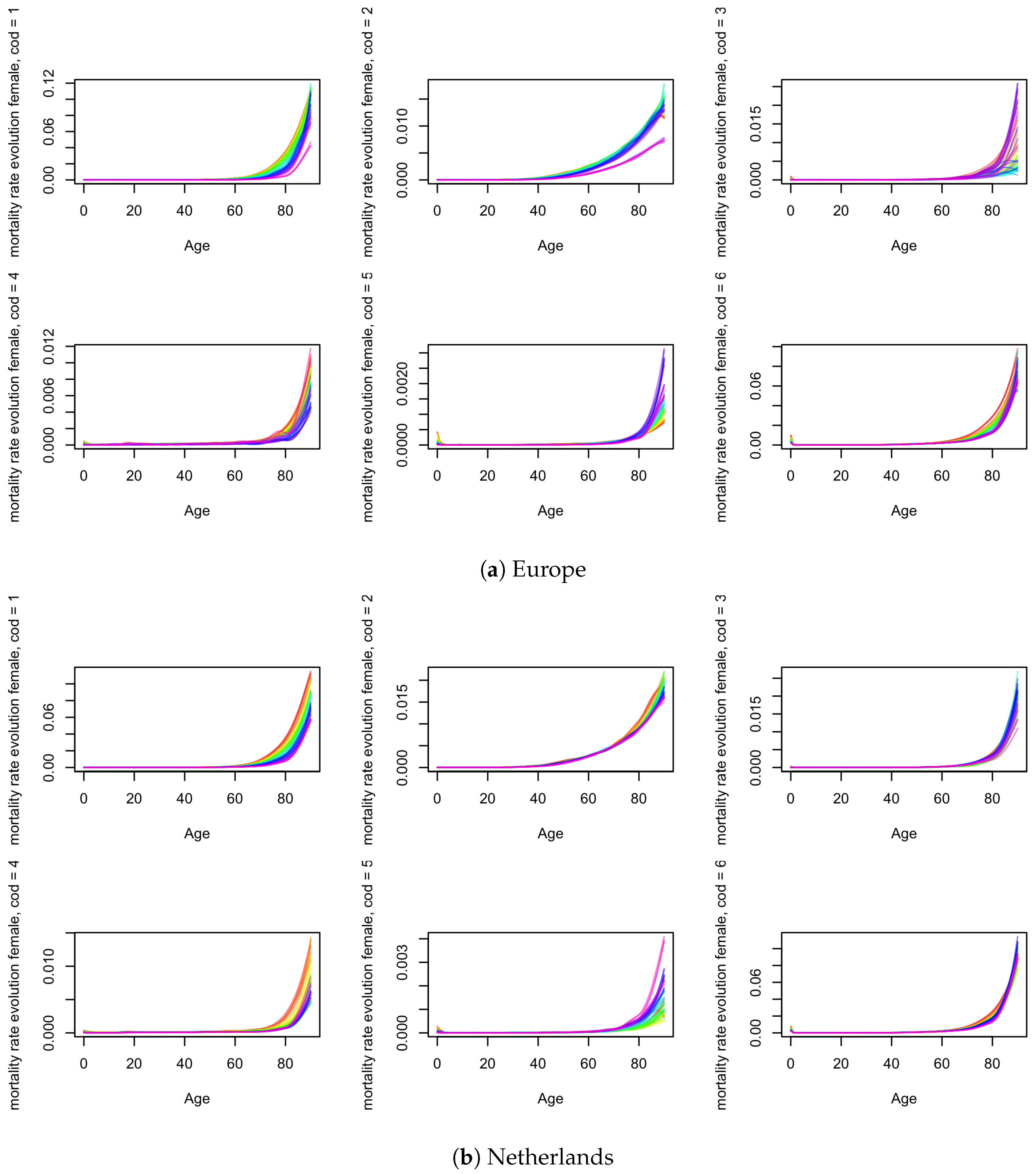
2.1.1. Crude Mortality

We regard both EU and NL data as homogeneous populations (population is denoted as i) with independent and identical distributed lifetimes X i = min ( X i 1 , , X i z ) , where X i c is the age at death due to cause c. Then, we let ( X i , C ) represent the time of death and the corresponding cause of death, C { 1 , , z } . Under the assumption of independence between causes of death, we find in the literature (Boumezoued et al. 2018; Li and Lu 2019) the crude cause-of-death mortality for age x defined as
μ c ( x ) = lim u 0 P [ X i x + u , C = c | X i > x ] u .
Since our data are discrete, we define the observed crude cause-of-death as
m i c ( x , t ) = D i c ( x , t ) E i ( x , t ) .
where the age group of age x of population i in year t has a size E i ( x , t ) . The same year, this group experiences D i c ( x , t ) deaths from cause c. All independent mortality rates cumulatively describe the general mortality of the population:
m i ( x , t ) = c = 1 z m i c ( x , t ) ,
with the corresponding overall survival function:
S i ( x , t ) = exp ( k = 0 x c = 1 z m i c ( k , t ) ) .

2.1.2. Net Mortality

For the determination of net mortality, we turn to the joint distribution of X i . We follow the specification as given by Li and Lu (2019). The joint survival probability is given by
S ( x 1 , , x z ) = P [ X 1 > x 1 , , X z > x z ] .
Then, for the cause of death c, we define the net cause-specific mortality of X i c in year t and age x as
λ c ( x , t ) = lim u 0 P [ X c x + u , C = c | X c > x ] u
and accordingly, we subsequently obtain the net survival function of X i c in a discrete context. The net survival function describes the probability of having survived a specific cause of death at age x during period t as follows:
S c ( x , t ) = exp ( k = 0 x λ c ( k , t ) ) = P [ X c > x , X { C } c > 0 ] .

2.2. Competing Risk

As we determined in the literature review, many researchers have previously studied the dependence of cause-specific mortality. The results convince us that it is relevant to incorporate the possible dependence of varying mortality categories. Hence, we will expand on the implemented method to assess the dependence between the separate cause-specific mortality distributions. In our explanation of the procedure, we follow the steps of Li and Lu (2019). Tsiatis (1975) showed that observed data Are insufficient for the identification of the latent dependence structure of cause-of-death mortality and therefore additional constraints are needed. The use of survivor copula is a prevalent method applied to address the dependence.8
For the study of cause-related mortality, we turned to the survivor copula. The survivor copula reveals the dependence of the implicit cause-specific survival functions, denoted by ( S 1 ( X 1 ) , , S z * ( X z * ) ) . We define the cumulative distribution function as follows:
S ( u 1 , , u z * ) = P [ S 1 ( X 1 ) < u 1 , , S z * ( X z * ) < u z * ] ,
where all u c are uniformly distributed, c = c * = { 1 , , z * } . Here, c * is defined as all causes of death except other causes. Other causes will be regarded as independent censoring. Reversely, from Equation (8), we obtain:
P [ X 1 > x 1 , , X z * > x z * ] = S ( S 1 ( x 1 ) , , S z * ( x z * ) ) ,
with positive x c and c = c * . We determined an expression for the joint distribution of the lifespan which depends on the specification of joint distribution function S and the net survival function S c ( X c ) . Since the cause-specific survival functions have uniform marginals, S qualifies by definition as a copula and is henceforth referred to as the survivor copula.
Li and Lu (2019) considered the approach performed in Carriere (1994) to solve the system straight from data using the nonlinear partial differential equations. In their paper, they indicated a major drawback of this approach, which is the lack of an analytical solution. In conformance with this argumentation, we also opted for a closed-form expression.
First, we assumed a joint Archimedean survivor copula which applies to the random survival variables ( X 1 , , X z * ) . We can now rewrite Equation (9) using the formulation of the Archimedean copula introduced by Ling (1965):
P [ X 1 > x 1 , , X z * > x z * ] = S ( S 1 ( X 1 ) , , S z * ( X z * ) ) = ψ ( ψ 1 ( S 1 ( x 1 ) ) , , ψ 1 ( S z * ( x z * ) ) ) ,
with positive x c , c = c * . The expression ψ ( · ) implies the copula generator function which satisfies the necessary and sufficient condition of d-monotonicity (McNeil et al. 2009). Similarly to Li and Lu (2019), we will discuss two variations of the Archimedean copula family:
Frank copula : ψ ( t ) = 1 θ l n ( 1 + e t ( e θ 1 ) ) , where θ 0 .
Clayton copula : ψ ( t ) = 1 ( 1 + t ) θ , where θ 0 .
In these equations, θ denotes the dependence coefficient. For θ = 0 , the copulas above equate to the independence copula. When an independence copula is assumed, the net mortality value equals crude mortality.9
Under the assumption of a known pre-specified Archimedean copula, we can proceed with the direct calculation of the net survival functions from the observed data. First, we derived the crude cause-specific mortality from the data. We plugged these into the discrete formulation of the net survival function established by Rivest and Wells (2001); Wang (2012) obtaining the following expression of the marginal survival distribution for population i, cause c, age x and year t:
S i c ( x , t ) = ψ s = 0 x exp u = 0 s k = 1 z * m i k ( u , t ) ψ ψ 1 exp u = 0 s k = 1 z * m i k ( u , t ) · m i c ( s , t ) ,
where ‘∘’ is the notation used for expressing the composition of functions. Conversely, for age x and for known S i ( x , t ) (through Equation (4)), this equation becomes:
m i c ( x , t ) = ψ 1 ( S i c ( x , t ) ) s = 1 x 1 S i ( s , t ) ψ ψ 1 S i ( s , t ) · m i c ( s , t ) S i ( x , t ) ψ ψ 1 S i ( x , t ) .
The cause-specific mortality at age 0 can be derived as
m i c ( 0 , t ) = ψ 1 ( S i c ( 0 , t ) ) S i ( 0 , t ) ψ ψ 1 S i ( 0 , t ) .
A full comprehensive overview of the steps taken to derive Equation (14) in combination with (15) is given in Appendix A, Equation (7). Now that the marginal survival functions are known, we can readily determine the net mortality by solving:
λ i c ( x , t ) = ln S i c ( x , t ) S i c ( x 1 , t ) .
Note again that for an assumed θ = 0 , the net mortality will equal the crude mortality for both mentioned copulas.

2.3. Model Estimation
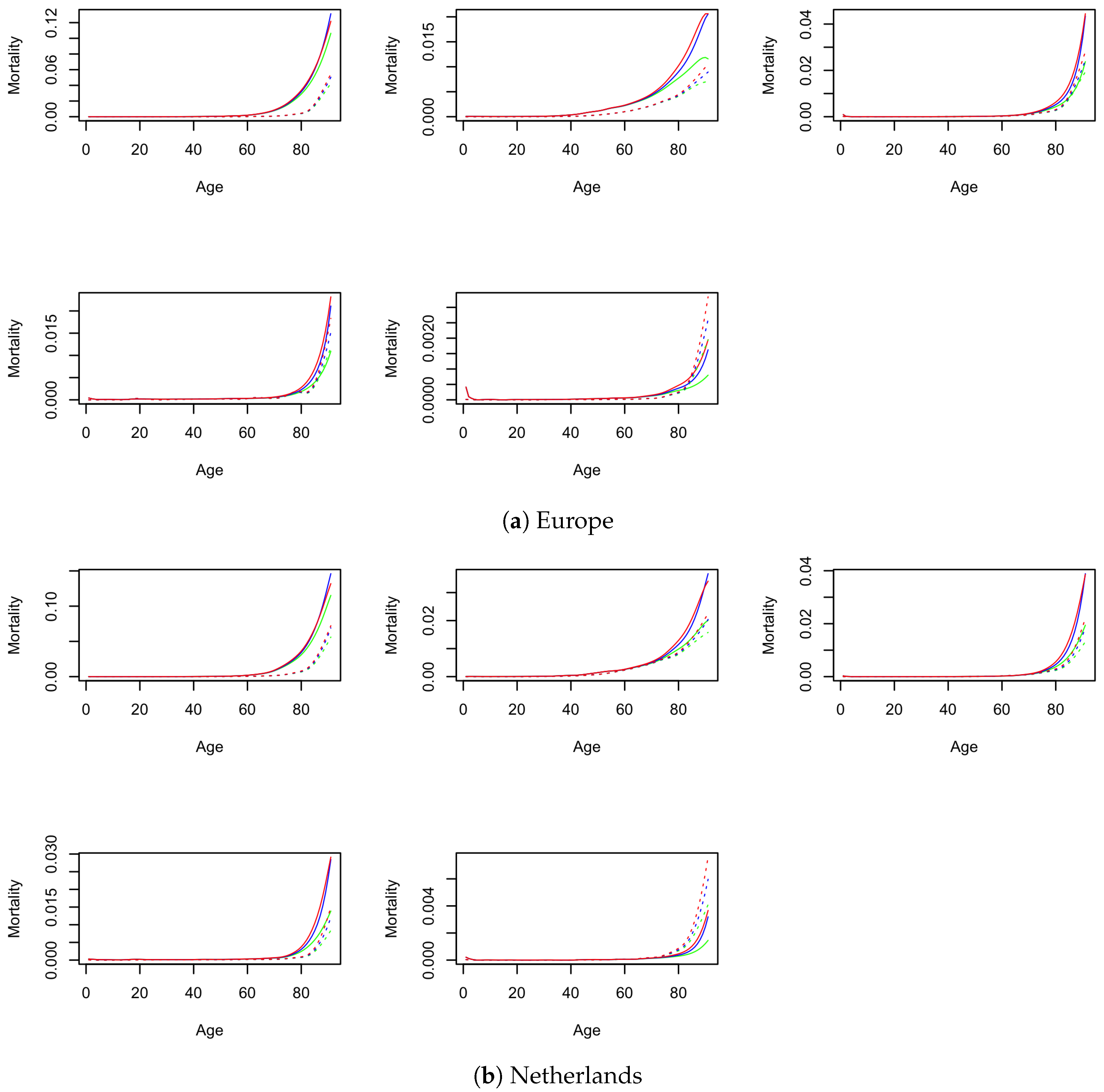
The construction of the Li and Lee (2005) model can be described in two stages. For the first stage, we define the observed mortality for population i:
m i ( x , t ) = D i ( x , t ) E i ( x , t ) .
D i ( x , t ) denotes the amount of deaths observed in year t for people aged x. E i ( x , t ) describes the corresponding age group exposure, i.e., the population size per age. For the observed matrix containing the historical mortality rates m i ( x , t ) for age x and during the period t = [ 1 , T ] , the LC model is described as follows:
l n ( m i ( x , t ) ) = a i ( x ) + b i ( x ) k i ( t ) .
where the coefficient a i ( x ) denotes the general age-specific mortality constant. The responsiveness of the mortality rate of a certain age group x to changes of time dependent mortality development is given by the coefficient b i ( x ) or, in other words, the coefficient b i ( x ) denotes the sensitivity across age groups to variation in the time-varying parameter k i ( t ) . Due to the fact that the model is underdetermined (the number of unknown parameters exceeded the number of equations), the authors impose two constraints:
x b i ( x ) = 1 and t k i ( t ) = 0 ,
which in turn directly imply that a i ( x ) equals the average log mortality rates over time.
For the second stage, it was required that all populations within the group have identical b i ( x ) and k i ( t ) , denoted by B ( x ) and K ( t ) , respectively. Furthermore, each population i has an age-specific effect A i ( x ) which is allowed to vary among the group members and are thus estimated individually. This is done because this variable is a constant and will therefore not lead to divergence. The ensuing common factor equation is equivalent to the LC model with the replaced variables:
l n ( m i C F ( x , t ) ) = A i ( x ) + B ( x ) K ( t )
In addition to the common factor, Li and Lee (2005) pinpoints the individual mortality effects for population i. To put it differently, we need to model the residuals from the common factor Equation (20) for population i using the age-dependent variable b i ( x ) and the time-varying term k i ( t ) . The resulting extended common factor model is specified as follows:
l n ( m i ( x , t ) ) = a i ( x ) + B ( x ) K ( t ) + b i ( x ) k i ( t ) .
In practice, we fit the model within a Poisson framework as in Enchev et al. (2017) and Brouhns et al. (2002). We denoted by d i c ( x , t ) the actually observed number of deaths for population i by cause of death c and let D i c ( x , t ) be the random variable for the amount of deaths at time t for age x. Similarly to Brillinger et al. (1986), we assume:
D i c ( x , t ) P o i s s o n ( λ i c ( x , t ) E i ( x , t ) ) ,
where E i ( x , t ) represents the exposure and λ i c ( x , t ) represents the age-specific net mortality intensity for cause c, at age x and time t. Then, in turn, the likelihood function can be defined as follows:
L i c ( x , t ) = x t ( λ i c ( x , t ) E i ( x , t ) ) D i c ( x , t ) · e λ i c ( x , t ) E i ( x , t ) D i c ( x , t ) ! .
Following Brillinger et al. (1986), we derive the log-likelihood function from (23):
i c ( x , t ) = x t [ D i c ( x , t ) · ln { λ i c ( x , t ) E i ( x , t ) } λ i c ( x , t ) E i ( x , t ) ln { D i c ( x , t ) ! } .
The maximum likelihood estimation for our model consists of two stages which are described in Appendix B. The parameter estimations are performed for both sexes separately. We denote the resulting parameter estimates θ ^ c , g { A ^ e u c , g ( x ) , B ^ e u c , g ( x ) , K ^ e u c , g ( t ) , a ^ n l c , g ( x ) , b ^ n l c , g ( x ) , k ^ n l c , g ( x ) } , for g = { male , female } and all causes c.

2.4. Forecast

The goal of the model estimation presented is forecasting future mortality. In this section, we will focus on the time-dependent variables of our model, denoted by K i c , g ( t ) and k i c , g ( t ) . In the previous section, we fitted the parameters using MLE, including those describing the two time-dependent variables. The resulting subset of estimates θ ^ c , g , K c = { K ^ e u c , M ( t ) , k ^ n l c , M ( t ) , K ^ e u c , F ( t ) , k ^ n l c , F ( t ) } were re-estimated using the time series analysis of the following equations using an ARIMA (p,d,q) process. We used the same specification as Li and Lee (2005) who suggested an ARIMA (0,1,0) and an ARIMA (1,0,0)10 model for K i c , g ( t ) and k i c , g ( t ) , respectively:
K ( t ) = K ( t 1 ) + ρ + η ( t ) , η ( t ) N ( 0 , σ η ( t ) 2 ) ,
k i ( t ) = c i + ω i k i ( t 1 ) + ϵ i ( t ) , ϵ i ( t ) N ( 0 , σ ϵ i ( t ) 2 )
where ρ denotes the constant drift coefficient which is straightforwardly estimated by ρ ^ = ( K ^ ( T ) K ^ ( 1 ) ) / ( T 1 ) , as t = [ 1 , T ] is the range of years used for the estimation. Furthermore, c i is a constant, ω i 1 and ϵ i ( t ) N ( 0 , σ ϵ i ( t ) 2 ) . The resulting system of time series equations for K c were simultaneously estimated using the method of seemingly unrelated regressions (SURs) (Zellner 1962). This method allows information acquired from one equation to be used by the estimation of another, by assuming the error terms to be correlated. This possibly increases efficiency and can be supported by the idea that shocks in mortality for a specific age in a specification year for male and female will probably be strongly correlated. Finally, we let the set of errors { η e u c , M ( t ) , ϵ n l c , M ( t ) , η e u c , F ( t ) , ϵ n l c , F ( t ) } follow a four-dimensional normal distribution with mean 0 and covariance matrix H c . To forecast K c , we assumed the time series error to be none. From these forecasts, we in turn can derive the crude mortality forecasts for the Netherlands m n l c ( x , t ) by applying (14).

2.5. Old Ages

The data set we used includes a maximum age of 90, whereas the eventual data set we opted to use ages up to and including 120. Therefore, similarly to Antonio et al. (2017), we used the theory of Kannisto (1994) as the extrapolation method for the ages over the maximum age available in the data. We wanted to estimate the mortality for the ages x o = { 90 , , 120 } . This estimation was based on mortality of ages x y = { 80 , , 90 } . This is executed by performing a logistic regression on the n = 11 observations x y :
m c ( x o , t ) = f k = 1 n w ( x o , k ) · f 1 m c ( x k y , t ) ,
where f ( · ) and f 1 ( · ) are defined as
f ( α ) = ( 1 + e α ) 1 ,
f 1 ( α ) = ln 1 α 1 .
The weights w ( x , i ) are defined in the following fashion:
w ( x , i ) = 1 n + ( x i y x ¯ y ) ( x x ¯ y ) j = 1 i ( x j y x ¯ y ) 2
= 1 11 + ( x i y 85 ) ( x 85 ) 110 .
A short overview of all steps taken is shown in the Supplementary material Section S.1.

2.6. Population Dynamics

The objective of simulating the population dynamics is to be able to concretely assess the consequences of model uncertainty and of cause-specific mortality shocks on the population. Since our goal was to analyse the implications of our model, we opted for a simulation method that was more stable since it relies on one forecast of demographic variables11 as the basis instead of on random variables. For this, we used CBS data12. The resulting data set consists of the following variables for the Netherlands:
  • M g ( x , t ) : net migration for males and females (g) for age x (from 0 to 99 years old) in year t. We assume migration for ages 100 to 120 to be zero;
  • B g ( t ) : total life births for males and females (g) in year t;
  • m n l g ( x , t ) : the total crude mortality intensity for Dutch males and females (g) aged x in year t. This variable is obtained through Equation (3). We assumed mortality for individuals older than 120 in year t to equal that of a 120-year-old.
  • E g ( x , 2016 ) : the exposure for males and females on the first day of 2016, aged x (from 0 to 99 years old). We assume the first period exposure for ages above 99 to equal zero.
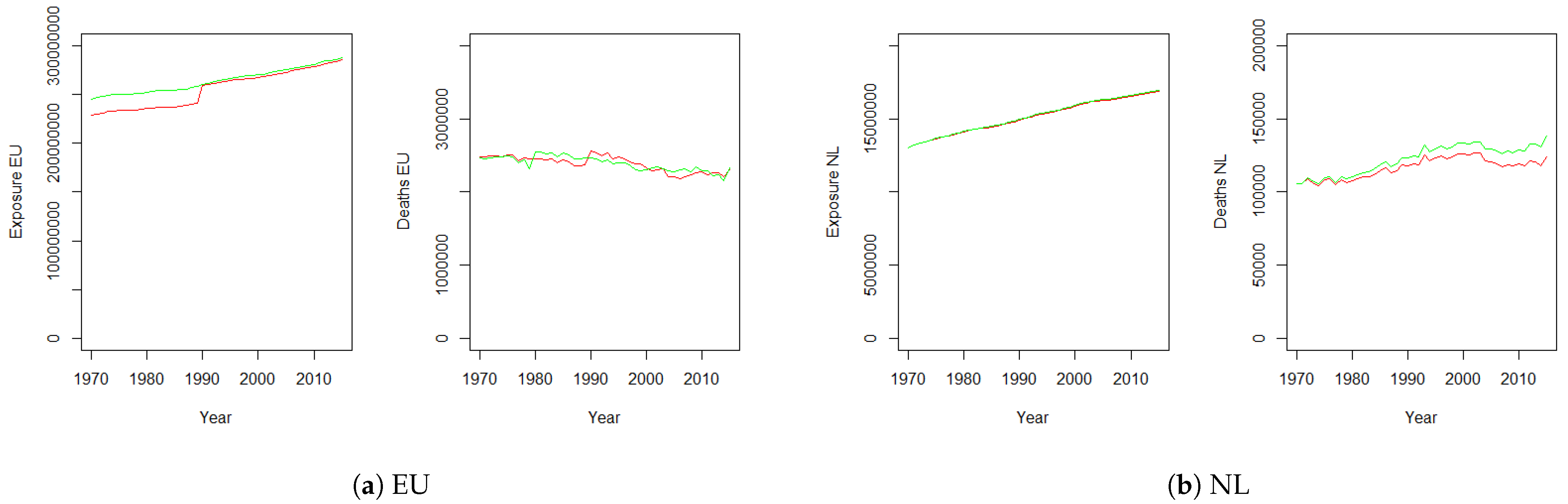
Before we proceed, we transform the crude mortality intensities into the probability of death q n l g ( x , t ) for age x in year t:
q n l g ( x , t ) = 1 e m n l g ( x , t ) .
We will give a mathematical formulation of the iterative modelling procedure below for t = ( 2016 , , 2059 ) :
( 1 ) D g ( x , t ) = q n l g ( x , t ) + q n l g ( x + 1 , t ) 2 · E g ( x , t ) , ( 2 ) D ˜ g ( x , t ) = 2 D g ( x , t ) 2 , ( 3 ) E g ( x , t + 1 ) = max { 0 , E g ( x 1 , t ) D ˜ g ( x , t ) + M g ( x , t ) } , for x 0 , ( 4 ) E g ( 0 , t + 1 ) = B g ( t ) .
After having simulated the Dutch population and its corresponding composition, we will compare the model outcomes using three different variables. Similarly to Boumezoued et al. (2018), we denote the ratio of individuals aged 65 and older and individuals aged between 15 and 65, commonly referred to as the dependency ratio:
d t = E ( [ 65 , 120 ] , t ) E ( [ 15 , 64 ] , t ) .
The second and third variable used for model comparison are two variations of life expectancy, namely the period and cohort life expectancy. We will compare these measures for several varying cause-of-death circumstances. The method used for this in Boumezoued et al. (2018) is the multiplication of the crude mortality values by some factor r. We will apply a similar method, only in our case, the multiplication will be applied to the net mortality intensities instead of their crude compliments. Net mortality is reduced for r < 1 and increased for r > 1 .

3. Data

The common factor model relies on a data increase to provide more robust estimates. Hence, the choice of sub-population is a careful one. As in Antonio et al. (2017), our choice relies on the gross domestic product (GDP). Indeed, Boonen and Li (2017) gives an insight into the close relation between mortality forecasts and GDP levels by including the logarithm of the real GDP as an explanatory variable. The inclusion proves advantageous for mortality estimation in general, as both in-sample fit as well as out-of-sample forecast performance improve with respect to the original Li–Lee model.
The inclusion of 14 countries is essential for the model as it creates additional model stability and the estimates become less sensitive to random shocks of Dutch mortality. The same rationale applies for the cause-specific case. This section provides the steps to obtain data suitable to our study.
The data set containing cause-of-death mortality data for Europe used for the common factor part of the competing risk LL model was obtained from the World Health Organization (WHO) Mortality Databass13. This data set contains mortality data in the form of yearly number of deaths and mid-year population levels, ranging from the years 1950 to 2017. The data set for the Dutch cause-of-death mortality and mid-year population, from now on referred to as NL, was acquired from StatLine of Centraal Bureau voor de Statistiek (CBS)14. The same cause-of-death specifications as for the WHO Mortality Database hold. We chose to use the CBS data instead of the WHO data since, unlike the WHO data set, this data set does not involve all shortcomings described in Section S.2.
We selected the following countries based on their GDP as in Antonio et al. (2017) and included the data from 1970 to the latest year available for all countries, namely 2015. This allows us to better compare our model to existing ones based on the same database. The countries are, in alphabetical order: Austria, Belgium, Denmark, Germany15, Finland, France, Iceland, Ireland, Luxembourg, The Netherlands, Norway, Sweden, Switzerland and the United Kingdom.
For the purpose of ensuring the consistency of the cause-of-death indication between countries, the mortality database provided by the WHO employs cause classification according to the guidelines of the International Classification of Diseases (ICD), provided by WHO since 1948. The most recent revision of the classification guidelines, ICD-10, was endorsed by the Forty-third World Health Assembly in 1990 and is now used by all the European countries we included in our research. For these countries, four different classifications have been used during the period of 1970–2017. These are namely ICD-7, ICD-8, ICD-9 and ICD-10. Since for all the different countries these classification guidelines were adopted in different years, we must for now process and refine each country individually. We explain this in detail in the Supplementary material Section S.2.
Through transformations, we made a data set comparable to that used by Antonio et al. (2017), as shown in Figure 1a,b. The biggest difference is caused by the inclusion of the combination of West and East Germany, which causes the jump in the red line between 1989 and 1990. Moreover, we see that for both data sets, the mortality levels do not correspond one to one. In the EU case, the levels fluctuate around those utilised by Antonio et al. (2017), but overall, they do not significantly deviate. In the NL case, we see that over the years the level of mortality in our data set increasingly exceeds that of Antonio et al. (2017). Some of this we can account for by the transformation introduced in Equation (S2), but most of the difference in slope is inherent to the cause-of-death data set that we used. In addition, we see that the population size of our NL data set also increasingly exceeds its reference level, which compensates for the mortality surplus in terms of deaths per exposure ratio. Figure 2 illustrates the level of deaths over the time period 1970–2015 per cause of death for the ultimate data sets. For the time period of 1970–2015, the contribution of each cause to total mortality is presented in Table 1.

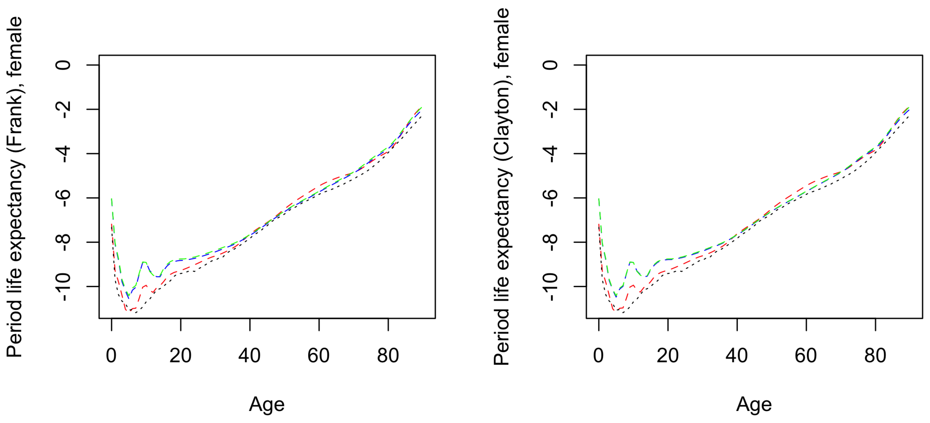
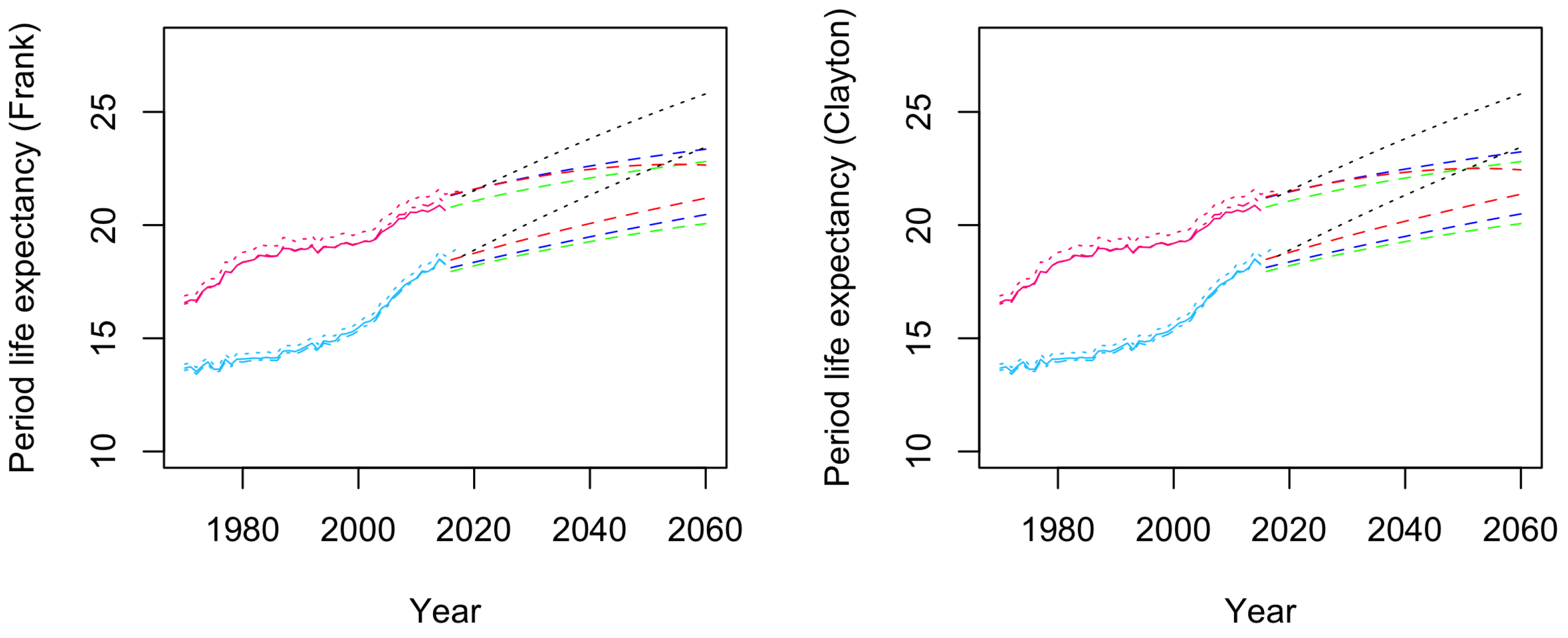
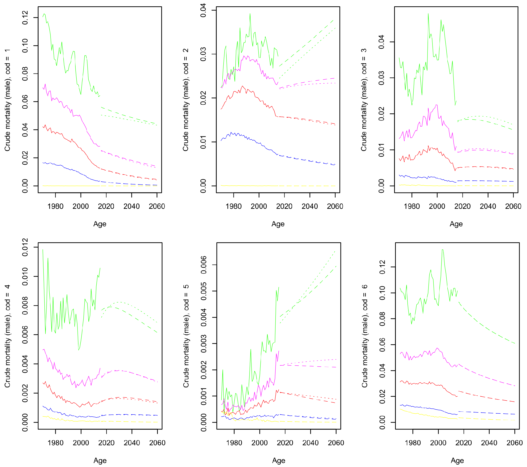
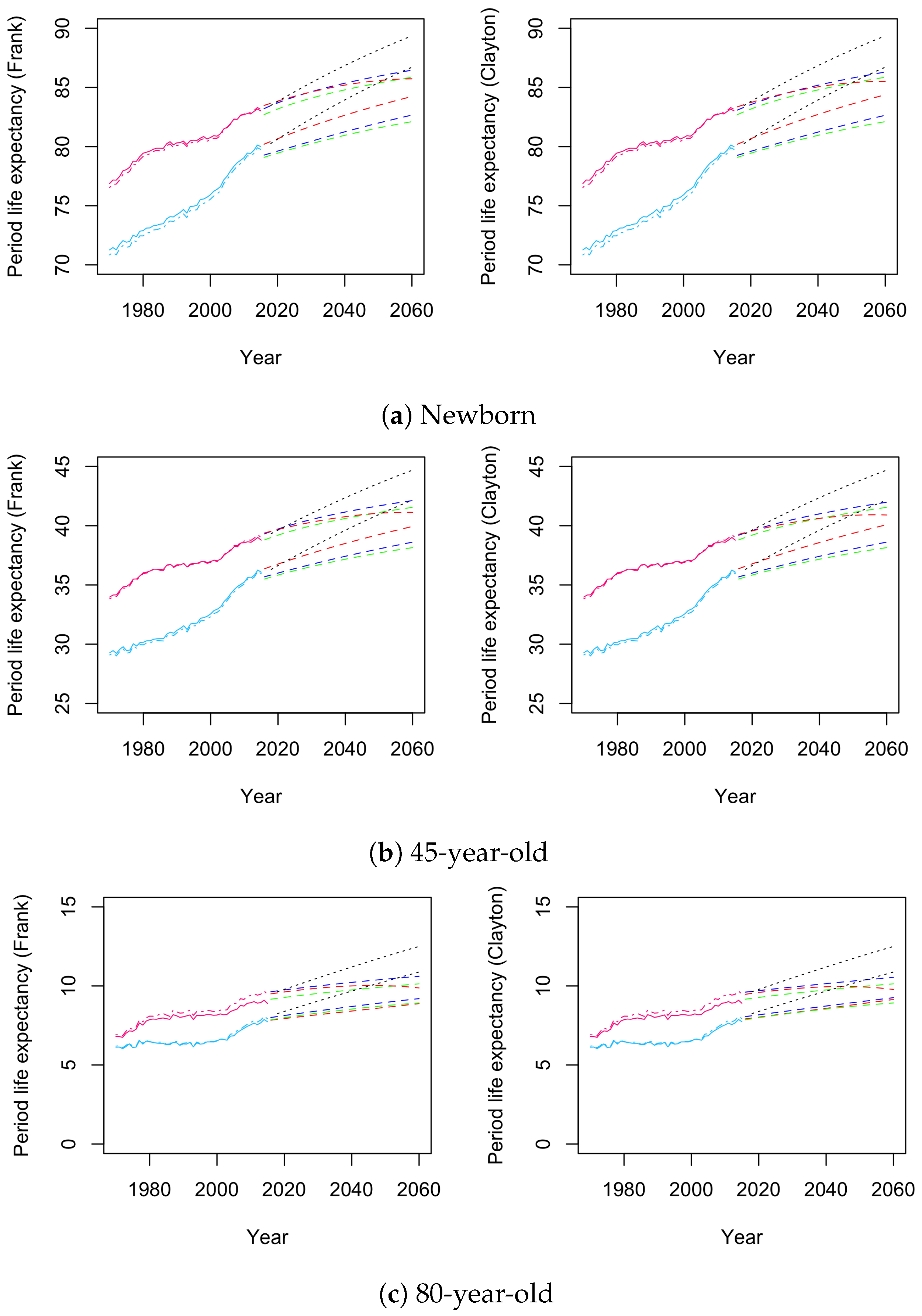
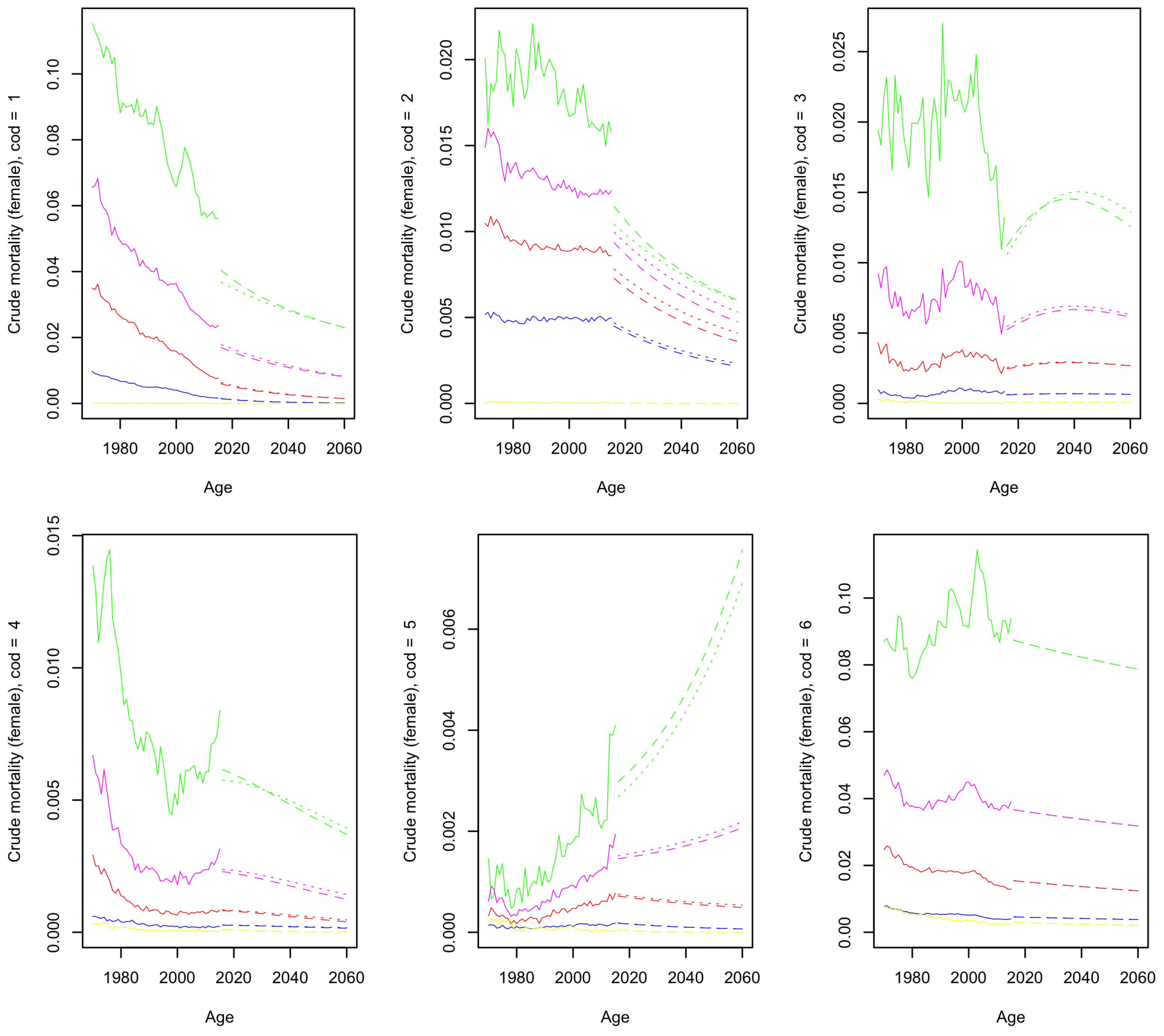
4. Numerical Results

We firstly present the estimation results for the crude and net mortality to then assess the forecasting performance and how it translates into population dynamics. Based on Li and Lu (2019), this was performed under the assumption of both a Clayton and Frank survivor copula with the parameter θ = 2 .16

4.1. Estimation

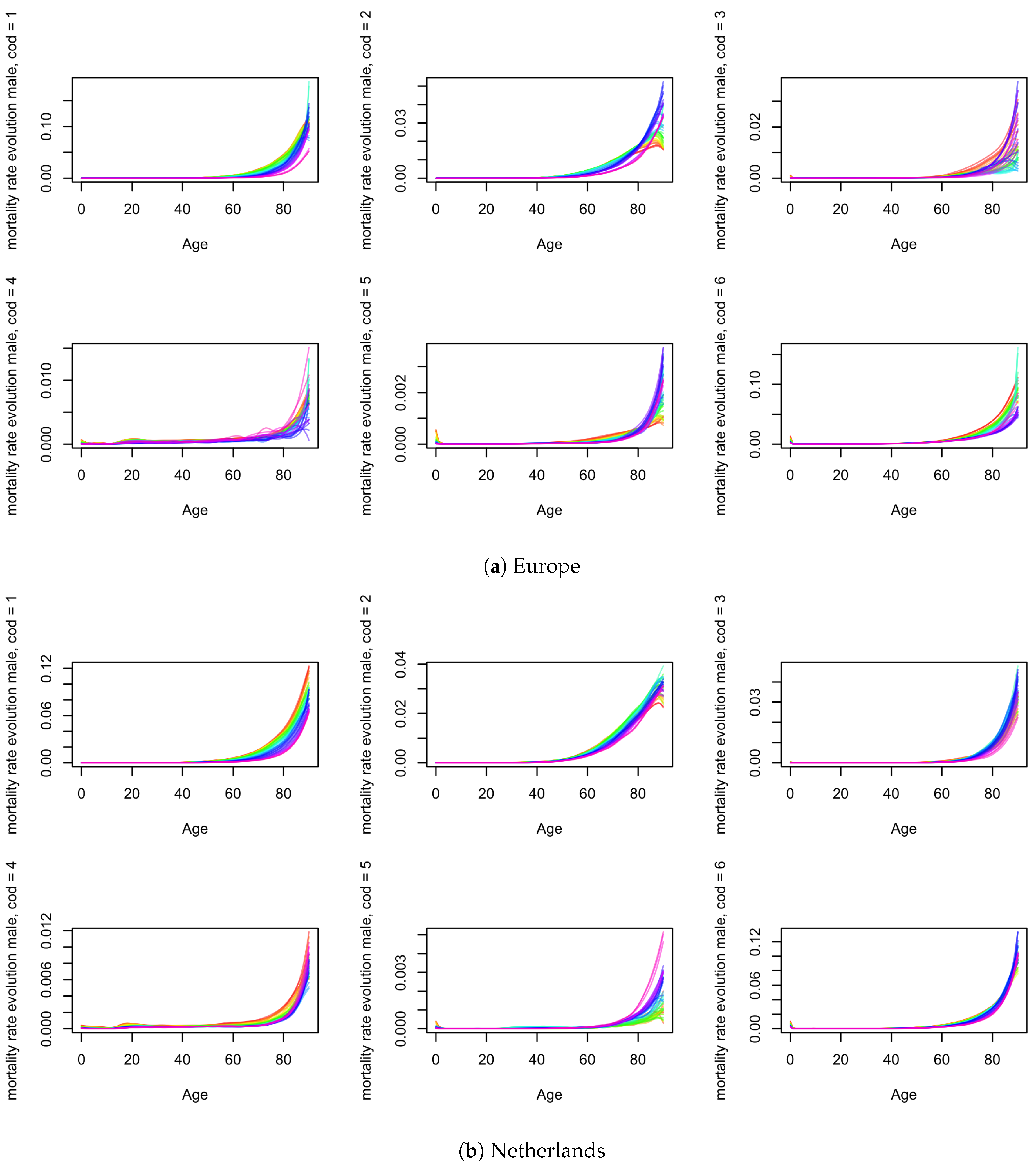
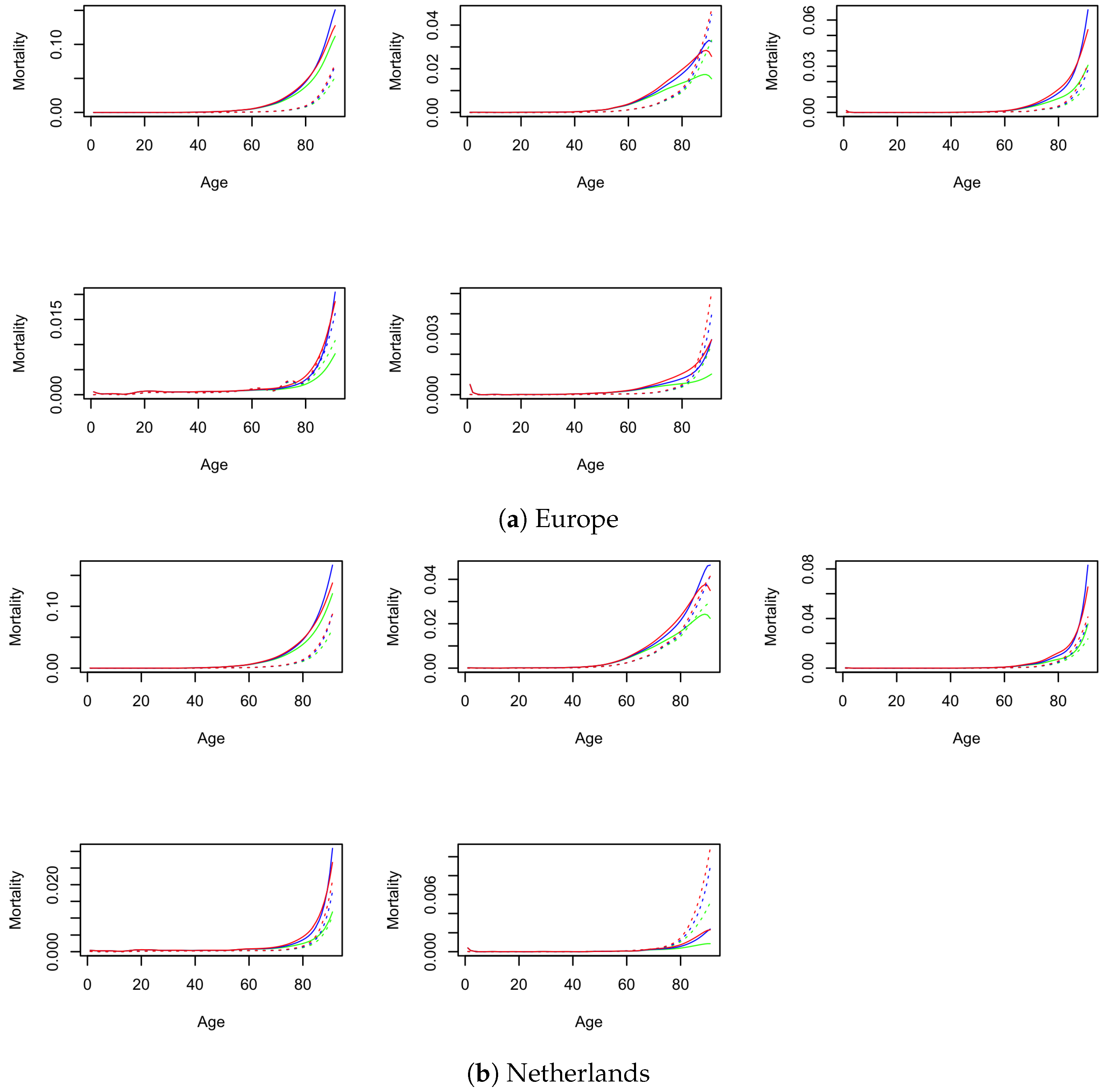
4.1.1. Crude Mortality

We applied Equation (2) and obtained the crude mortality for the EU and NL data depicted in Figure 3a,b, respectively, for females and Figure A1a,b in Appendix C for males. The year 1970 is represented by the red line and the last year, i.e., 2015, is drawn in violet. The years in between are represented by a rainbow colour ramp between these two colours. Firstly, in general, male mortality is higher than female mortality. We observe the biggest portion of mortality comprised by circulatory causes (cod 1). Male mortality exceeds that of females for circulatory, cancerous and respiratory diseases (cod 1, cod 2 and cod 3). Especially for cancer, mortality levels are double and for some ages/years even triple. In total, it can be concluded that most deaths fall under the categories of circulatory diseases and other causes. We then see that cancer has the second highest mortality rate. For newborns, mortality is mostly comprised of death caused by infectious diseases or external/other causes (cod 4, cod 5 and cod 6). We also observe a much higher mortality rate for males due to external causes (cod 4) around adolescent ages, which is a known phenomenon commonly referred to as the ‘accident hump’.
Overall, we see a decline in mortality. For circulatory diseases (cod 1), we see the same trend, similar for both males and females. For cancer (cod 2), we observe an overall decline as well. In the EU, for males over 75 years old, the mortality rate rose, but has fallen again over the past decade. For females, cancer mortality has been stable over the years only to experience an abrupt shock recently. After this shift, it has again remained relatively stable. For the NL, cancer mortality decreases for females in contrast to the stable male mortality rate. The mortality trends of respiratory diseases (cod 3) are similar between males and females in both data sets. Mortality decreased in the first half of the data set for both, but increased almost back to the starting level afterwards. The only slight variation is for the male age group 55–80, for which the probability of death increased less than it did for females of the same age. Deaths from external causes (cod 4) have developed similarly for males and females. Overall trends for this cause imply that mortality increases after a period of decrease. For females, we observe a mortality increase from infectious or parasitic diseases (cod 5). Only for newborns had the mortality intensity decreased. The same happened for males, with the exception of the age group above 75, which has experienced a large mortality increase. Lastly, we see a general decrease in deaths under the category of other causes (cod 6).

4.1.2. Net Mortality

Following the transformation of the marginal survival function described in Equation (16), we obtain the marginal mortality intensities. For both EU and NL as well as for males and females, we present the results in Figure 4 and Figure A2 in Appendix C. We exclude the results for other causes (cod 6), as this category is assumed to be independent and therefore its net mortality matches its crude mortality.
When we compare the marginal mortality rates to the crude mortality rates, we observe that the marginal mortality exceeds crude mortality in all cases. This is in line with our expectations. The empirical data consisting of exposure- and cause-specific deaths is directly translated in the crude mortality. When death occurs from some cause, the individual implicitly cannot die from another. We can regard this mutual exclusion as the censoring of the real underlying stochastic process. In the literature, this is referred to as frailty (Marshall and Olkin 1988; Oakes 1989). Frailty implies that a hypothetical individual who has died during a certain time period from one of the competing risks is on average more vulnerable than an observed individual who has not died from any cause of death during the same period of time (Li and Lu 2019). The new theoretical mortality rates are attained by taking into account this effect. The copula captures the dependence of the marginal distributions within the joint distribution and can therefore be used to obtain the underlying latent variables: the net mortality intensities. Since we eliminated the ‘distortion’, we obtained mortality rates that exceed the crude mortality rates. Only in the case of cod 1 net mortality for males and females can we observe net mortality rates that approach the corresponding crude mortality (both EU and NL). This can be explained by the fact that this cause (circulatory diseases) is the main cause of mortality and is therefore less sensitive to the distortion of other causes.
For older ages, we see that the relative differences between crude and net mortality increase. This can be contributed to the fact that mortality is higher for these ages. The potential censoring probabilities become bigger for this reason and therefore the net and crude rates increasingly diverge.
The trends of the net mortality under the Frank copula assumption matches the Clayton model mortality trends almost one to one. We observe that for males in the earliest observations of both NL and EU, the Clayton mortality surpasses the Frank mortality for old ages. For females, we see the same property to a lesser degree. As time proceeds, the curves tend to run parallel. The Frank copula model yields higher mortality in general than the Clayton copula. Moreover, we observed that the increase in mortality starts with a bit of lag under the Clayton assumption compared to the Frank assumption.

4.2. Forecast Results

We attained the forecast time-dependent variable by assuming errors equal to zero. We then transformed the net mortality forecast to crude mortality using Equation (14). Graphical representations of these forecasts are given in Figure 5 and Figure A3 in the Appendix C. For illustrative purposes, we picked out a selection of ages to represent this section. These ages are 0, 70, 80, 85 and 90. These ages display high mortality rates, hence forecast trends are easy analysable.17 Moreover, we present the findings in a schematic overview in Table 2.
For males, we observe a forecast of crude mortality that is increasing for cod 2 and cod 5 for the ages above approximately 85. The ages below this threshold show a decreasing mortality trend. For all other causes we see a downward trend of mortality for all ages. In the case of cod 3 and cod 4, mortality slightly rises in the first phase of the forecast before continuing on a downward trend. Overall, we see plausible forecasts as the trends from the performed forecast continue the trends of the historical crude mortality of the NL data set. For cod 2, we do see a notable decline in the mortality level with respect to historical values, especially for the Clayton model. This can be explained by the effect of the common factor expression in the model, since mortality for the EU has been lower than that of the NL in the past—although only slightly.
Furthermore, for females, we see an increasing mortality for infectious and parasitic diseases (cod 5). In this case, this is true for all ages, but the effect is more significant for older ages. In contrast to their male counterparts, we see a decrease in mortality from cancer (cod 2). All remaining cause-specific mortality is predicted to decrease in the future as well. For causes 1 to 3 (circulatory diseases, cancer and respiratory diseases), we observe a shift in the mortality predictions compared to the historical data. In particular, cancer mortality is expected to be much lower than in the past for NL. Again, this can be contributed to common factor specification, as EU mortality is lower than that of the NL for these causes. In particular, we want to highlight the shock decrease in cancer (cod 2) mortality for the EU around a decade ago from 0.010 to 0.005 while Dutch cancer mortality for females steadily decreased from 0.020 to 0.015. This large difference in EU and NL cancer (cod 2) mortality is translated by the common factor in the NL mortality forecast for females. The shift for age 90 circulatory diseases (cod 1) has the same explanation. The other ages did not experience a comparable shock. This is true since the difference between EU and NL mortality does not hold for all age groups, which is the case for cancer. The increase in cod 2 and 5 for males and cod 5 for females follows from the data as discussed in Section 4.1.1 and model specification. Indeed, Figure 3 and Figure A1 indicate such an evolution in older ages. A possible interpretation could be that vascular disease and cancer are positively correlated and the most recent innovations have helped reduce cardiovascular disease and lower the mortality of that cause. Hence, individuals have become less likely to die of vascular disease and more likely to die from cancer (Lyu et al. 2020).
We will subsequently compare the forecasts under the Frank copula assumption and the Clayton assumption. Since other causes (cod 6) are considered as independent censoring, the net mortality forecasts for both the Frank and Clayton model match the crude mortality forecast.
Due to the different dependence structure of the two copulas, we see alternative outcomes from the mortality forecasts between the models. For males, we can see that the mortality forecast from the Clayton model generally lies above that resulting from the Frank model. For circulatory diseases (cod 1), the dissimilarity is not very distinct. Moreover, for circulatory and parasitic/infectious diseases (cod 2 and 5) we observe that the expected mortality according to the Frank model exceeds that of the Clayton model for age 90. For females, we see a general exceedance of the Frank model for cod 1 and 2 (circulatory diseases and cancer). For cod 5 and cod 3 (parasitic/infectious diseases and respiratory diseases), the opposite is true. We confirm the same claim to be true for cod 5 (parasitic/infectious diseases), with the exception of age 90.
In order to be able to compare our model with the recent empirical case study by Li et al. (2019), we present the logarithm of mortality per age in 2050 of our forecast. Their results are based on male cause-specific US mortality and are estimated using a single-population LC model. Figure 6 and Figure A4 in Appendix C show the logarithm of mortality from age 0 to 90 in 2050 for multiple models. Firstly, the prognosis from Antonio et al. (2017) and our model (using θ = 2 ) are presented. Second, the independence model (i.e., our model using θ = 0 ) was included. This model is equivalent to a multi-population cause-specific mortality model applied to crude mortality instead of net mortality and can be regarded as similar to the one developed by Lyu et al. (2020). Finally, the single population (Lee–Carter) cause-of-death model is added. This model incorporates cause dependence using Archimedean copulae ( θ = 2 ) and is similar to the model by Li and Lu (2019).
We observe that, in most cases, the forecast for 2050 as obtained from our model is more pessimistic than its single-population counterpart. In the case of females between 40 and 65, we see that mortality in our model is lower. Furthermore, we see that the forecasts from our model behave less erratically than the single-population model. We derive this from the distance between the log-mortality of both models with respect to the Antonio et al. (2017) model. We see that the distance between the lines deviates more for the single-population model in comparison with our common factor model. This observation could indicate the stronger susceptibility of the single population model to the incidental deviation of Dutch cause-specific mortality with respect to our common factor model. All of the statements mentioned earlier in this paragraph hold for the Frank as well as the Clayton model specification.
From the graphs, we can conclude that all three cause-specific mortality models forecast lower future mortality. This observation is consistent with Li et al. (2019); Wilmoth (1995). Their papers describe how combining separate cause-specific mortality forecasts leads to lower mortality projections than the projections directly generated from aggregate mortality. The rationale behind this is that by using total aggregate mortality, the model loses information from cause-of-death mortality intensities. From the outcomes in the illustrations, we also conclude that the independence model is less optimistic than our model. This is also described in Li et al. (2019) and can be attributed to the dependence structure of the different causes of death.

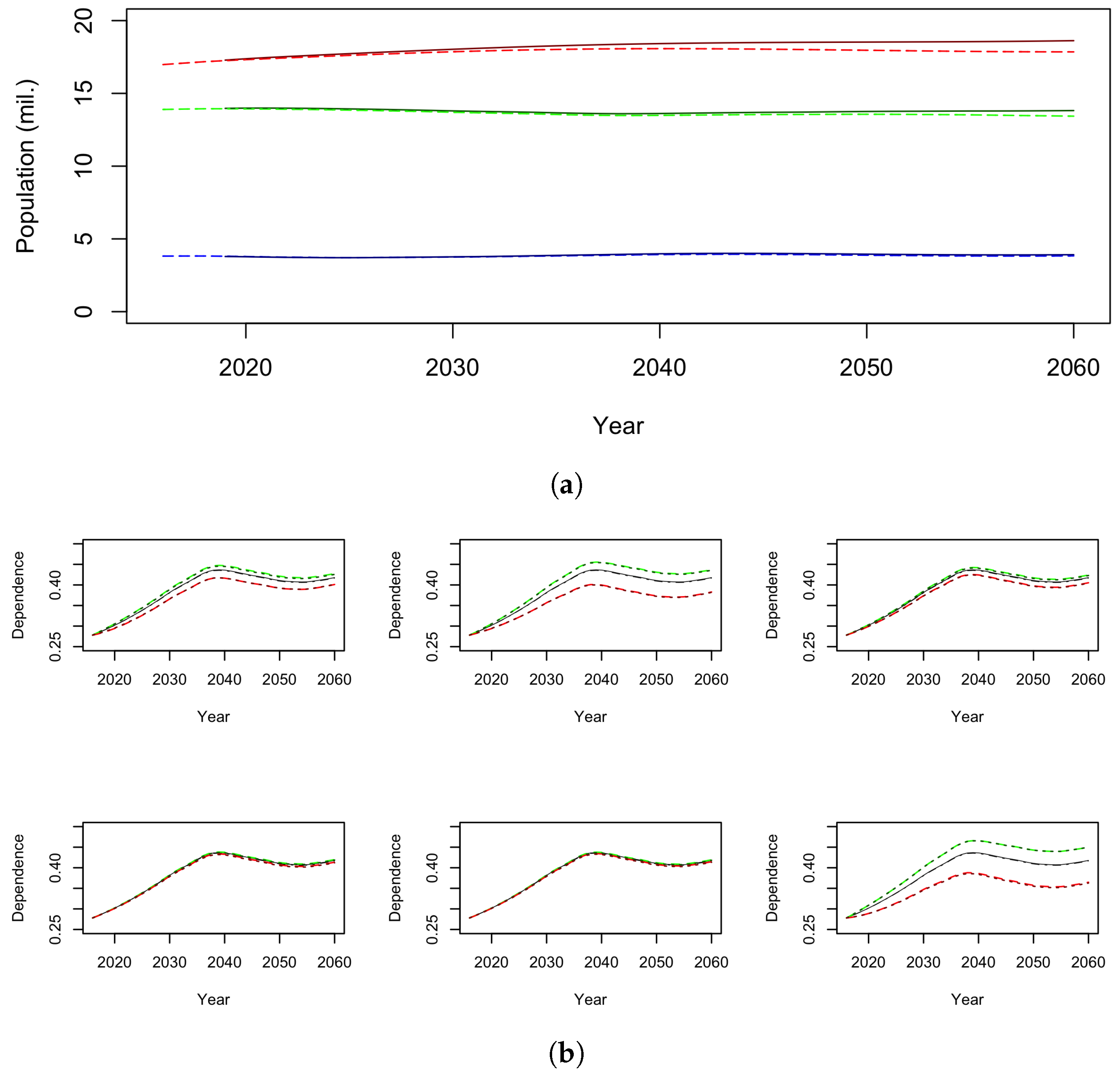
4.3. Population Dynamics

In Figure 7a, we illustrated the expected evolution of the age groups 0–20, 0–65 and all ages. This forecast was performed for the years 2016 and 2060 and for a model with the dependence coefficient θ equal to 2 based on Li and Lu (2019). We expect the fraction of the Dutch population younger than 20 to remain relatively steady over the upcoming years. The number of people between the ages of 20 and 65 will decrease between 2016 and 2040. After this period, this trend will reverse and the age group will increase in size for the remainder of years. The biggest change in population composition will be ascribed to the old age group, namely people above 65 years old. More people belonging to the generation of baby boomers will pass the threshold of 65 years old in the upcoming years and therefore the fraction of people of old age will increase across the population. The same observation has been put forward by Boumezoued et al. (2018), although for the French population. Despite the observed similarities, when we compare our model forecast to that from CBS, we see a slight deviation between both predictions. We assume that this results from the excess mortality inherent to our NL data set.
Furthermore, we included a comparison of future dependency ratio expectations for hypothetical cases of reduction and increase in marginal mortality for all six causes. This comparison is shown in Figure 7b. The theoretical cases are that of halving and doubling the net mortality. Again, the shown results are under an assumed dependence coefficient equal to 2. The dependency ratio will grow between 2016 and approximately 2040. After this maximum, it dips down after which it starts to increase again. We see that an increase in net mortality of factor 2 yields a larger absolute change in dependency ratio than that induced by a modification of factor 0.5. Furthermore, we observe no significant difference between the results under the assumption of a Frank or Clayton survivor copula.18 In addition, we conclude from the graphs that the sensitivity of the dependency ratio to net mortality shocks was the largest for cod 6, which is in line with expectations. Since the variable is considered as independent censoring, an increase/decrease in its mortality risk will not coincide with a decrease/increase in the other causes through the frailty principle.
Surprisingly, we see that the second largest sensitivity is observed for cancer (cod 2). Since we alter net mortality by the multiplication of a factor, it would be sensible to observe the largest sensitivity for the cause of death with the largest mortality contribution, in our case, cod 1 (circulatory diseases). From this, we can deduce that cod 1 suffers from a larger dependence between other causes than cod 2, hence the muzzled impact of the applied disturbance. The rationale behind this could be as follows. It seems reasonable to assume that for a hypothetical individual, a relatively high cod 1 mortality risk often coincides with an unhealthy life style. This is possibly even more the case than for cancer. This would indeed implicate a higher frailty of such a particular individual and therefore a stronger dependence with other causes. Boumezoued et al. (2018) predicted a comparable increase in future dependency in the case of either the removal of circulatory diseases (cod 1) or the removal of cancer (cod 2). This contradicts our findings. This alternative conclusion can be ascribed to their choice of independent cause-specific mortality and therefore the lack of frailty incorporated into their model. This is backed up by our findings on dependence sensitivity for other causes (cod 6), which similarly to the model from Boumezoued et al. (2018), is assumed to be independent. We can see that their findings for the removal of this specific cause in their research are comparable to ours.

4.3.1. Model Outcomes

To validate our model, we present measures under Frank and Clayton copula specification for different values of the copula dependence coefficient θ { 0.5 , 1 , 2 , 5 } as well as for the independence copula case θ = 0 which allows us to compare it to an LL model for the cause-specific crude mortality. Furthermore, we will show the levels for different shocks of cod 3 (respiratory diseases).
Independence copula and general effects
As shown in Table 3 (and Table A1 in Appendix D), under the assumption of an independence copula and without the presence of any shocks, the dependency ratio grows with 10.5% points from 29.2% in 2020 to 39.7% in 2040. In the following years, the dependency ratio decreases with 2.1% points to 37.6% in 2060. Respectively, for r = 0.5 or r = 2 , these differences become 11.0% and 2.0%, or 9.5% and 2.2%.
Furthermore, under the independent copula specification, we observe a growth of period life expectancy for males of 1.86 ( r = 1 , from 18.21 to 20.07), 1.95 ( r = 0.5 , from 18.51 to 20.46) and 1.71 ( r = 2 , from 17.64 to 19.35). For females, these values are 1.74 (from 21.07 to 22.81), 1.83 (from 21.32 to 23.15) and 1.59 (from 20.59 to 22.18). The conclusion we are able to draw from this result is that the life expectancy increase is enhanced in the case of halving the net respiratory mortality. The opposite is the case for the doubling of marginal mortality for this category. This finding is directly connected with our findings for future population dependency. We observed that the absolute change in the dependency ratio was bigger for a reduction in net mortality. This is explained by the fact that the rate of increase is also affected by net mortality modification. From the outcomes, we derive that in the independence copula case, the male period life expectancy increases at a higher rate than that of female life expectancy. This is even more strongly the case for any model composition included. This is in agreement with the conclusions drawn from the Antonio et al. (2017) projections.
Cohort life expectancy in 2020 for males equals 18.83 ( r = 1 ), 19.19 ( r = 0.5 ) and 18.18 ( r = 2 ). For females, the corresponding levels are 21.70, 22.02 and 21.11. In direct relation to the similar findings for period life expectancy, the higher absolute difference for r = 2 with respect to r = 1 than r = 0.5 confirms the stronger effect of doubling net mortality compared to halving net mortality. For both sexes, the cohort life expectancy values produced by our model when no shock is experienced are lower with respect to those calculated by Antonio et al. (2017). The cohort life expectancy for a 65-year-old male equals 20.3 in 2018. For females, this value equals 23.1. The cohort life expectancy is higher than the period life expectancy in 2020 for both sexes. This holds for all selected model specifications. From this conclusion, we can deduce that the overall mortality rates decrease in the future, regardless of the model selected.
Respiratory disease shocks
As expected, when net mortality for respiratory diseases halves, we generally see an increase in the future dependency ratio for all years and we confirm that the opposite effect occurs for a doubling of net mortality. In 2060, these upward and downward shifts amount to 0.8% and 1.6% for the independence copula, respectively. In general (i.e., for all θ and both the Frank and Clayton assumptions), we observe a dependency ratio after a factor 2 shock of net cod 3 mortality (respiratory diseases) that is higher than that in the case of no shock. Similarly, the net mortality for no shock exceeds that in the case of a halving of net mortality. Directly corresponding, we also see these effects for period life expectancy and cohort life expectancy for all models. These findings are in line with intuition.
We now consider the direct effect of the net mortality shocks on the presented measures. We again observe that a doubled net mortality has more impact on the mortality measures than the halving of net mortality. This finding holds for all models and agrees with the earlier conclusions drawn from Figure 7b.
Dependence
We then turn to the differences ( Δ ) in Table 3. These coefficients compare all measures with respect to their corresponding counterparts which are presented for the independence model. The findings that we will first devote our attention to are the different effects of an increase in the dependence coefficient for the Frank and Clayton models. We see for all measures that when θ is increased under Frank specification, their relative difference to their corresponding measure under assumed independence becomes bigger. This can be observed by increasing values for Δ for the Frank model as we move down in the table (i.e., increasing the assumed θ ). Hence, when strong dependence between causes is assumed, crude mortality is expected to decrease more quickly with respect to independent causes then when lower dependence is assumed. For instance, when θ = 0.5 and r = 2 is assumed, the difference with the independent model in terms of dependency ratio in 2060 is negligible ( Δ = 0.0 % ). When we increase the assumed dependence coefficient to a level of 5, this difference becomes 2.6%. Conversely, this holds for the Clayton model. In the Clayton environment, we see that the differences decrease as θ increases. This effect is seen in the individual mortality model of Li and Lu (2019) for a change of θ = 0.2 to θ = 1 . Afterwards, the effects for the Clayton model are the same as for the Frank model when θ is increased. We derive that this effect is therefore the result of the common factor formulation of our model. Furthermore, we can see that in the case of θ = 2 , the Frank and Clayton outcomes are comparable. When we look back at Figure 7b, we see that for all shocks and for all causes, the outcomes for the dependency ratio measure are similar for the Frank and Clayton models and thus that this model property for θ = 2 holds across causes.
Finally, we determine that the inclusion of dependence between the various causes of death makes the mortality decrease in a general fashion. This can be observed by the strictly positive deltas. This can be explained by means of the frailty principle. We therefore conclude that the reduction in mortality from a cause in the forecast is never fully replaced by that of other causes. On the contrary, an increase in mortality does not lead to a bigger or equivalent decrease in mortality of other causes. This is a logical determination. We do see that this effect in some cases decreases. In those cases, the delta in 2020 exceeds that of 2060.

4.3.2. Model Comparison

We now turn our attention to Figure 8. We have presented in the illustration the period life expectancy prognoses for 65 year olds that result from different models. We present the expectancies for three different models using our constructed data.
We study our model with θ = 2 , θ = 0 as in Lyu et al. (2020)19 and the Lee–Carter specified cause-specific model with the Archimedean copula with θ = 2 as in Li and Lu (2019). Moreover, we included the overall mortality model prognosis from Antonio et al. (2017) as a baseline model to compare the cause-specific mortality models with. In order to create a frame of reference, we included in the graph the observed historical period life expectancy. Again, we observe the slight underestimation of the actual mortality in our data set.
When we compare the cause-specific prognoses with the forecast from Antonio et al. (2017), we see that all models expect a much lower decrease in mortality in the following decades. This is depicted by the smaller increase in the life expectancy of people aged 65. This is in line with the conclusion drawn from Figure 6 and Figure A4. The most notable and remarkable is that between the independence copula and the Antonio et al. (2017) baseline model. We see that if we forecast crude cause-specific mortality individually in a common factor context, the estimated prognosis is much lower than that in a non-cause-specific environment. The difference in period life expectancy amounts to more than 3 years in 2060.
The variation between the prognosis results sheds light on the difference between forecasting overall mortality versus forecasting mortality per cause of death. We see that forecasting each cause individually instead as a whole has drastic consequences for the expected future mortality intensities. Since the line depicting the single population mortality forecast lies much lower than the forecast based on general mortality, we should ask the general question of whether using cause-specific mortality is the right way to forecast future population-wide mortality. Vice versa, it shows that the constant reassessment of the currently used mortality model is a serious necessity since we have seen that different forecasting methods yield very different outcomes.
We determined earlier that the forecast of the model using θ = 2 exceeds that of the independence copula model. Moreover, this surplus increases as the forecast horizon increases. Furthermore, significant differences can be observed between our model and the cause-specific mortality model without the common factor addition. We see that in the latter model, the strong convergence of the prognoses of males and females occur. For females, we see in historical data that mortality has decreasingly increased since 2005. For the most recent years, the mortality decrease for females has almost stalled and even decreased in some years. Due to the stronger susceptibility to the incidental deviation of the model without a common factor element, it is possible that this short-term trend, which is likely to be incidental, is translated into the forecast with more weight than that compared to the common factor model. This could result in questionable forecasts, which is the case for females in this model. Our model in turn shows more resistance to the short-term effects within Dutch mortality with the incorporation of the common factor. This proves increased robustness for our forecasting model with respect to a single population model. We see that the aforementioned conclusions hold for multiple ages as shown in Figure A5a–c in Appendix D.

5. Conclusions

In this research, we discuss an extension to the frequently applied Antonio et al. (2017) mortality model. This model offers a way to model cause-specific mortality for the Netherlands, whereas the original model solely focusses on overall mortality. The estimation of the model is based on Dutch cause-of-death data from CBS and data for 14 comparable European countries retrieved from the WHO Mortality Database. We incorporated an Archimedean copula dependence structure to capture the dependence between cause-specific mortality for five different cause of death categories. This method has been previously discussed in a single population context by Li and Lu (2019). This is the first time the prominently used mortality model from Antonio et al. (2017) has been extended in such exhaustive manner for cause-specific mortality.
The model was used to simulate future Dutch population dynamics based on the cause-specific mortality forecast and demographical influx forecasts from CBS. We conclude that, in general, cause-specific mortality models forecast a much higher/lower expected future mortality/life expectancy with respect to general mortality models. The difference in period life expectancy can amount to more than 3 years in 2060. This encourages deeper research into this topic, since the differences and hence the possible implications are significant. Moreover, we find that the inclusion of the common factor in the cause-specific mortality context leads to more robust mortality forecasts, less sensitive to the incidental deviation of observed cause-specific mortality, in comparison to the single population counterpart.
We would like to highlight a few points of interest. We recall that a great amount of information on cause-specific mortality for the EU is absent for ICD-10. In order to counter this, we used comparability ratios, which in turn lead to more volatile data. Obviously, this is a possible point of improvement. Furthermore, please note that we solely considered the model uncertainty of the model. We did not treat the parameter uncertainty of the parameters. We suggest that this could be performed in further research on this topic. Using the Poisson distribution of the net mortality rates to bootstrap artificial data sets and in turn estimate the corresponding parameters, the differences between the parameters can then be analysed.

Supplementary Materials

The following are available online at https://www.mdpi.com/article/10.3390/risks9120221/s1, Table S1: Final year of implementation of the ICD codes per country for the total cause-specific data set 1970–2015, Table S2: Cause-of-death coding of the different classification systems, Figure S1: The effect of the comparability transformation, Figure S2: The effect of the comparability transformation, Figure S3: The effect of the comparability transformation, Figure S4: The effect of the comparability transformation, Table S3: Details of manipulated instances for insufficient data, Figure S5: Cause-specific mortality intensities of the 14 selected countries in the data set after coping with the inherent data difficulties (1970–2015), Table S4: WHO Mortality Database formatting, Figure S6: Age-specific constant for Frank (solid line) and Clayton (dotted line) models (EU), Figure S7: Age-specific constant for Frank (solid line) and Clayton (dotted line) models (NL), Figure S8: Age-specific trend sensitivity for Frank (solid line) and Clayton (dotted line) models (EU), Figure S9: Age-specific trend sensitivity for Frank (solid line) and Clayton (dotted line) models (NL), Figure S10: Time trend for Frank (solid line) and Clayton (dotted line) models (EU), Figure S11: Time trend for Frank (solid line) and Clayton (dotted line) models (NL), Table S5: Estimated coefficients of the SUR reestimation of the estimated time dependent variables K c = { K ^ e u c , M ( t ) , k ^ n l c , M ( t ) , K ^ e u c , F ( t ) , k ^ n l c , F ( t ) } , Figure S12: Crude mortality forecast for the Netherlands based on our cause-specific mortality model ( θ = 2 ), male (Frank), Figure S13: Crude mortality forecast for the Netherlands based on our cause-specific mortality model ( θ = 2 ), female (Frank), Figure S14: Crude mortality forecast for the Netherlands based on our cause-specific mortality model ( θ = 2 ), male (Clayton), Figure S15: Crude mortality forecast for the Netherlands based on our cause-specific mortality model ( θ = 2 ), female (Clayton).

Author Contributions

Conceptualization, J.A.-G.; Formal analysis, G.Z.; Methodology, J.A.-G.; Supervision, J.A.-G.; Visualization, G.Z.; Writing—original draft, G.Z.; Writing—review and editing, J.A.-G. All authors have read and agreed to the published version of the manuscript.

Funding

This research received no external funding.

Data Availability Statement

Data used in this paper is available at https://statline.cbs.nl/Statweb/ (accessed on 28 February 2019) and https://www.who.int/healthinfo/statistics/mortality_rawdata/en/ (accessed on 28 February 2019).

Conflicts of Interest

The authors declare no conflict of interest.

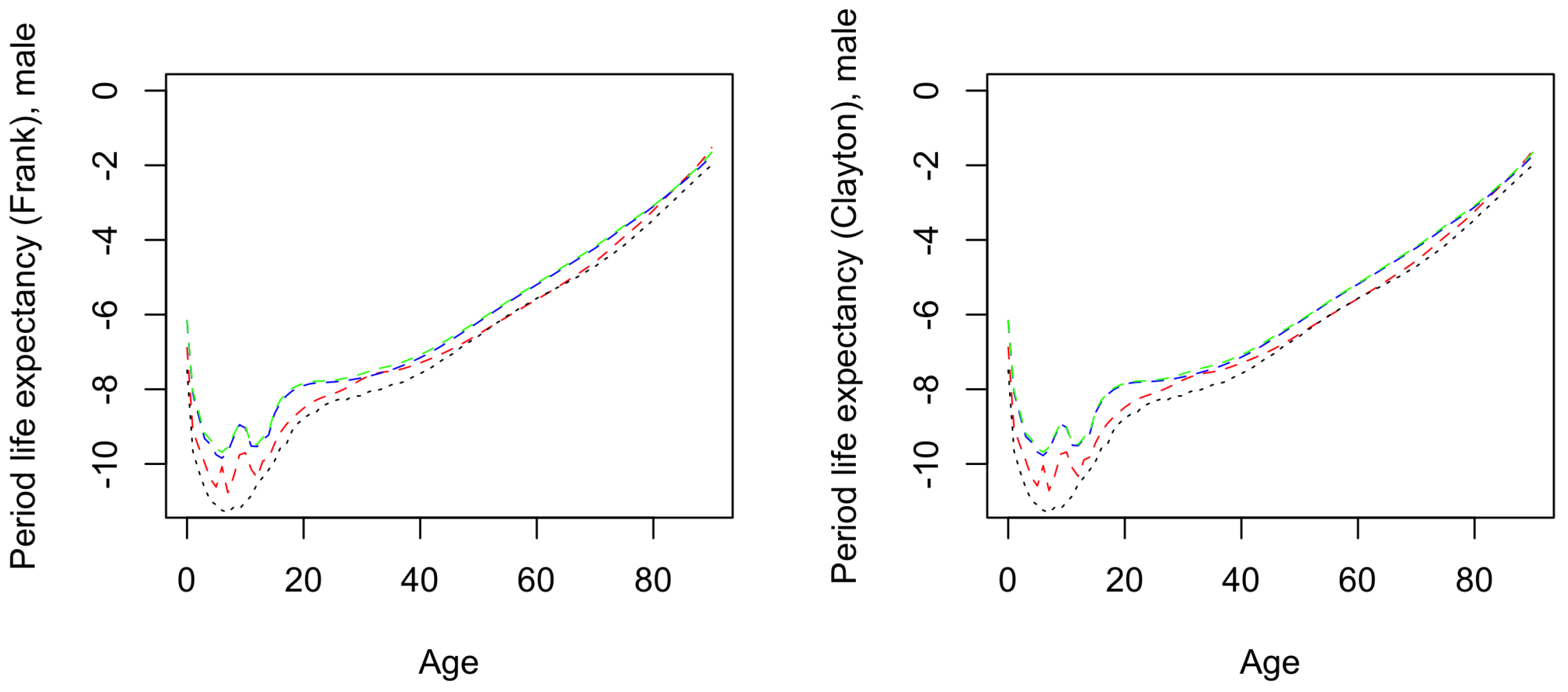
Appendix A. Frank and Clayton Copula Definition and Generator Function

In the equation below, we present the definition of the Frank and Clayton copula and the corresponding inverse and first order derivative of their generator function ψ ( t ) . For all u 1 , , u z [ 0 , 1 ] :
Frank : S ( S ( u 1 ) , , S ( u z ) ) = 1 θ ln [ 1 + ( e θ u 1 1 ) . . . ( e θ u z 1 ) ( e θ 1 ) m 1 ] ,
ψ ( t ) = e θ 1 θ ( e t + θ + 1 e θ ) ,
ψ 1 ( t ) = ln e θ t 1 e θ 1 .
Clayton : S ( S ( u 1 ) , , S ( u z ) ) = u 1 θ + + u z θ z + 1 1 θ ,
ψ ( t ) = θ ( 1 + t ) θ 1 ,
ψ 1 ( t ) = t 1 θ 1
The reverse formulation of equation of (13) is derived in the following way. For x 0 :
S i c ( x , t ) = ψ s = 0 x exp u = 0 s k = 1 z * m i k ( u , t ) ψ ψ 1 exp u = 0 s k = 1 z * m i k ( u , t ) · m i c ( s , t ) , ψ 1 S i c ( x , t ) = s = 0 x S i ( s , t ) ψ ψ 1 S i ( s , t ) · m i c ( s , t ) , S i ( x , t ) ψ ψ 1 S i ( x , t ) · m i c ( x , t ) = s = 1 x 1 S i ( s , t ) ψ ψ 1 S i ( s , t ) · m i c ( s , t ) ψ 1 S i c ( x , t ) , m i c ( x , t ) = ψ 1 ( S i c ( x , t ) ) s = 1 x 1 S i ( s , t ) ψ ψ 1 S i ( s , t ) · m i c ( s , t ) S i ( x , t ) ψ ψ 1 S i ( x , t ) ,
for x = 0 , we obtain:
m i c ( 0 , t ) = ψ 1 ( S i c ( 0 , t ) ) S i ( 0 , t ) ψ ψ 1 S i ( 0 , t ) .

Appendix B. Maximum Likelihood Estimation of (24)

Step 1:
We return to the Li–Lee formulation. First, we focus on the common factor expression described in Equation (20) for which MLE is to be performed. In our case, this is represented by the data for EU. The restriction imposed by this equation and the substitution of m i C F ( x , t ) by λ e u c ( x , t ) leads to the following equation:
λ e u c ( x , t ) = e A e u c ( x ) + B e u c ( x ) K e u c ( t ) .
Inserting (A8) into the log-likelihood equation from (24) yields:
e u c ( x , t ) = x t [ D e u c ( x , t ) · ln { E e u ( x , t ) · e A e u c ( x ) + B e u c ( x ) K e u c ( t ) } E e u ( x , t ) · e A e u c ( x ) + B e u c ( x ) K e u c ( t ) ln { D e u c ( x , t ) ! } ] = x t [ D e u c ( x , t ) · ( ln { E e u ( x , t ) } + A e u c ( x ) + B e u c ( x ) K e u c ( t ) ) E e u ( x , t ) · e A e u c ( x ) + B e u c ( x ) K e u c ( t ) ln { D e u c ( x , t ) ! } ] .
The parameter estimates A ^ e u c ( x ) , B ^ e u c ( x ) and K ^ e u c ( t ) are found by maximising the log-likelihood function in Equation (A9). For this, we use the Newton–Raphson method (Newton 1833; Raphson 1702). For MLE, the restrictions from Equation (19) are applied, forcing the sum of K ^ e u c ( t ) and B ^ e u c ( x ) to be equal to 1 and 0, respectively.
Step 2:
Then, we turn to the unique tendencies of the individual population with respect to the common factor effect of the group and we state the restriction as in Equation (21) by inserting the optimal values for A e u c ( x ) , B e u c ( x ) and K e u c ( t ) found in the first step in the following manner:
λ n l c ( x , t ) = e A ^ e u c ( x ) + B ^ e u ( x ) K ^ e u c ( t ) + a n l c ( x ) + b n l c ( x ) k n l c ( t ) = λ ^ e u c ( x , t ) · e a n l c ( x ) + b n l c ( x ) k n l c ( t ) .
Comparable to step 1, we now plug in (A10) into Equation (24) and obtain the subsequent statement:
n l c ( x , t ) = x t [ D n l c ( x , t ) · ln { λ ^ e u c ( x , t ) E n l ( x , t ) · e a n l c ( x ) + b n l c ( x ) k n l c ( t ) } λ ^ e u c ( x , t ) E n l ( x , t ) · e a n l c ( x ) + b n l c ( x ) k n l c ( t ) ln { D n l c ( x , t ) ! } ] = x t [ D n l c ( x , t ) ( ln { λ ^ e u c ( x , t ) E n l ( x , t ) } + a n l c ( x ) + b n l c ( x ) k n l c ( t ) ) ) λ ^ e u c ( x , t ) E n l ( x , t ) · e a n l c ( x ) + b n l c ( x ) k n l c ( t ) ln { D n l c ( x , t ) ! } ] .
The Newton–Raphson method is used in order to attain the maximum of the log-likelihood function from (A11). Furthermore, following the guidelines set from (19), we set the sum of b n l ( x ) and k n l ( t ) equal to 1 and 0, respectively. As a result, we obtain the fitted estimates of the involved parameters, denoted as a ^ n l c ( x ) , b ^ n l c ( x ) and k ^ n l c ( t ) .

Appendix C. Crude and Net Mortality for Males

Figure A1. Crude male mortality per age from historical data, for causes of death 1–6. A rainbow colour ramp is used to represent the course of years from red (1970) to violet (2015).
Risks 09 00221 g0a1
Figure A2. Comparison of the NL and EU crude (green) and net male mortality intensities from the Frank (red) and Clayton (blue) model. The solid lines represent 1970 and the dotted lines represent 2015.
Risks 09 00221 g0a2
Figure A3. Crude male mortality forecasts compared (Frank = dashed, Clayton = dotted). Age: 0 = yellow, 70 = blue, 80 = red, 85 = magenta, 90 = green.
Risks 09 00221 g0a3
Figure A4. The male log-mortality in 2050 for ages 0–90. Included are: the comparative model from Antonio et al. (2017) (black), the independence model (green), the single population model (red) and our model (blue). θ = 2 is assumed.
Risks 09 00221 g0a4

Appendix D. Robustness Checks

Table A1. The resulting properties of forecasts using our cause-specific multi-population mortality model. Presented are the outcomes under different assumed dependence coefficients ( θ ) and respiratory disease shocks (r). The included coefficients are: the dependency ratios in 2020, 2040 and 2060 ( d 2020 , d 2040 , d 2060 ), the period life expectancy for males and females in 2020 and 2060 M l 2020 p , M l 2060 p , F l 2020 p , F l 2060 p ) and the male and female cohort life expectancy ( M l 2020 c , F l 2020 c ).
Copular d 2020 d 2040 d 2060 M l 2020 p M l 2060 p F l 2020 p F l 2060 p M l 2020 c F l 2020 c
Independence
-0.2920.3970.37618.2120.0721.0722.8118.8321.70
0.50.2940.4040.38418.5120.4621.3223.1519.1922.02
20.2880.3830.36117.6419.3520.5922.1818.1821.11
θ = 0.5
Frank-0.2920.3970.37718.2220.1521.2022.9218.8621.81
0.50.2940.4040.38518.5220.5321.4423.2519.2022.12
20.2880.3830.36317.6619.4620.7322.3118.2121.24
Clay-0.2950.4080.39518.6321.1623.0124.4919.4123.38
0.50.2960.4110.39718.7921.2123.0824.6019.5323.50
20.2920.4010.39118.1521.0122.8424.2519.0923.14
θ = 1
Frank-0.2920.3980.37918.2520.2521.3123.0518.8921.93
0.50.2940.4050.38618.5420.6121.5523.3519.2222.22
20.2890.3840.36517.7019.5820.8622.4618.2621.38
Clay-0.2940.4020.38518.4520.5721.9823.7519.1022.55
0.50.2950.4070.38918.6820.7822.1423.9719.3422.76
20.2910.3920.37517.9620.1621.6623.3318.6222.13
θ = 2
Frank-0.2930.4000.38318.3620.4621.5823.3619.0122.22
0.50.2950.4070.38918.6320.7721.7923.6319.3122.48
20.2900.3880.37017.8119.8521.1522.8218.4121.69
Clay-0.2930.4000.38318.3820.5021.4723.2319.0322.08
0.50.2950.4070.39018.6420.8121.6823.5119.3322.34
20.2900.3880.37117.8619.9021.0622.7118.4521.57
θ = 5
Frank-0.2980.4160.39919.1621.2522.5324.2719.7923.19
0.50.2990.4190.40219.3321.3522.6924.4219.9123.38
20.2950.4050.38918.5820.8122.0423.8619.2622.68
Clay-0.2930.3990.38018.3420.2821.2122.9718.9621.84
0.50.2950.4060.38718.6320.6421.4523.2919.2922.14
20.2900.3860.36617.8219.6120.7622.3918.3421.28
Figure A5. The observed period life expectancies for newborn, 45-year-old and 80-year-old males (blue) and females (pink) from our (solid) and the Antonio et al. (2017) (alternating) data set and the forecasts from Antonio et al. (2017) (black), the independence model (green), the single population model (red) and our model with θ = 2 (blue).
Risks 09 00221 g0a5

Notes

1
Source: Centraal Bureau voor de Statistiek.
2
For instance, the recent COVID-19 pandemic or an increase in the influenza virus-related deaths as observed by Actuarieel Genootschap (2018).
3
We refer to Enchev et al. (2017) for a survey and comparison of various multi-population models.
4
Enchev et al. (2017) analysed the ordinary Li–Lee model, two simplified versions of this model and the common age effect model of Kleinow (2015) and concluded that the regular Li–Lee model was the second-best performing model after the common age effect model.
5
Competing risks is the presence of censoring of the time of death from one cause in the event of death from another cause.
6
In addition to the clear extensions to the academic literature, we believe that the cause-specific extension is relevant for all practices which deal with longevity risk in the Netherlands and rely on the multi-population Antonio et al. (2017) model.
7
The LL model, as described in Antonio et al. (2017), is currently being used by Actuarieel Genootschap for the calculation of the Dutch life tables.
8
The idea of the copula, a multivariate distribution function with uniform marginal probability, was first presented in Sklar (1959). The method offers a way to examine the dependence of a joint distribution and its underlying marginal distributions of latent random variables.
9
The full definition of the survival functions as well as the first derivative and inverse of both corresponding generator functions are given in Appendix A, Equations (A1)–(A6).
10
Enchev et al. (2017) highlight the potential shortcomings in the re-estimation process of the time-dependent coefficient k i ( t ) . They suggest a vector autoregressive model of order 1 (VAR(1)) instead of the AR(1) proposed by Li and Lee (2005). This is due to the sometimes diverging properties of the AR(1) model in a multi-population context. By the use of the VAR(1) model and its underlying covariance matrix, coherent forecasting can be retained. Moreover, this forecasting method does not significantly deviate from individual AR(1) forecasts (Enchev et al. 2017).
11
We acknowledge that we use a reduced variable set. A more comprehensive model could study all population flows with their own distinct functions, as can be seen in, e.g., Boumezoued et al. (2018). However, this is beyond the scope of our paper.
12
https://statline.cbs.nl/Statweb/ (accessed on 28 February 2019).
13
14
https://statline.cbs.nl/Statweb/ (accessed on 28 February 2019).
15
Keeping in mind the slim volume of cause-of-death data in many cases, we chose to include mortality numbers from Germany between 1970 and 1989, when the current country of Germany was split into the Federal Republic of Germany (West Germany/FRG) and the German Democratic Republic (East Germany/GDR). This is in contrast to the general mortality data used by Antonio et al. (2017). Moreover, in previous cause-of-death research by Arnold and Sherris (2015), mortality data of split Germany were not included, since no data were available for the German Democratic Republic before 1969. This does not pose a problem in our research, because the first year of our data set is 1970, and therefore, we accumulated the mortality knowledge of the German subsections to represent the total German mortality for the years preceding the fall of the Berlin Wall.
16
The robustness of the parameter θ is analysed in Table 3 and Table A1.
17
For a full comprehensive display of the forecast, we refer to the illustrations in Figures S12–S15 of the Supplementary materials Section S.4.
18
This is not always the case, but results from our choice of dependence coefficient, as shown in Appendix D.
19
The sole difference is that in this case we have based the model on our acquired data set.

References

  1. Actuarieel Genootschap. 2018. Prognose-Tafel 2018. Utrecht: Actuarieel Genootschap & Actuarieel Instituut. [Google Scholar]
  2. Alvarez, Jesús-Adrián, Malene Kallestrup-Lamb, and Søren Kjærgaard. 2021. Linking retirement age to life expectancy does not lessen the demographic implications of unequal lifespans. Insurance: Mathematics and Economics 99: 363–75. [Google Scholar] [CrossRef]
  3. Antonio, Katrien, Sander Devriendt, Wouter de Boer, Robert de Vries, Anja De Waegenaere, Hok-Kwan Kan, Egbert Kromme, Wilbert Ouburg, Tim Schulteis, Erica Slagter, and et al. 2017. Producing the dutch and belgian mortality projections: A stochastic multi-population standard. European Actuarial Journal 7: 297–336. [Google Scholar] [CrossRef]
  4. Arnold, Séverine, and Michael Sherris. 2015. Causes-of-death mortality: What do we know on their dependence? North American Actuarial Journal 19: 116–28. [Google Scholar] [CrossRef]
  5. Ayuso, Mercedes, Jorge M. Bravo, and Robert Holzmann. 2021. Getting life expectancy estimates right for pension policy: Period versus cohort approach. Journal of Pension Economics & Finance 20: 212–31. [Google Scholar]
  6. Boonen, Tim J., and Hong Li. 2017. Modeling and forecasting mortality with economic growth: A multipopulation approach. Demography 54: 1921–46. [Google Scholar] [CrossRef]
  7. Boumezoued, Alexandre, Héloïse Labit Hardy, Nicole El Karoui, and Séverine Arnold. 2018. Cause-of-death mortality: What can be learned from population dynamics? Insurance: Mathematics and Economics 78: 301–15. [Google Scholar] [CrossRef] [Green Version]
  8. Brillinger, David R. 1986. The natural variability of vital rates and associated statistics. Biometrics 42: 693–734. [Google Scholar] [CrossRef]
  9. Brouhns, Natacha, Michel Denuit, and Jeroen K. Vermunt. 2002. A Poisson log-bilinear regression approach to the construction of projected lifetables. Insurance: Mathematics and Economics 31: 373–93. [Google Scholar] [CrossRef] [Green Version]
  10. Carriere, Jacques. 1994. Dependent decrement theory (with discussion). Transactions of the Society of Actuaries 46: 45–74. [Google Scholar]
  11. Chen, Hua, Richard MacMinn, and Tao Sun. 2015. Multi-population mortality models: A factor copula approach. Insurance: Mathematics and Economics 63: 135–46. [Google Scholar] [CrossRef]
  12. Deaton, Angus S., and Christina Paxson. 2004. Mortality, income, and income inequality over time in Britain and the United States. In Perspectives on the Economics of Aging. Chicago: University of Chicago Press, pp. 247–86. [Google Scholar]
  13. Enchev, Vasil, Torsten Kleinow, and Andrew J. G. Cairns. 2017. Multi-population mortality models: Fitting, forecasting and comparisons. Scandinavian Actuarial Journal 2017: 319–42. [Google Scholar] [CrossRef] [Green Version]
  14. Girosi, Federico, and Gary King. 2007. Understanding the Lee–Carter Mortality Forecasting Method. Technical Report. Available online: https://j.mp/2oTcxGt (accessed on 28 February 2021).
  15. Kannisto, Väinö. 1994. Development of Oldest-Old Mortality, 1950–1990: Evidence from 28 Developed Countries. Number 1. Odense: University Press of Southern Denmark. [Google Scholar]
  16. Kleinow, Torsten. 2015. A common age effect model for the mortality of multiple populations. Insurance: Mathematics and Economics 63: 147–52. [Google Scholar] [CrossRef] [Green Version]
  17. Lee, Ronald D., and Francois Nault. 1993. Modeling and forecasting provincial mortality in Canada. Paper presented at World Congress of the IUSSP, Montreal, QC, Canada, August 24–September 1. [Google Scholar]
  18. Lee, Ronald D., and Lawrence R. Carter. 1992. Modeling and forecasting US mortality. Journal of the American Statistical Association 87: 659–71. [Google Scholar]
  19. Li, Han, Hong Li, Yang Lu, and Anastasios Panagiotelis. 2019. A forecast reconciliation approach to cause-of-death mortality modeling. Insurance: Mathematics and Economics 86: 122–33. [Google Scholar] [CrossRef]
  20. Li, Hong, and Yang Lu. 2019. Modeling cause-of-death mortality using hierarchical Archimedean copula. Scandinavian Actuarial Journal 2019: 247–72. [Google Scholar] [CrossRef]
  21. Li, Nan, and Ronald Lee. 2005. Coherent mortality forecasts for a group of populations: An extension of the Lee–Carter method. Demography 42: 575–94. [Google Scholar] [CrossRef] [Green Version]
  22. Ling, C. -H. 1965. Representation of associative functions. Publicationes Mathematicae Debrecen 12: 189–212. [Google Scholar]
  23. Lyu, Pintao, Anja De Waegenaere, and Bertrand Melenberg. 2020. A multi-population approach to forecasting all-cause mortality using cause-of-death mortality data. North American Actuarial Journal 25: S421–S456. [Google Scholar] [CrossRef] [Green Version]
  24. Marshall, Albert W., and Ingram Olkin. 1988. Families of multivariate distributions. Journal of the American Statistical Association 83: 834–41. [Google Scholar] [CrossRef]
  25. McNeil, Alexander J., and Johanna Nešlehová. 2009. Multivariate Archimedean copulas, d-monotone functions and 1-norm symmetric distributions. The Annals of Statistics 37: 3059–97. [Google Scholar] [CrossRef]
  26. Newton, Isaac. 1833. Philosophiae Naturalis Principia Mathematica. Glasgow: G. Brookman, vol. 1. [Google Scholar]
  27. Oakes, David. 1989. Bivariate survival models induced by frailties. Journal of the American Statistical Association 84: 487–93. [Google Scholar] [CrossRef]
  28. OECD, ed. 2015. Pensions at a Glance 2015: OECD and G20 Indicators. Washington, DC: OECD Publishing. [Google Scholar]
  29. Oeppen, Jim, and James W. Vaupel. 2002. Broken limits to life expectancy. Science 296: 1029–31. [Google Scholar] [CrossRef] [PubMed] [Green Version]
  30. Raphson, Joseph. 1702. Analysis Aequationum Universalis: Seu ad Aequationes Algebraicas Resolvendas Methodus Generalis, & Expedita, Ex Nova Infinitarum Serierum Methodo, Deducta ac Demonstrata. London: Typis TB Prostant Venales Apud A. & I. Churchill, vol. 1. [Google Scholar]
  31. Rivest, Louis-Paul, and Martin T. Wells. 2001. A martingale approach to the copula-graphic estimator for the survival function under dependent censoring. Journal of Multivariate Analysis 79: 138–55. [Google Scholar] [CrossRef] [Green Version]
  32. Sklar, M. 1959. Fonctions de repartition an dimensions et leurs marges. Publications de l’Institut de Statistique de l’Université de Paris 8: 229–31. [Google Scholar]
  33. Tsiatis, Anastasios. 1975. A nonidentifiability aspect of the problem of competing risks. Proceedings of the National Academy of Sciences 72: 20–22. [Google Scholar] [CrossRef] [PubMed] [Green Version]
  34. Tuljapurkar, Shripad, Nan Li, and Carl Boe. 2000. A universal pattern of mortality decline in the G7 countries. Nature 405: 789. [Google Scholar] [CrossRef]
  35. Wang, Antai. 2012. On the nonidentifiability property of archimedean copula models under dependent censoring. Statistics & Probability Letters 82: 621–25. [Google Scholar]
  36. White, Kevin M. 2002. Longevity advances in high-income countries, 1955–96. Population and Development Review 28: 59–76. [Google Scholar] [CrossRef]
  37. Wilmoth, John R. 1995. Are mortality projections always more pessimistic when disaggregated by cause of death? Mathematical Population Studies 5: 293–319. [Google Scholar] [CrossRef]
  38. Zellner, Arnold. 1962. An efficient method of estimating seemingly unrelated regressions and tests for aggregation bias. Journal of the American statistical Association 57: 348–68. [Google Scholar] [CrossRef]
  39. Zheng, Ming, and John P. Klein. 1995. Estimates of marginal survival for dependent competing risks based on an assumed copula. Biometrika 82: 127–38. [Google Scholar] [CrossRef]
Figure 1. The levels of population/deaths for the Netherlands and the 14 selected European countries, for the data sets from this research (green) and Antonio et al. (2017) (red).
Risks 09 00221 g001
Figure 2. Cause-of-death mortality levels for males (blue) and females (pink) during the period 1970–2015.
Risks 09 00221 g002
Figure 3. Crude female mortality per age from historical data, for causes of death 1–6. A rainbow colour ramp is used to represent the course of years from red (1970) to violet (2015).
Risks 09 00221 g003
Figure 4. Comparison of the NL and EU crude (green) and net female mortality intensities from the Frank (red) and Clayton (blue) model. The solid lines represent 1970 and the dotted lines represent 2015.
Risks 09 00221 g004
Figure 5. Crude female mortality forecasts compared (Frank = dashed, Clayton = dotted). Age: 0 = yellow, 70 = blue, 80 = red, 85 = magenta, 90 = green.
Risks 09 00221 g005
Figure 6. The female log-mortality in 2050 for ages 0–90. Herein are included: the comparative model from Antonio et al. (2017) (black); the independence model (green); the single population model (red) and our model (blue). θ = 2 is assumed.
Risks 09 00221 g006
Figure 7. Descriptive illustrations of the population dynamics model under an assumed dependence variable θ = 2 : (a) Forecasted population composition: ages 0–20 (blue), 0–65 (green) total population (red). The dark solid line represents the CBS forecast from 2018 to 2060; (b) dependency ratio changes for a multiplication of marginal mortality from respiratory diseases (cod 3) by factor 0.5 (green) and 2 (red) versus the base model (black). This is shown for Frank (dashed) and Clayton (dotted) specification.
Risks 09 00221 g007
Figure 8. The observed period life expectancies for 65-year-old males (blue) and females (pink) from our data set (solid), those of Antonio et al. (2017) (alternating) and CBS (dotted) and the forecasts from Antonio et al. (2017) (black), the independence model (green), the single population model (red) and our model with θ = 2 (blue).
Risks 09 00221 g008
Table 1. Contribution to overall mortality per cause-of-death, for males and females in the EU and NL (1970–2015).
EUNL
CodeCauses of DeathMale (%)Female * (%)Male (%)Female (%)
1Circulatory system32.137.029.631.1
2Cancer20.817.124.620.9
3Respiratory system4.94.27.46.2
4External causes5.83.84.23.2
5Infectious and parasitic diseases0.80.80.80.9
6Other35.637.233.437.7
* Due to rounding, the summation of all percentages does not equal 100%.
Table 2. Schematic overview of the crude cause-specific mortality forecasts. m x i represents the crude mortality forecast under copula i (we denote F for Frank and C for Clayton copula) and age x.
GenderCODTrendApprox.Model Comparison
Transition Age( m F / m C )
Male1--=
2+/−80–85 m F < m C , m 90 F > m 90 C
3-- m F < m C
4-- m F < m C
5+/−70–80 m F < m C , m 90 F > m 90 C
6--=
Female1-- m F > m C
2-- m F > m C
3=- m F < m C
4-- m 90 F < m 90 C , m 80 F > m 80 C
5+/−70–80 m F < m C
6--=
Table 3. Resulting properties of forecasts using our cause-specific multi-population mortality model. Presented here are the outcomes under different assumed dependence coefficients ( θ ) and respiratory disease shocks (r). The included coefficients are: the dependency ratio in 2020, 2040 and 2060 ( d 2020 , d 2040 , d 2060 ), the period life expectancy for males and females in 2020 and 2060 M l 2020 p , M l 2060 p , F l 2020 p , F l 2060 p ) and the male and female cohort life expectancy ( M l 2020 c , F l 2020 c ). In the table, the differences ( Δ ) are presented with respect to the independence copula model.
Copular d 2020 d 2040 d 2060 M l 2020 p M l 2060 p F l 2020 p F l 2060 p M l 2020 c F l 2020 c
Independence
-0.2920.3970.37618.2120.0721.0722.8118.8321.70
0.50.2940.4040.38418.5120.4621.3223.1519.1922.02
20.2880.3830.36117.6419.3520.5922.1818.1821.11
Δ Δ Δ
θ = 0.5
Frank-0.0000.0000.0010.010.080.130.110.030.11
0.50.0000.0000.0010.010.070.120.100.010.10
20.0000.0000.0020.020.110.140.130.030.13
Clay-0.0030.0110.0190.421.091.941.680.581.68
0.50.0020.0070.0130.280.751.761.450.341.48
20.0040.0180.030.511.662.252.070.912.03
θ = 1
Frank-0.0000.0010.0030.040.180.240.240.060.23
0.50.0000.0010.0020.030.150.230.200.030.20
20.0010.0010.0040.060.230.270.280.080.27
Clay-0.0020.0050.0090.240.500.910.940.270.85
0.50.0010.0030.0050.170.320.820.820.150.74
20.0030.0090.0140.320.811.071.150.441.02
θ = 2
Frank-0.0010.0030.0070.150.390.510.550.180.52
0.50.0010.0030.0050.120.310.470.480.120.46
20.0020.0050.0090.170.500.560.640.230.58
Clay-0.0010.0030.0070.170.430.400.420.200.38
0.50.0010.0030.0060.130.350.360.360.140.32
20.0020.0050.010.220.550.470.530.270.46
θ = 5
Frank-0.0060.0190.0230.951.181.461.460.961.49
0.50.0050.0150.0180.820.891.371.270.721.36
20.0070.0220.0280.941.461.451.681.081.57
Clay-0.0010.0020.0040.130.210.140.160.130.14
0.50.0010.0020.0030.120.180.130.140.100.12
20.0020.0030.0050.180.260.170.210.160.17
Publisher’s Note: MDPI stays neutral with regard to jurisdictional claims in published maps and institutional affiliations.

