In the proposed methodology, we assume that the ECL for a period (
for an account with a credit score
can be estimated as follows:
where
is the estimated LGD,
is the estimated EAD and
is the estimated marginal PD in the period
for an account with a credit score
. Note that for Stage 1 accounts
and for Stage 2 accounts, the choice of
is based on the expected lifetime of the product. For revolving retail products, the behavioural lifetime needs to be determined.
3.1. Empirical PiT PD Term Structures
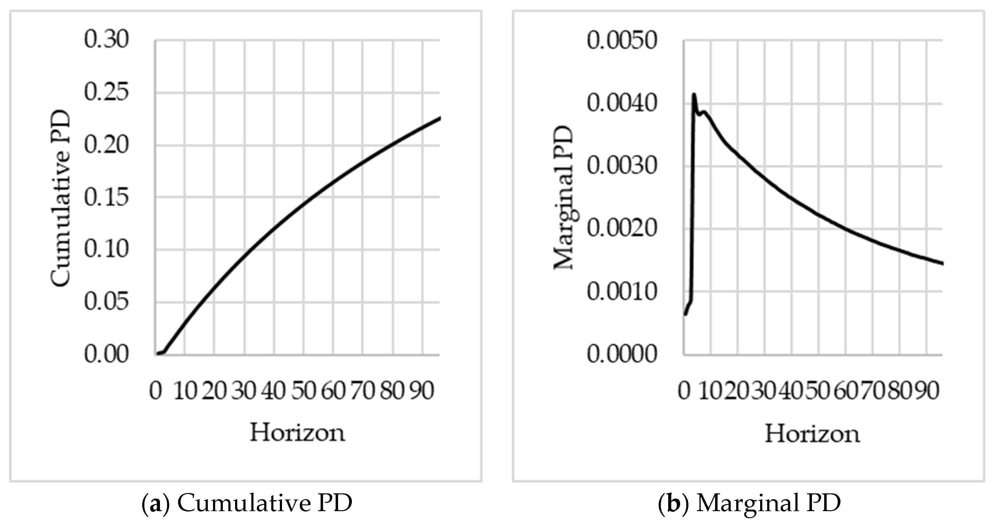
This section describes how marginal PDs (referred to as ‘PD term structures’ in future) are derived by using empirical information. The method creates PD term structures based on the most recent default information and accounts’ risk characteristics prior to default. The approach accounts for attrition effects (i.e., accounts closing from a performing status and can thus no longer default in subsequent months) such that no separate adjustment will be required in the calculation of ECL. The proposed methodology also includes re-default events in the PD term structures (i.e., scenarios where an account defaulted more than once during its lifetime) such that lifetime PDs can theoretically exceed 100% for high risk accounts, particular for portfolios with long lifetime assumptions. This approach was chosen to capture the portfolio’s actual default behaviour more accurately and reduce complexities compared to a ‘worst ever’ modelling approach, typically used in regulatory models. The same approach must also be applied in the LGD model, e.g., by assigning a zero loss assumption to cure events to avoid double counting effects. Different PiT PD term structures are developed to capture the structurally different default risk patterns for different pools of accounts using segmentation.
To define the PD term structure, we define the cumulative and marginal PD’s similarly as in (
Yang 2017). Let
be the cumulative PD for the period (
with respect to observation month
i.e., the probability of defaulting in the total period (
. We define the marginal PD in the period
with respect to observation month
is then defined as
. Note that by definition, for the period
we have
.
To estimate the empirical marginal PD’s we construct a defaults table containing the number of defaults and performing accounts. Each row in the defaults table represents an observation month, where is the set of observation months e.g., {201501, 201502, …, 201507}. Let be the number of accounts that were performing as at the observation month , and then defaulted in the period months after the observation month and the number of performing accounts that survived in the period , where is the number of months since the observation month , i.e., will be the number of performing accounts as at the observation month.
Table 1 is an illustrative example of the defaults table. The number of performing accounts at the start of the observation month 201501 (i.e.,
) was 500 accounts (i.e.,
). Of these 500 accounts 10 accounts defaulted in 201502, during the period
(i.e.,
), and 5 accounts defaulted in 201503, during the period
(i.e.,
). Note that no forecasting is required.
From the defaults table, the empirical PD’s, per observation month
can be calculated as follow:
After having derived the empirical marginal PD estimates for the different observation months and outcome horizons , it needs to be decided which of these estimates should contribute to the final PD term structure and how these contributions should be weighted. As mentioned earlier, the model’s objective is to yield PiT PD estimates such that only defaults from the most recent outcome months are used in the final PD estimates. is referred to as the ‘reference period’ and is a key parameter for estimating the PD term structure. A shorter reference period will make the resulting estimates more PiT but could result in unwanted volatility (and vice versa for longer reference periods). If one uses a very long reference period over an entire economic cycle, the resulting PD term structures can be considered to provide through-the-cycle (TTC) estimates. It may sometimes also be required not to use the most recent data, e.g., if models are refreshed in August but should only account for information until June. Hence, a reference month is used in order to denote the last observation month from the set of observations months that is used in the derivation of . Therefore only defaults from the outcome months are used for modelling purposes.
We estimated the marginal PD, , from the defaults table, as the weighted average of marginal PDs across the most recent observation months with available outcome horizons of at least months. A weighting by the number of observations is performed to smooth the impact of outlier months for segments with small and volatile population sizes.
Thus given
and a reference month
(note that the term structure is generally calculated taking the reference month to be the most recent observation month, i.e.,
) we estimate the marginal PD for time horizon
as
For example, if a reference period of 3 months is chosen (
and the reference month is 201507 (
, then
Table 2 illustrates the resulting marginal PDs.
To summarise, the approach will create PD term structures based on the most recent default information and initial performing accounts as at observation month. It does not require the explicit modelling of future cures or closures, as no survival analysis is required. Below we discuss how the PD term structure is segmented.
Segmentation of PD Term Structures
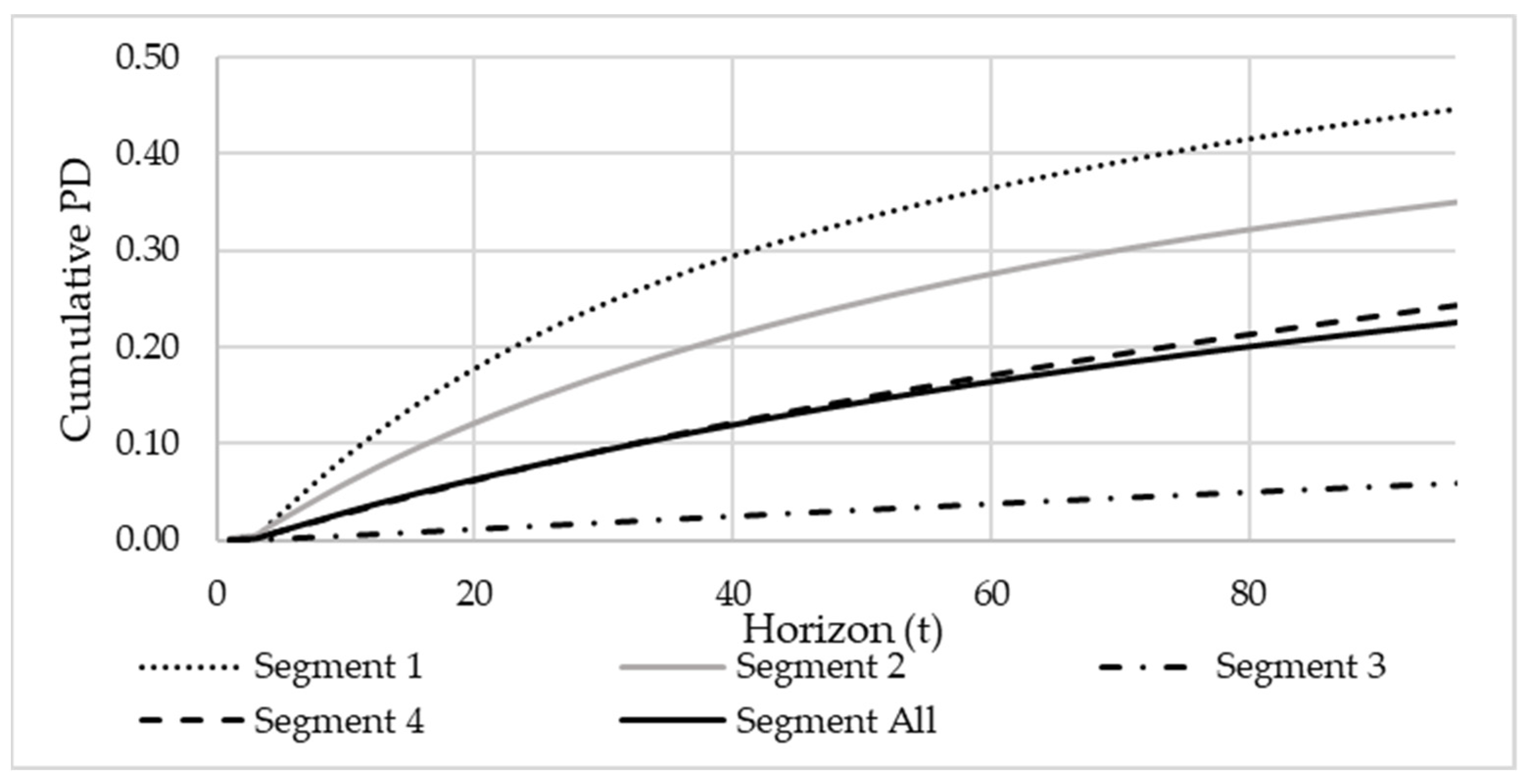
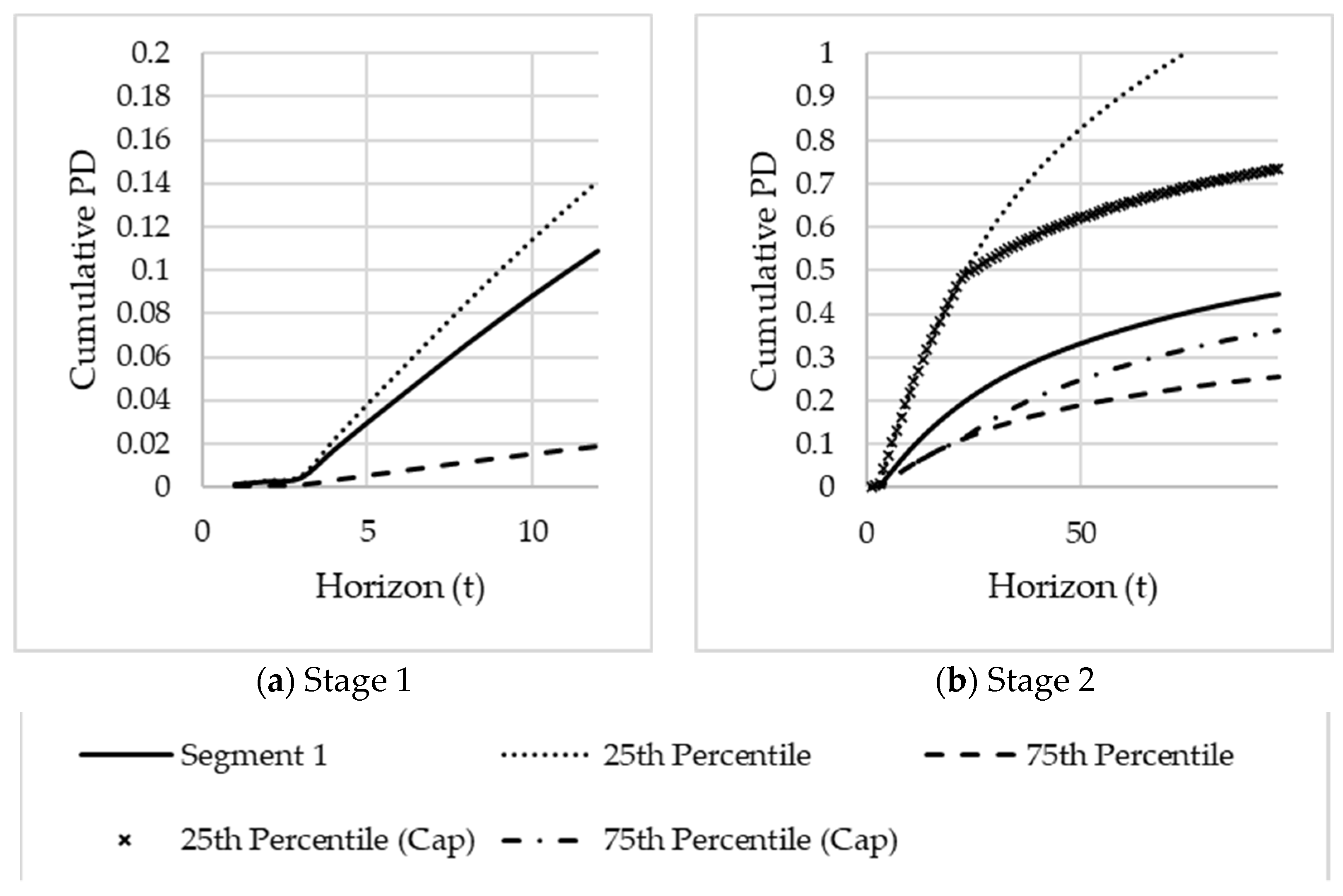
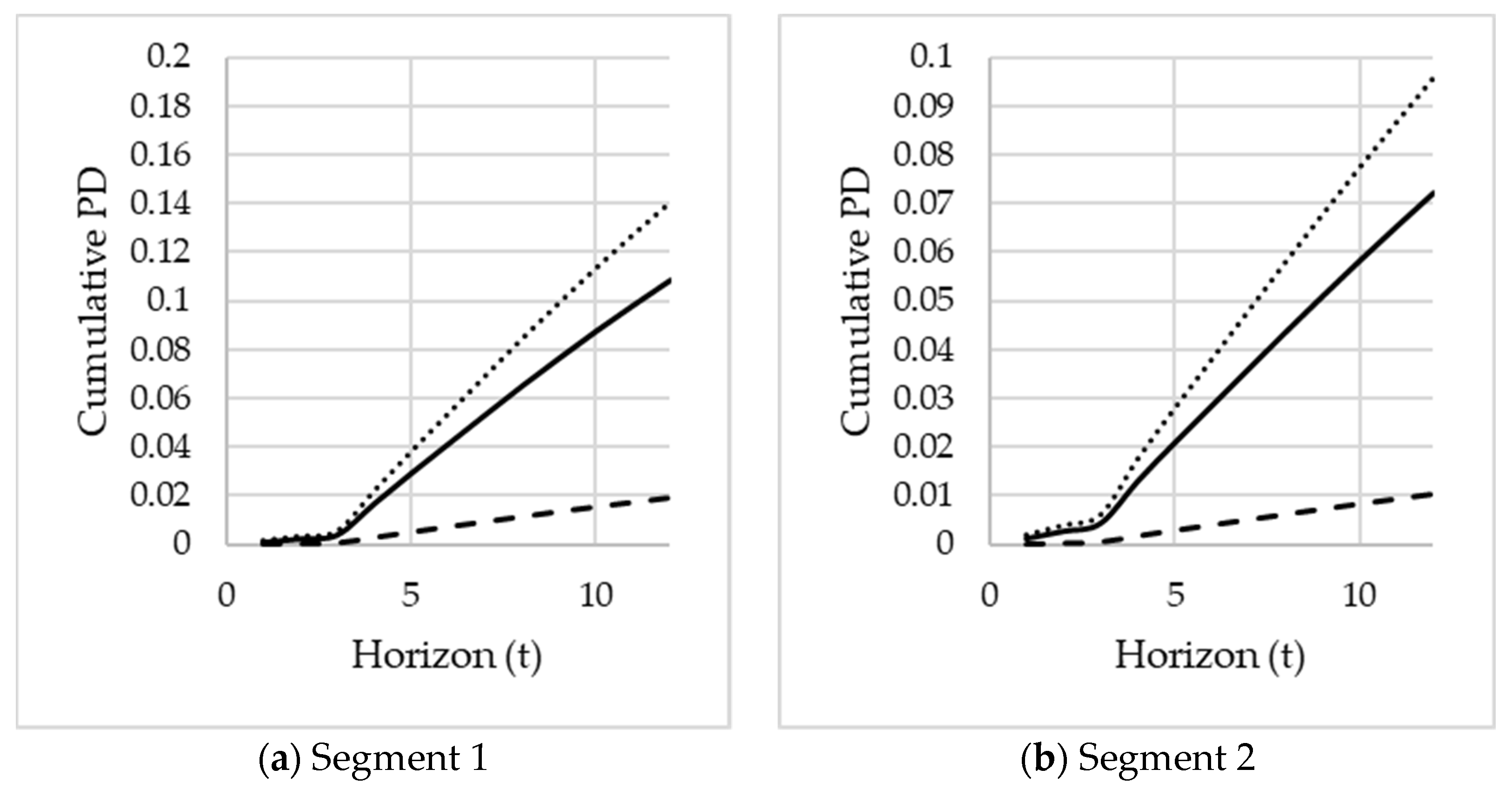
We have a single PD term structure at this stage, and typically, a revolving retail credit portfolio is not a homogeneous set of exposures. Hence, it is unlikely that a single PD term structure would adequately fit across different pools of accounts. If the portfolio is left unsegmented, then the resulting PD term structure will represent a combination of low risk PD term structures and high risk PD term structures. Such an unsegmented PD term structure will understate the default risk of high risk customers and overstate the default risk of low risk customers. Typical examples of effects that cause PD term structures to be materially different from a portfolio average are ageing effects and irregular payment behaviours. Young accounts tend to carry significant default risk in the first year or two after origination, but this improves significantly over time.
In contrast, more matured accounts do not show this significant further improvement in later time periods. Customers with irregular payment behaviour in the recent past have a higher risk of defaulting shortly after observation than in later periods, while very low risk customers often show a more constant (or even increasing) default risk over time. Therefore, a steep increasing cumulative PD term structure is needed for the high risk customers, whereas a more linear-shaped cumulative PD term structure would be needed for the low risk customers.
Therefore, it is necessary to identify segments for which the PD term structure shape is structurally different from the shape of the unsegmented PD term structure to ensure an appropriate risk differentiation. Banks commonly segment their portfolios along business lines, product types and risk characteristics to model more homogeneous loans groups (
McPhail and McPhail 2014). To identify these segments, detailed data analysis based on typical dimensions like delinquency cycle, account age or product type is used and often supported by additional insights from business areas.
It is also important to quantify what a materially different term structure constitutes. To assess whether segmented PD term structures are materially different from the corresponding unsegmented PD term structure, the following tests are proposed:
Visual comparison of the segmented PD term structures vs the unsegmented PD term structure: The segmented PD term structures should ideally show no crossings and provide clear risk differentiation.
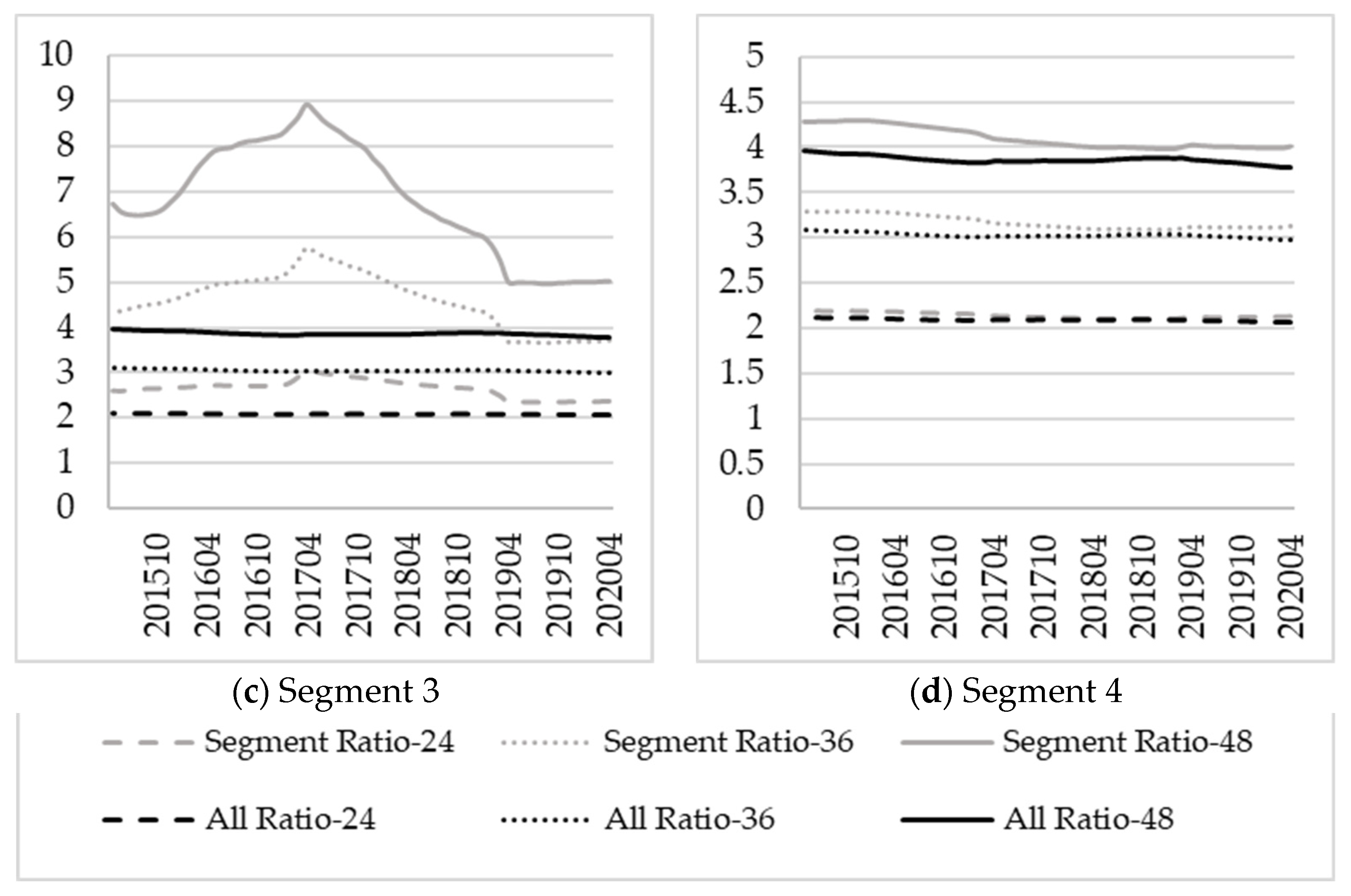
Comparing the ratio of cumulative segmented PDs over different horizons to the 12 month cumulative segmented PD: Define for months. These ratios assess the segmented PD term structure’s steepness. The ratios will also show potential levels of over- or underestimations if only the unsegmented PD term structure is used. The ratios can be analysed over time by varying the reference month .
Comparison of the cumulative segmented PDs to cumulative unsegmented PDs over time for different horizons: This test will confirm whether the difference between the segmented PD term structures and the unsegmented one remains consistent over different horizons months. The PDs can be analysed over time by varying the reference month .
The validity of the suggested segments will be evaluated using these three tests. These three tests are another contribution to this paper and will be illustrated in the case study.
3.2. Account-Specific Term Structures Using Lorenz Curve Calibration
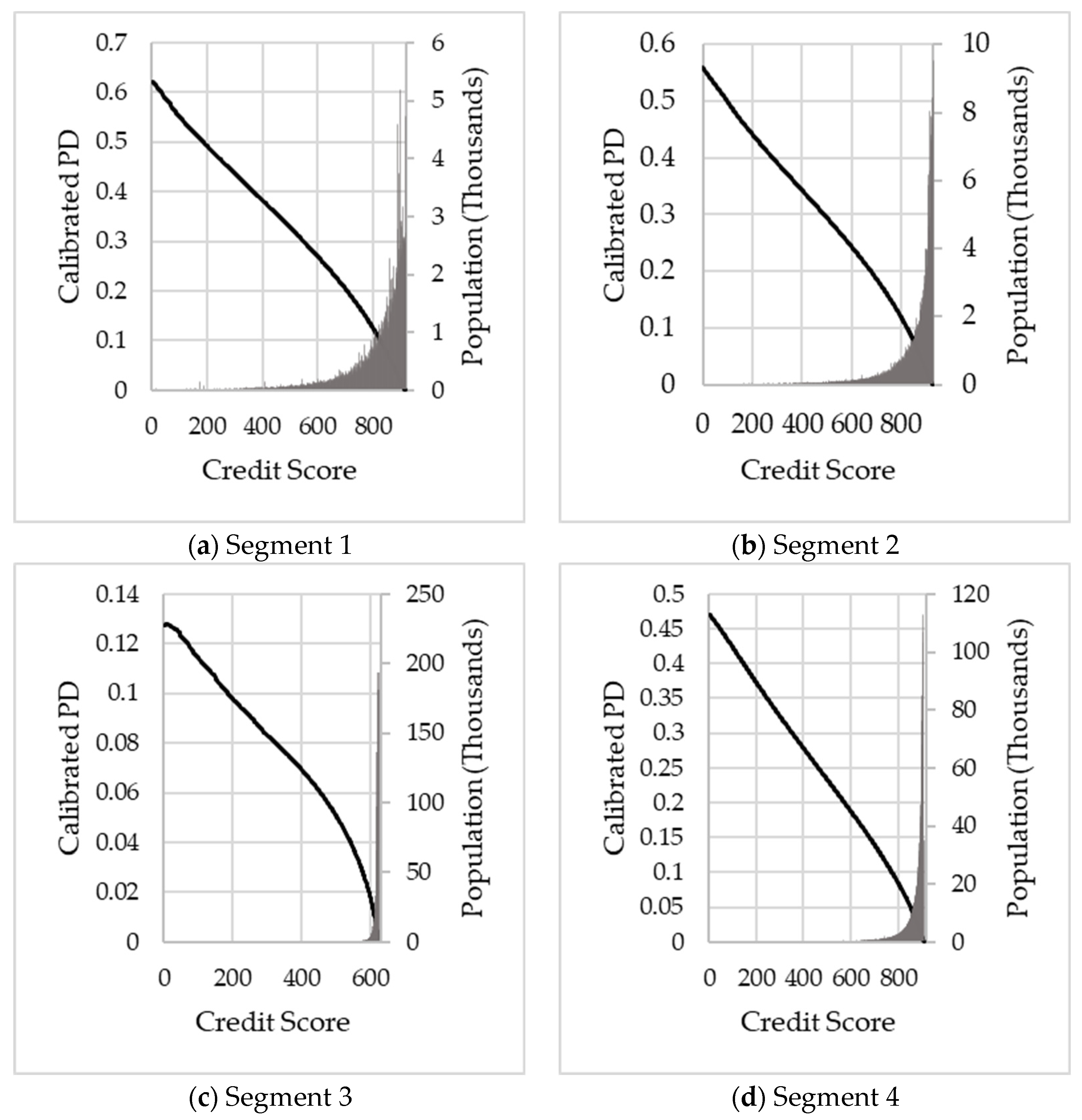
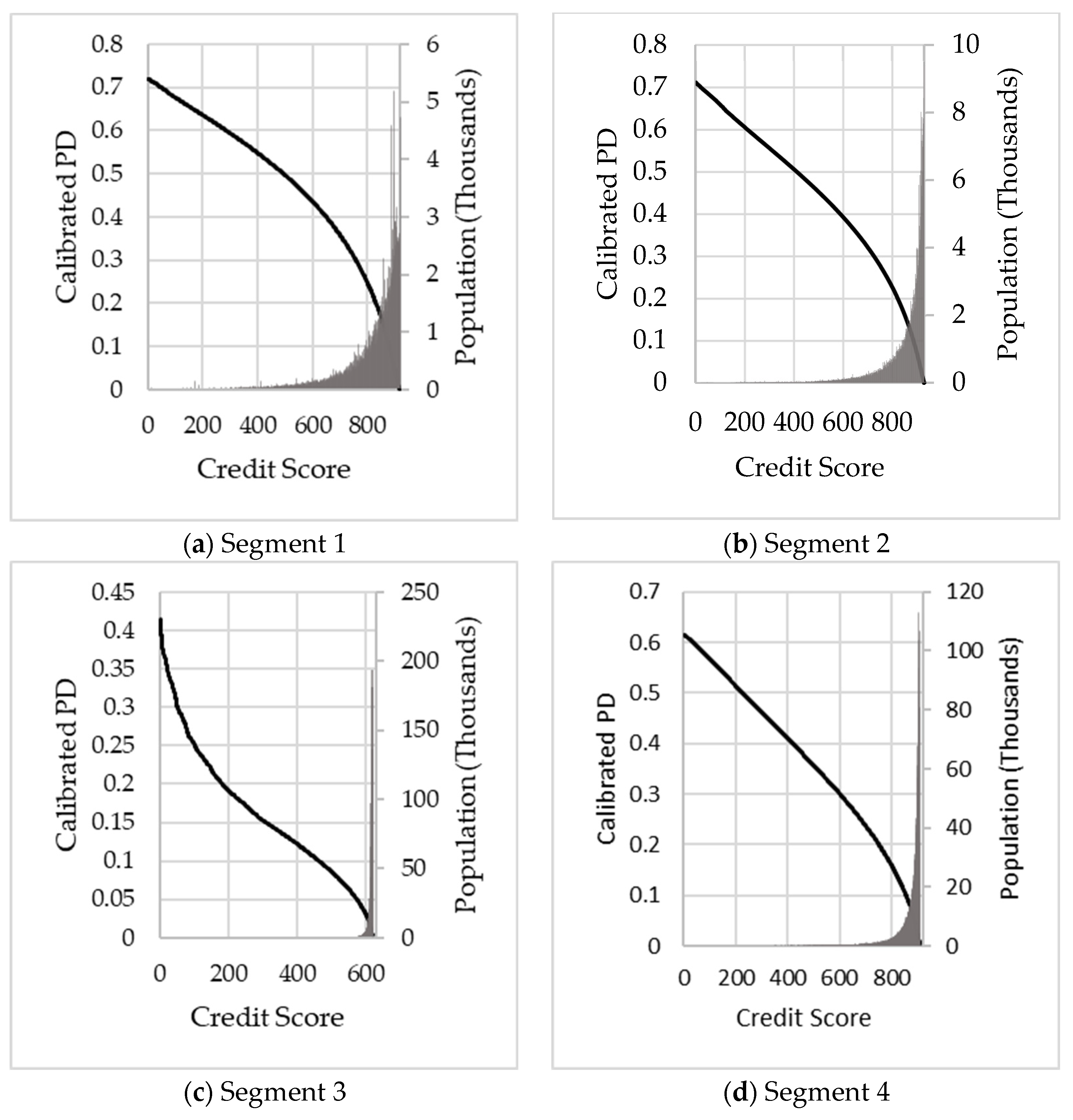
Until now, segment level granularity has been achieved, but more granularity is required to estimate the IFRS 9 PiT PD accurately. In this section, a methodology is proposed to yield account level granularity for the PD estimates. The credit score, in conjunction with a calibration technique, will be used. Any type of credit score that yields good risk differentiation can be used for this approach. Behavioural scores typically provide the best predictive power for revolving retail credit portfolios. In this paper, we used the Lorenz curve as the calibration method (
Glößner 2003). Once the base PD term structures are created using the methodology described in
Section 3.1, account specific PiT PDs will be derived through the Lorenz curve calibration using the latest default experience together with the credit scores. Two PD term structures are created for each account, one to be used for Stage 1 ECL calculations and the other to be used for Stage 2 ECL calculations. Note that separate calibrations will be required for different segments used for the base PD term structures to improve the calibrated PDs. The key two reasons for performing this extra step post the creation of the base PD term structures are as follows:
To obtain more granular PD term structures per credit score, which will increase the accuracy of account level ECL estimates as well as the identification of Stage 2 accounts for which the default risk has significantly increased since origination; and
To make average PD estimates more point-in-time by accounting for changes in score levels.
Assume two cumulative distribution functions
and
, where
is the cumulative distribution of defaulted accounts and
is the cumulative distribution of all accounts for credit score
. The Lorenz curve is defined as the graphical plot of the proportion of defaulted accounts against the proportion of all accounts. Mathematicaly the Lorenz curve is defined by
Glößner (
2003) as:
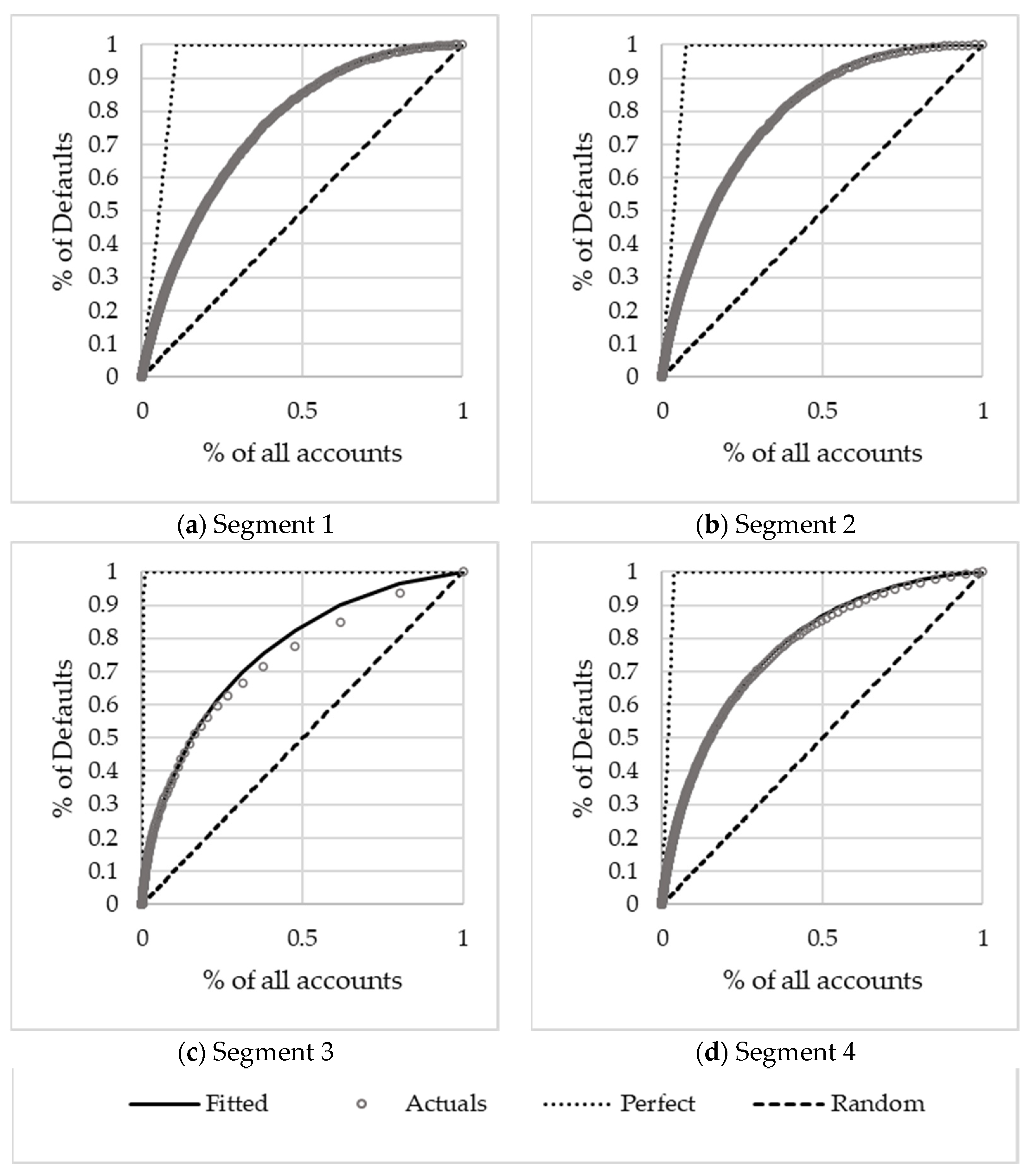
An example of a Lorenz curve (solid line) is shown in
Figure 1. The
-axis of the Lorenz curve indicates the cumulative proportion of all accounts, and the
-axis the cumulative proportion of defaulted accounts. Suppose the defaulted accounts are distributed evenly across scores amongst the portfolio. In that case, the
y fraction is more or less equal to the
x fraction in which case the resulting Lorenz curve would be the 45-degree diagonal (dashed line), indicating that the credit score
has no distinguishing power. The other extreme would be a credit score
separating the good accounts from the bad ones perfectly (dotted line). In this case, the Lorenz curve runs linearly to
, until the
value equal to the percentage of defaulted accounts is reached and stays there.
The Lorenz curve can be used to estimate the cumulative PD, over a horizon
, for accounts with a given credit score
(
Glößner 2003). The estimated PD of accounts with a given credit score
is the fraction of defaulted accounts with a credit score
of all accounts with a credit score
, i.e.,
, where
the density of defaulted accounts and
the density of all accounts for credit score
.
Glößner (
2003) further shows the cumulative PD, over a horizon
, is also:
where
is the average PD over the whole portfolio.
Specific invariancy properties (
Glößner 2003) of the Lorenz curve make this method a stable way to estimate PDs. Considerably less information is needed to fit a numerically constructed Lorenz curve than to fit the two numerical distributions it is constructed from. When applying the Lorenz curve, we make the following two assumptions:
The validity of the calculated PD relies on the account’s scoring results, i.e., distinguishing power of the credit score used; and
The density functions and are assumed to be lognormal.
The ensure lognormality assumption the credit score is transformed (see
Glößner 2003) using different transformations. Assume
refers to a transformation applied to the credit score
with a score range [
] where
and
are the minimum and the maximum observed credit scores.
Glößner (
2003) proves the Lorenz curve’s transformation invariance and proposes three possible transformations: the quadratic, exponential and logarithm.
By assuming that the densities
and
are lognormal, the cumulative PD over a horizon
can be estimated from the data as:
where
and
are lognormal CDFs of the transformed credit scores for defaulted and all accounts, respectively, with parameters
and
.
is the average PD estimated from the data.
The parameters may be estimated from the same data as in
Table 1. For example, to construct a three month cumulative PD from the data in
Table 1, over an observation period of three months,
Table 3 gives an example of the data required to construct the Lorenz curve.
Furthermore, consider a scoring range between 1 and 3 with 1 unit between each score, where 1 is the worst score and 3 is the best score. The number of performing accounts and cumulative defaulted accounts,
, are determined for each score in the dataset, as illustrated in
Table 4.
The average PD of the portfolio
is estimated as
, where
and
.
is any subset of
, the observation period (i.e., sample window) and
the horizon (i.e., the performance window) over which the Lorenz curve is calibrated. The parameters
and
for the calibrated Lorenz curve
, can be estimated by minimising the sum of squares of differences to the empirical Lorenz curve. The point wise-defined empirical Lorenz curve is
The resulting objective function is
The choice of transformation
is motivated by the specific transformation applied to the credit score that minimises the sum of squared differences (SSD) between the calibrated Lorenz curve and the empirical Lorenz curve (
Glößner 2003).
A Gini can be calculated to determine how well the calibrated PDs differentiate between the defaulted accounts and all accounts. Note that the calibration has no impact on the Gini as it does not change the rank order. The Gini statistic (
Siddiqi 2006) quantifies a model’s ability to discriminate between two possible values of a binary target variable (
Tevet 2013). Cases are ranked according to the predictions, and the Gini then provides a measure of predictive power. It is one of the most popular retail credit scoring measures (
Baesens et al. 2016) and has the added advantage that it is a single value (
Tevet 2013). For detailed Gini calculations, the reader can consult various literature sources, e.g.,
SAS Institute (
2017) and
Breed et al. (
2019).
To create an account specific PiT PD term structure for a given performance window
(e.g., 12 months for Stage 1) a scaling factor is calculated as:
where
the cumulative Lorenz curve calibrated
month PD for an account with credit score
and
the cumulative
month term structure PD. The resulting marginal PD for accounts with a credit score
in the period
] is then defined as
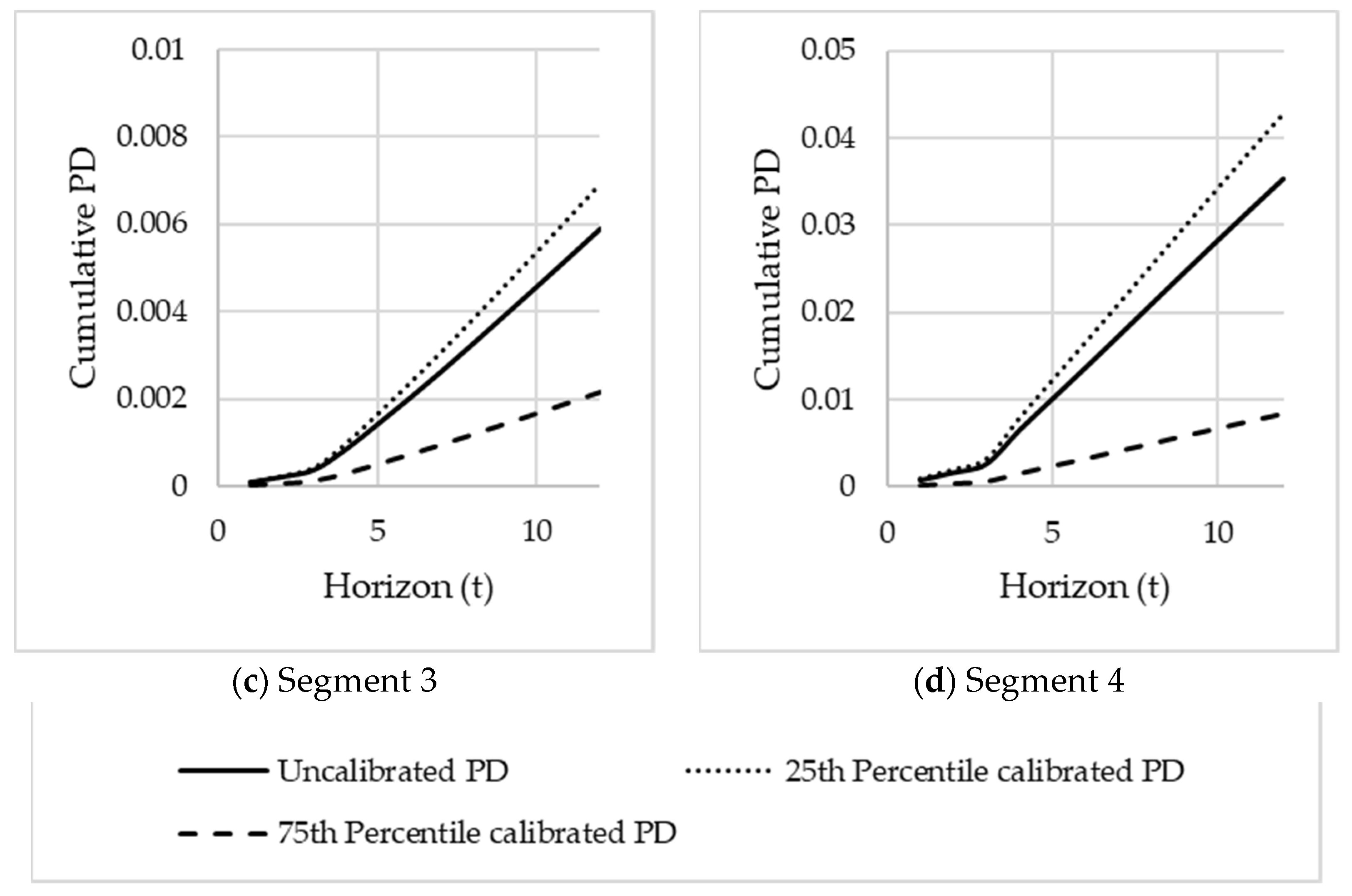
This approach ensures that the cumulative PD assigned to a customer corresponds to his calibrated PD. For Stage 1 and Stage 2, two Lorenz curve calibrations are required. For Stage 1, the ECL is calculated over a 12 month period and therefore .
To illustrate, let’s assume Customer A and Customer B are in the same segment (i.e., the same term structure) but with different credit scores (). Customer A has a scaling factor of 0.76 ( and Customer B has a scaling factor of 1.22 (). Suppose we assume a marginal PD in the period of the PD term structure for the segment to which Customer A and B belong, is 2.3%. In that case, the resulting marginal PD of Customer A will be 1.748% (2.3% × 0.76) and for Customer B 2.806% (2.3% × 1.22).
For Stage 2, a lifetime ECL is calculated, and the choice of the performance window
will depend on the product type, quality of data and expected lifetime
Typically for Stage 2
, since the confidence in the Lorenz curve calibration becomes lower for longer performance windows. With
the resulting marginal lifetime PDs may be unrealistically high (or low) for horizons
due to the wide range of calibrated PDs. Therefore, only the marginal PD for accounts with a credit score
in the period
, for
are adjusted, and the remainder stays unchanged:
This approach ensures that the average predicted lifetime PD remains aligned to actual default behaviour in the respective segment.

