The Weak Convergence Rate of Two Semi-Exact Discretization Schemes for the Heston Model

Abstract

Inspired by the article Weak Convergence Rate of a Time-Discrete Scheme for the Heston Stochastic Volatility Model, Chao Zheng, SIAM Journal on Numerical Analysis 2017, 55:3, 1243–1263, we studied the weak error of discretization schemes for the Heston model, which are based on exact simulation of the underlying volatility process. Both for an Euler- and a trapezoidal-type scheme for the log-asset price, we established weak order one for smooth payoffs without any assumptions on the Feller index of the volatility process. In our analysis, we also observed the usual trade off between the smoothness assumption on the payoff and the restriction on the Feller index. Moreover, we provided error expansions, which could be used to construct second order schemes via extrapolation. In this paper, we illustrate our theoretical findings by several numerical examples.

1. Introduction and Main Results

The Heston Model Heston (1993) is a widely used stochastic volatility model to price financial options. It consists of two stochastic differential equations (SDEs) for an asset price process S and its volatility V:

$$\begin{array}{c}\hfill \begin{array}{cc}\hfill d{S}_t& =\mu S_{t}dt+\sqrt{V_t}{S}_t\left(\rho d{W}_t+\sqrt{1-{\rho }^2}d{B}_t\right),\hfill \\ \hfill d{V}_t& =\kappa (\theta -V_t)dt+\sigma \sqrt{V_t}d{W}_t,\hfill \end{array}\end{array}$$

(1)

with $S_0,V_0,\kappa ,\theta ,\sigma >0$, $\mu \in \mathbb{R}$, $\rho \in [-1,1]$, $T>0$ and independent Brownian motions $W={\left(W_t\right)}_{t\in [0,T]}$, $B={\left(B_t\right)}_{t\in [0,T]}$, which are defined on a filtered probability space $(\mathsf{\Omega },\mathcal{F},{\left({\mathcal{F}}_t\right)}_{t\in [0,T]},\mathbb{P})$, where the filtration satisfies the usual conditions. It is a simple and popular extension of the Black–Scholes model where the volatility of the asset was assumed to be constant. As a consequence, the Heston Model takes the asymmetry and excess kurtosis of financial asset returns into account which are typically observed in real market data. The volatility is given by the so-called Cox–Ingersoll–Ross process (CIR). Its Feller index $\nu =\frac{2\kappa \theta }{{\sigma }^2}$ will be an important parameter for our results. Throughout this article, the initial values $S_0$, $V_0$ are assumed to be deterministic.

To price options with maturity at time T, one is interested in the value of

$$\begin{array}{c}\hfill \mathbb{E}\left[g\left(S_T\right)\right],\end{array}$$

where $g:[0,\infty )\to \mathbb{R}$ is the payoff function. Closed formulae for $\mathbb{E}\left[g\left(S_T\right)\right]$ are rarely known and often Monte Carlo methods are applied, for which in turn the simulation of $S_T$ is required. Usually, the log-Heston model instead of the Heston model is considered in numerical practice. This yields the SDE

$$\begin{array}{c}\hfill \begin{array}{cc}\hfill d(log\left(S_t\right))& =(\mu -\frac{1}{2}{V}_t)dt+\sqrt{V_t}d\left(\rho W_t+\sqrt{1-{\rho }^2}{B}_t\right),\hfill \\ \hfill d{V}_t& =\kappa (\theta -V_t)dt+\sigma \sqrt{V_t}d{W}_t,\hfill \end{array}\end{array}$$

(2)

and the exponential is then incorporated in the payoff, i.e., g is replaced by $f:\mathbb{R}\to \mathbb{R}$ with $f\left(x\right)=g(exp(x\left)\right)$.

While exact simulation schemes and their refinements are known (see, e.g., Broadie and Kaya (2006); Glasserman and Kim (2011); Malham and Wiese (2013); Smith (2007)), discretization schemes as, e.g., Altmayer and Neuenkirch (2017); Andersen (2008); Kahl and Jäckel (2006); Lord et al. (2009), are very popular for the Heston model. The latter discretization schemes can be easily extended to the multi-dimensional case and avoid computational bottlenecks of the exact schemes. In particular, Euler-type methods, such as the fully truncated Euler scheme, seem to be very efficient (see, e.g., Coskun and Korn (2018); Lord et al. (2009)), but no weak error analysis is available for them, up to the best of our knowledge.

A second order discretization scheme for the log-Heston model has been introduced in Andersen (2008) and analyzed in Zheng (2017). The so-called Broadie-Kaya trick and a removal of the drift, detailed in Section 3.1, reduce the simulation of the log-Heston model to the joint simulation of

$$\begin{array}{c}\hfill \begin{array}{cc}\hfill d{X}_t& =\left(\frac{\rho \kappa }{\sigma }-\frac{1}{2}\right)V_{t}dt+\sqrt{1-{\rho }^2}\sqrt{V_t}d{B}_t,\hfill \\ \hfill d{V}_t& =\kappa (\theta -V_t)dt+\sigma \sqrt{V_t}d{W}_t.\hfill \end{array}\end{array}$$

(3)

Moreover, since the transition density of the CIR process $V={\left(V_t\right)}_{t\in [0,T]}$ follows a non-central chi-square distribution, it can be simulated exactly. Trapezoidal discretizations of the first component $X={\left(X_t\right)}_{t\in [0,T]}$ lead to the trapezoidal scheme

$$\begin{array}{cc}\hfill x_{k+1}=x_k& +\left(\frac{\rho \kappa }{\sigma }-\frac{1}{2}\right)\frac{v_{k+1}+v_k}{2}(t_{k+1}-t_k)\hfill \\ & +\sqrt{1-{\rho }^2}\sqrt{\frac{v_{k+1}+v_k}{2}}{\Delta }_{k}B,k=0,\dots ,N-1,\hfill \end{array}$$

where $0=t_0<\dots <t_k<\dots <t_N=T$, $v_k=V_{t_k}$ and ${\Delta }_{k}B=B_{t_k+1}-B_{t_k}$. This discretization avoids in particular the cumbersome exact simulation of the integrated volatility. Zheng (2017) establishes weak order two for polynomial test functions by transferring the error analysis to that of a trapezoidal rule for multidimensional deterministic integrals. Our original intention was to extend this result to a larger class of test functions f by using the Kolmogorov PDE approach. However, the required Itō-Taylor expansions turned out to be not feasible. So, instead, we analyzed the following two semi-exact discretization schemes: the Euler-type scheme

$$\begin{array}{c}\hfill x_{k+1}=x_k+\left(\frac{\rho \kappa }{\sigma }-\frac{1}{2}\right)v_k(t_{k+1}-t_k)+\sqrt{1-{\rho }^2}\sqrt{v_k}{\Delta }_{k}B\end{array}$$

(4)

and the semi-trapezoidal scheme

$$\begin{array}{c}\hfill x_{k+1}=x_k+\left(\frac{\rho \kappa }{\sigma }-\frac{1}{2}\right)\frac{v_{k+1}+v_k}{2}(t_{k+1}-t_k)+\sqrt{1-{\rho }^2}\sqrt{v_k}{\Delta }_{k}B.\end{array}$$

(5)

In both schemes, the CIR process is simulated exactly. In our opinion, the analysis of these schemes gives valuable insights in the weak error analysis of discretization schemes for the log-Heston model and is also a good starting point for the analysis of full Euler-type discretization schemes.

Our error analysis relies on two regularity results for the Heston PDE (Briani et al. (2018); Feehan and Pop (2013)), the Kolmogorov PDE approach for the weak error analysis from Talay and Tubaro (1990), and Malliavin calculus. We also observe the usual trade off between the smoothness assumption on the payoff and the restriction on the Feller index. For payoffs of lower smoothness, a restriction on the Feller index $\nu =2\kappa \theta /{\sigma }^2$ is required, which arises from the use of Malliavin calculus tools.

In the following, we use the notation

$$\Delta t=\underset{k=1,\dots ,N}{max}|t_k-t_{k-1}|$$

for the maximal step size and the usual notations for the spaces of differentiable functions. In particular, the subscript c denotes compact support and $pol$ denotes polynomial growth. In addition, see Section 3.1. The results of Feehan and Pop (2013) require compact support of the test functions f, while the results of Briani et al. (2018) allow polynomial growth but require higher smoothness for f.

Theorem 1.

Let $\epsilon >0$. (i) If $f\in C_c^{2+\epsilon }(\mathbb{R}\times {\mathbb{R}}_{+};\mathbb{R})$ and $\frac{2\kappa \theta }{{\sigma }^2}>\frac{3}{2}$, then both schemes satisfy

$$\begin{array}{c}\hfill \mathbb{E}\left[f(x_N,v_N)\right]-\mathbb{E}\left[f(X_T,V_T)\right]=O\left(\Delta t\right).\end{array}$$

(ii) If $f\in C_c^{4+\epsilon }(\mathbb{R}\times {\mathbb{R}}_{+};\mathbb{R})$, then both schemes satisfy

$$\begin{array}{c}\hfill \mathbb{E}\left[f(x_N,v_N)\right]-\mathbb{E}\left[f(X_T,V_T)\right]=O\left(\Delta t\right).\end{array}$$

Assuming more smoothness of f, we obtain more detailed results:

Theorem 2.

Suppose that $f\in C_{pol}^8(\mathbb{R}\times {\mathbb{R}}_{+};\mathbb{R})$. (i) Then, the Euler scheme (4) satisfies

$$\begin{array}{c}\hfill \mathbb{E}\left[f(x_N,v_N)\right]-\mathbb{E}\left[f(X_T,V_T)\right]=\sum _{n=0}^{N-1}{\int }_{t_n}^{t_{n+1}}{\int }_{t_n}^t\mathbb{E}\left[\mathcal{H}(s,t,{\widehat{x}}_s,{\widehat{x}}_t,V_s,V_t)\right]dsdt+O({(\Delta t)}^2),\end{array}$$

where

$$\begin{array}{cc}\hfill \mathcal{H}(s,t,{\widehat{x}}_s,{\widehat{x}}_t,V_s,V_t)& =\left(\frac{1}{2}-\frac{\rho \kappa }{\sigma }\right)\left(\kappa (\theta -V_s)u_x(t,{\widehat{x}}_t,V_t)+{\sigma }^2{V}_s{u}_{xv}(s,{\widehat{x}}_s,V_s)\right)\hfill \\ \hfill & -\frac{(1-{\rho }^2)}{2}\left(\kappa (\theta -V_s)u_{xx}(t,{\widehat{x}}_t,V_t)+{\sigma }^2{V}_s{u}_{xxv}(s,{\widehat{x}}_s,V_s)\right)\hfill \end{array}$$

and

$$\begin{array}{cc}\hfill {\widehat{x}}_t& =x_n+\left(\frac{\rho \kappa }{\sigma }-\frac{1}{2}\right)v_n(t-t_n)+\sqrt{1-{\rho }^2}\sqrt{v_n}(B_t-B_{t_n}),t\in [t_n,t_{n+1}],\hfill \end{array}$$

for$n=0,\dots ,N-1$.

In particular, for an equidistant discretization with$t_k=kT/N$, $k=0,\dots ,N$, we have

$$\begin{array}{c}\hfill \underset{N\to \infty }{lim}N\left(\mathbb{E}\left[f(x_N,v_N)\right]-\mathbb{E}\left[f(X_T,V_T)\right]\right)=\frac{T}{2}{\int }_0^T\mathbb{E}\left[\mathcal{H}(t,t,X_t,X_t,V_t,V_t)\right]dt.\end{array}$$

Here, u denotes the solution of the associated Kolmogorov PDE; see Equation (7).

(ii) For the semi-trapezoidal scheme (5), we have

$$\begin{array}{c}\hfill \mathbb{E}\left[f(x_N,v_N)\right]-\mathbb{E}\left[f(X_T,V_T)\right]=\sum _{n=0}^{N-1}{\int }_{t_n}^{t_{n+1}}{\int }_{t_n}^t\mathbb{E}\left[\mathcal{H}(s,t,{\widehat{x}}_s,{\widehat{x}}_t,V_s,V_t)\right]dsdt+O({(\Delta t)}^2),\end{array}$$

where

$$\begin{array}{cc}\hfill \mathcal{H}(s,t,{\widehat{x}}_s,{\widehat{x}}_t,V_s,V_t)& =-\frac{(1-{\rho }^2)}{2}\left(\kappa (\theta -V_s)u_{xx}(t,{\widehat{x}}_t,V_t)+{\sigma }^2{V}_s{u}_{xxv}(s,{\widehat{x}}_s,V_s)\right)\hfill \end{array}$$

and

$$\begin{array}{cc}\hfill {\widehat{x}}_t=x_n& +\left(\frac{\rho \kappa }{\sigma }-\frac{1}{2}\right)\frac{V_t+v_n}{2}(t-t_n)+\sqrt{1-{\rho }^2}\sqrt{v_n}\left(B_t-B_{t_n}\right),t\in [t_n,t_{n+1}],\hfill \end{array}$$

for $n=0,\dots ,N-1$.

In particular, for an equidistant discretization $t_k=kT/N$, $k=0,\dots ,N$, it holds

$$\begin{array}{c}\hfill \underset{N\to \infty }{lim}N\left(\mathbb{E}\left[f(x_N,v_N)\right]-\mathbb{E}\left[f(X_T,V_T)\right]\right)=\frac{T}{2}{\int }_0^T\mathbb{E}\left[\mathcal{H}(t,t,X_t,X_t,V_t,V_t)\right]dt.\end{array}$$

Here, u denotes again the solution of the associated Kolmogorov PDE; see Equation (7).

Thus, the semi-trapezoidal rule eliminates the first two terms of the error expansion of the Euler scheme.

Remarks

Remark 1.

We expect that the error expansions for an equidistant discretization for both schemes satisfy

$$\begin{array}{c}\hfill \mathbb{E}\left[f(x_N,v_N)\right]-\mathbb{E}\left[f(X_T,V_T)\right]=\left(\frac{T}{2}{\int }_0^T\mathbb{E}\left[\mathcal{H}(t,t,x_t,x_t,v_t,v_t)\right]dt\right)·N^{-1}+O\left(N^{-2}\right).\end{array}$$

(6)

However, to establish this, we would require error estimates for functionals of the type $\mathbb{E}\left[f(\lambda ,X_T,V_T)\right]$ with $\lambda \in [0,T]$, which are uniform in λ. (Compare, e.g., Proposition 2 in Talay and Tubaro (1990).) This, in turn, would require uniform regularity estimates for the Heston PDE, which are not available at the moment.

Remark 2.

Property (6) allows to construct a second order scheme via extrapolation: If (6) holds, then

$$Y_N=2f(x_{2N},v_{2N})-f(x_N,v_N)$$

satisfies

$$\mathbb{E}{Y}_N=\mathbb{E}f(X_T,V_T)+O\left({(\Delta t)}^2\right),$$

where $(x_{2N},v_{2N})$ uses the stepsize $T/\left(2N\right)$ and $(x_N,v_N)$ the stepsize $T/N$.

Remark 3.

We require smoothness assumptions for f that are not met by the payoffs in practice, which are at most Lipschitz continuous or even discontinuous. However, this is a typical problem for weak approximation of SDEs as the Heston SDE, which do not satisfy the so-called standard assumptions on the coefficients. In Bally and Talay (1996), only bounded and measurable test functions f are treated assuming uniform hypoellipticity of the coefficients of the SDE. However, the Heston model does not satisfy this property. An adaptation of the strategy of Bally and Talay (1996) to the Heston model yields strong assumption on the Feller index (see Altmayer (2015)), which we want to avoid here.

Remark 4.

Schemes built on the Broadie-Kaya trick, i.e., Equation (3), have a different structure than schemes which arise by a direct discretization of the log-Heston model as, e.g., the schemes studied in Altmayer and Neuenkirch (2017); Lord et al. (2009). For example, the so-called absorbed Euler discretization reads as

$$\begin{array}{cc}\hfill z_{k+1}& =z_k-\frac{1}{2}{v}_k(t_{k+1}-t_k)+\sqrt{v_k}\left(\rho \left(W_{t_{k+1}}-W_{t_k}\right)+\sqrt{1-{\rho }^2}\left(B_{t_{k+1}}-B_{t_k}\right)\right),\hfill \\ \hfill v_{k+1}& ={\left(v_k+\kappa \left(\theta -v_k\right)(t_{k+1}-t_k)+\sigma \sqrt{v_k}\left(W_{t_{k+1}}-W_{t_k}\right)\right)}^{+}.\hfill \end{array}$$

Here, the volatility $V={\left(V_t\right)}_{t\in [0,T]}$ is discretized by an Euler scheme, a fix for retaining the positivity is introduced by using the positive part, and the equation for the log-Heston price $Z={(log\left(S_t\right))}_{t\in [0,T]}$ is discretized instead of the one for $X={\left(X_t\right)}_{t\in [0,T]}$.

Remark 5.

The Broadie-Kaya trick is a particular case of a more general transformation procedure, which has been introduced in Cui et al. (2018) for a general class of stochastic volatility models. In addition, in Cui et al. (2018), the weak convergence of a Markov chain approximation for these equations is established, which had been introduced in Cui et al. (2020). Markov chain approximations have been also studied in Briani et al. (2018) for the Heston and Bates model and are an alternative to a classical discretization of stochastic differential equations. In particular, for pricing American options, they can be beneficial.

2. Numerical Results

In this section, we will test numerically whether the convergence rates for the Euler Scheme (4) and the Semi-Trapezoidal Scheme (5) are attained even under milder assumptions than those from Theorems 1 and 2. We use the following model parameters:

• Model 1: $S_0=100,V_0=0.010201,K=100,\kappa =6.21,\theta =0.019,\sigma =0.61,\rho =-0.7,T=1,r=0.0319$;
• Model 2: $S_0=100,V_0=0.09,K=100,\kappa =2,\theta =0.09,\sigma =1,\rho =-0.3,T=5,r=0.05$;
• Model 3: $S_0=100,V_0=0.0457,K=100,\kappa =5.07,\theta =0.0457,\sigma =0.48,\rho =-0.767,T=2,r=0.00$.

The Feller index is $\nu =\frac{2\kappa \theta }{{\sigma }^2}\approx 0.63$ in Model 1, $\nu \approx 0.36$ in Model 2, and $\nu \approx 2.01$ in Model 3. For each model, we use the following payoff functions:

1.

European Call: $g_1\left(S_T\right)=e^{-rT}max\{S_T-K,0\}$;

2.

European Put: $g_2\left(S_T\right)=e^{-rT}max\{K-S_T,0\}$;

3.

Indicator: $g_3\left(S_T\right)=e^{-rT}{\mathbf{1}}_{[0,K]}\left(S_T\right)$.

Note that none of these payoffs satisfies the assumptions of our Theorems. Thus, the presented numerical experiments explore whether the Theorems are valid under milder assumptions. In order to measure the weak error rate, we simulated $M=2·{10}^7$ independent copies $g_i(s_N^{\left(j\right)})$, $j=1,\dots ,M$, of $g_i\left(s_N\right)$ to estimate

$$\mathbb{E}\left(g_i\left(s_N\right)\right)$$

by

$$p_{M,N}=\frac{1}{M}\sum _{j=1}^M{g}_i(s_N^{\left(j\right)})$$

for each combination of model parameters, functional and number of steps $N\in \{2^1,...,2^6\}$ where $\Delta t=\frac{T}{N}$. The number of Monte Carlo samples is chosen in such a way that the Monte Carlo error is sufficiently small enough, i.e., does not dominate the theoretically expected convergence rates. The Monte Carlo mean of these samples was then compared to a reference solution $p_{\mathsf{ref}}$, i.e.,

$$e\left(N\right)=|p_{\mathsf{ref}}-p_{M,N}|,$$

and the error $e\left(N\right)$ is plotted in Figure 1, Figure 2, Figure 3, Figure 4, Figure 5, Figure 6, Figure 7, Figure 8, Figure 9, Figure 10, Figure 11, Figure 12, Figure 13, Figure 14, Figure 15, Figure 16, Figure 17 and Figure 18. We then measured the rate of convergence, i.e., the decay rate of $e\left(N\right)$, by the slope of a least-squares fit in logarithmic coordinates. The reference solutions can be computed with sufficiently high accuracy from semi-explicit formulae via Fourier methods. In particular, the put price can be calculated from the call-price formula given in Heston (1993) via the put-call-parity. The price of the digital option can be computed from the probability $P_2$ given in Heston (1993); it equals $e^{rT}\left(1-P_2\right)$. Additionally to the Euler and Semi-Trapezoidal scheme, we simulated the Trapezoidal scheme as in Zheng (2017) and the two extrapolation schemes from Remark 2. Moreover, to present a broader picture we estimated the weak error order of two Euler-type discretizations of the full Heston Model, the Full Truncation Euler (FTE) as in Lord et al. 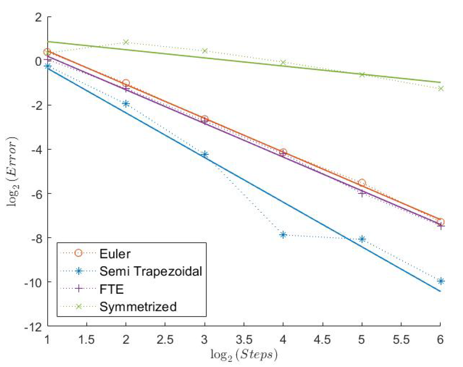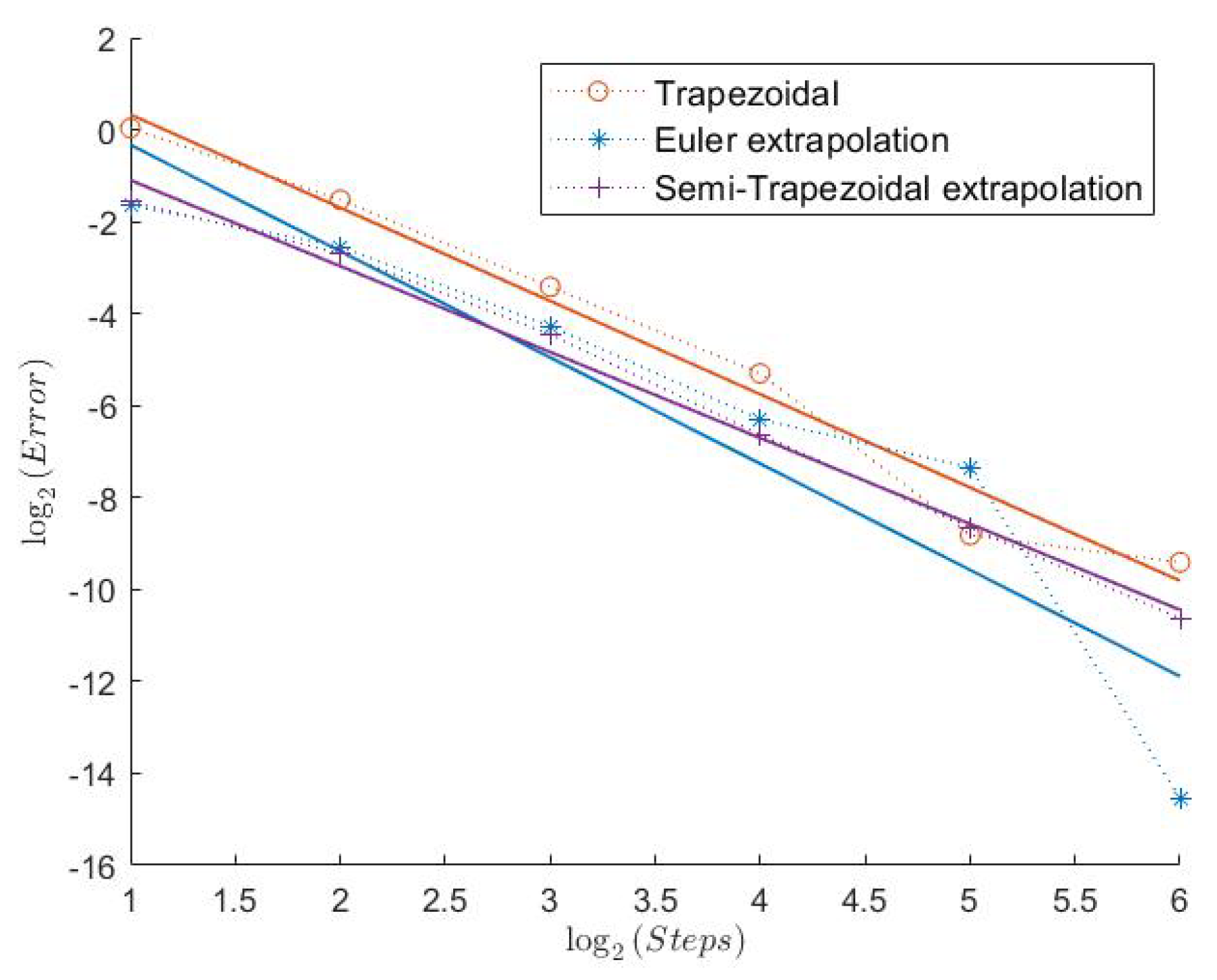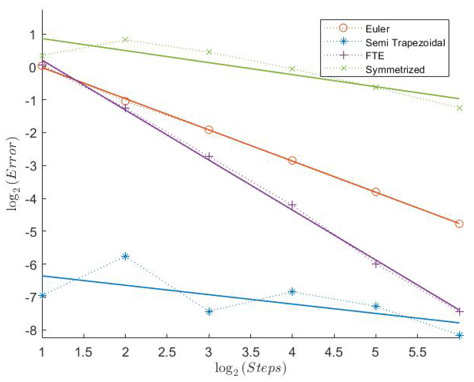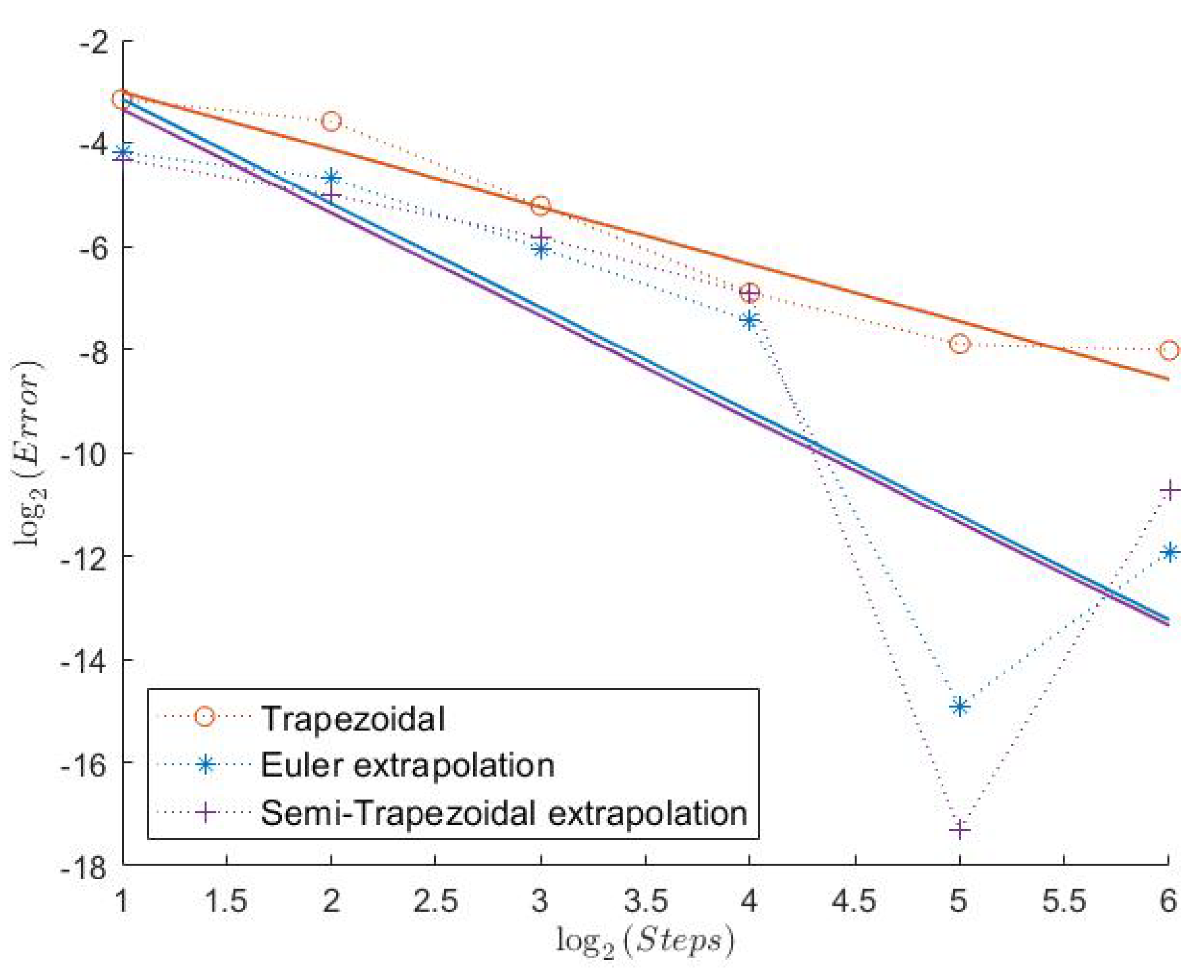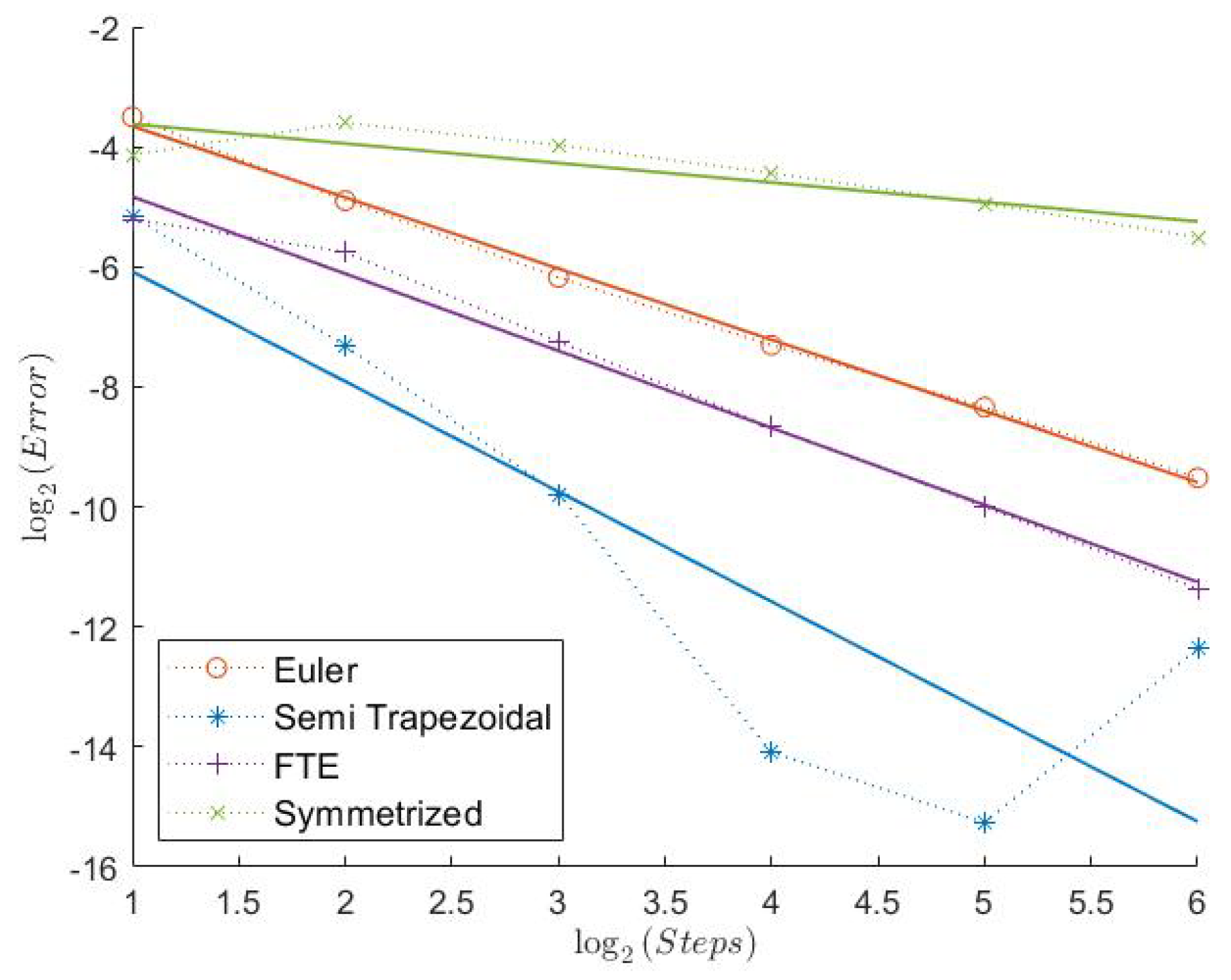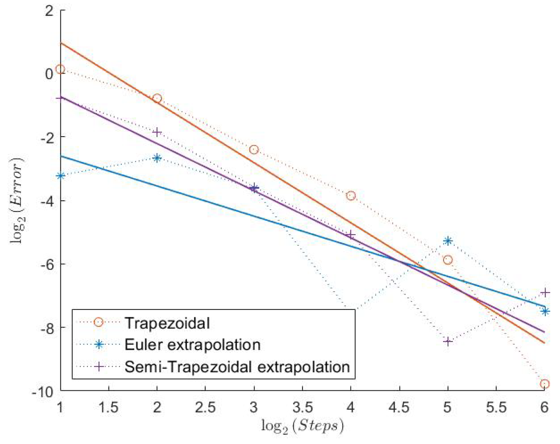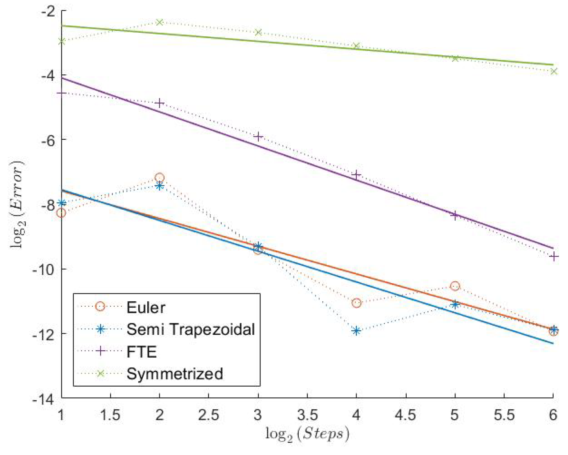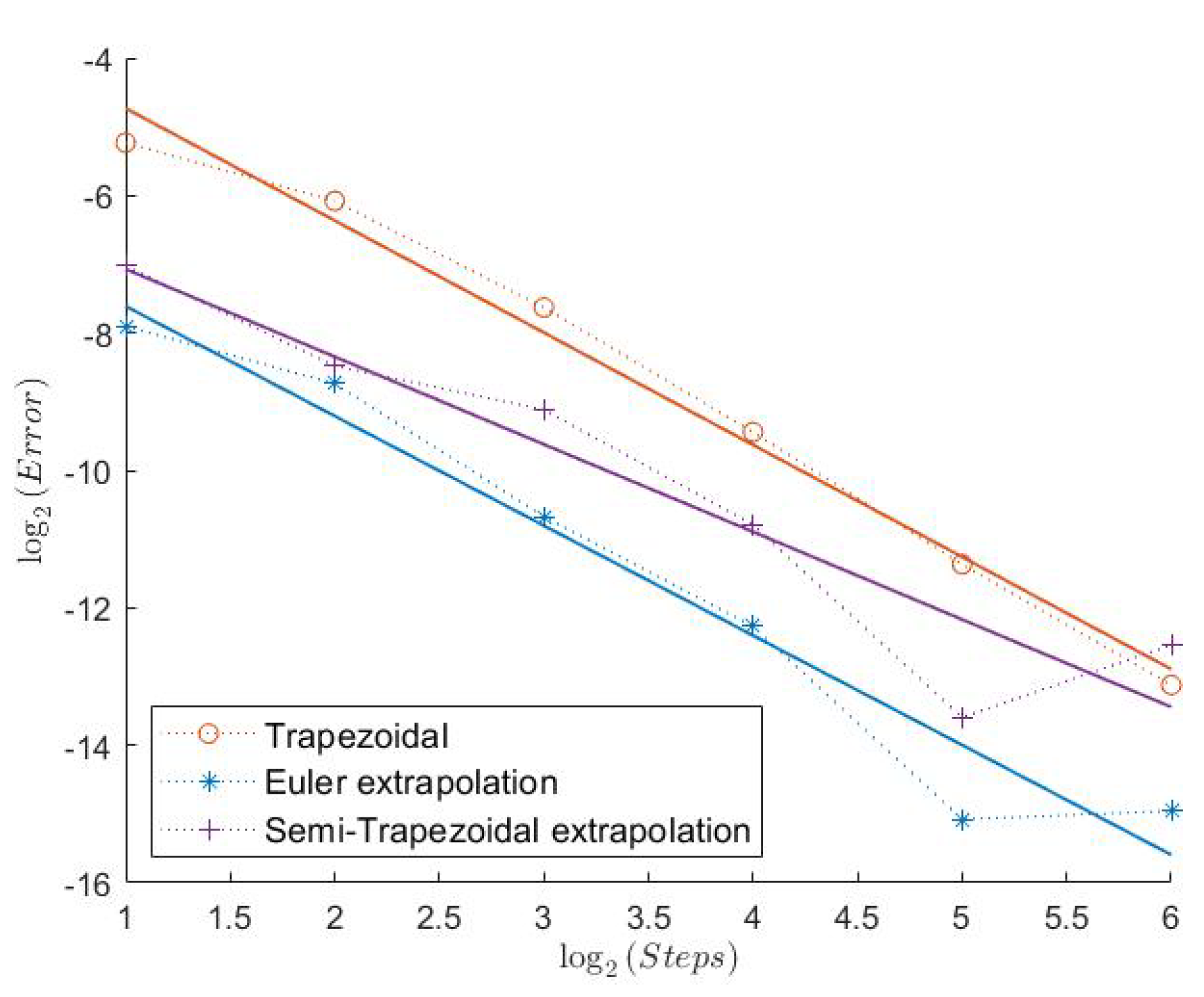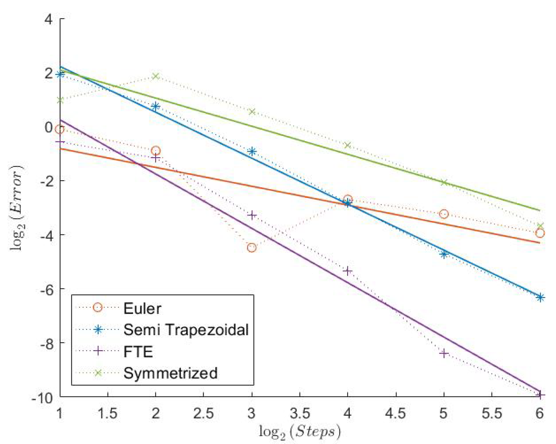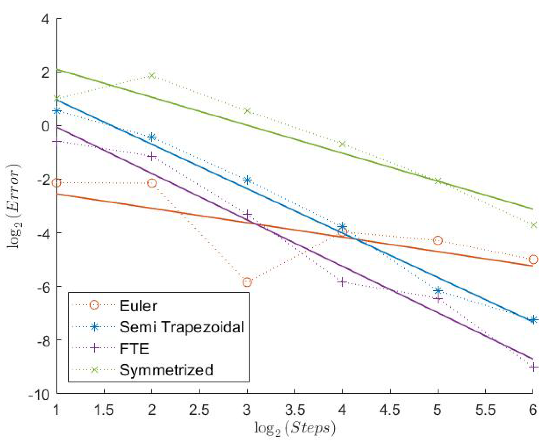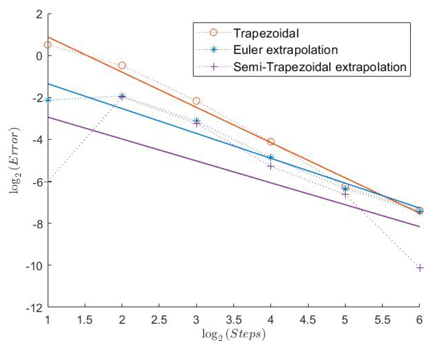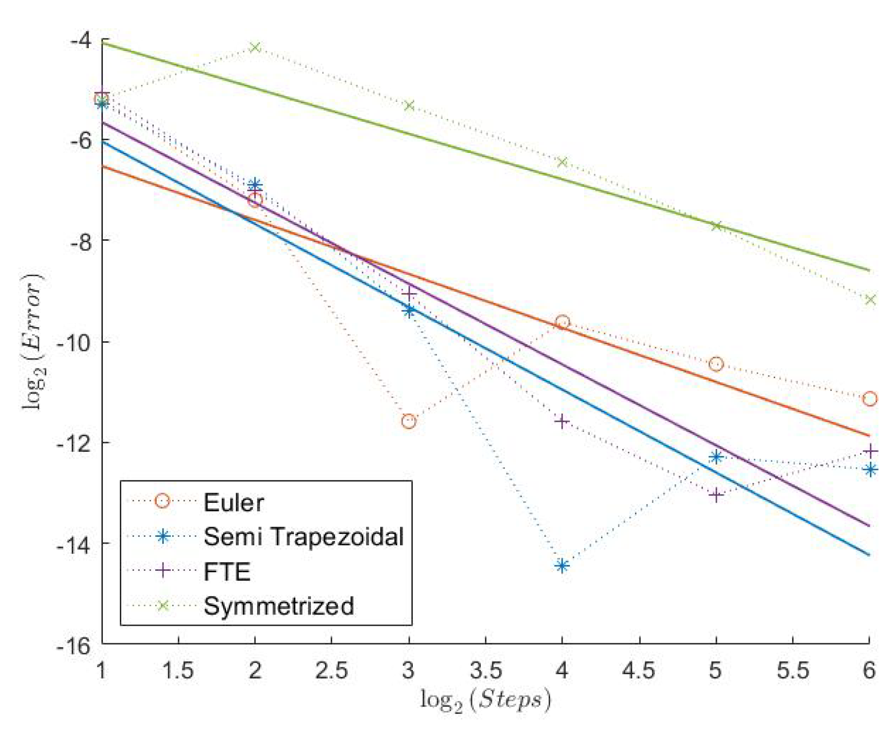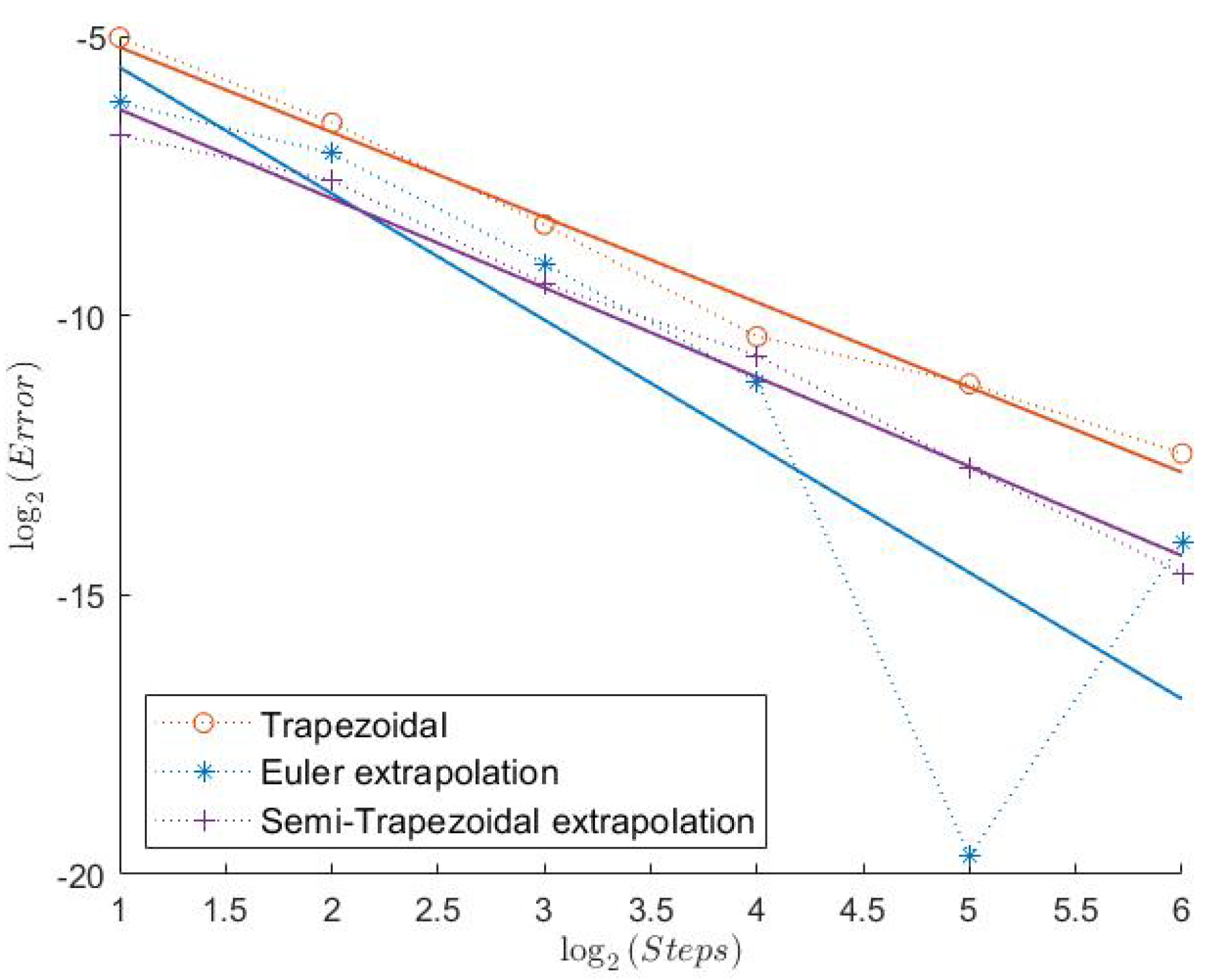(2009), and the Symmetrized Euler as in Bossy and Diop (2015). To clarify things, we show two plots for each combination of model parameters and functional: one with the suspected order one schemes (Euler, Semi-Trapezoidal, FTE, and Symmetrized Euler) and one with the suspected order two schemes (Trapezoidal, Extrapolated Euler, and Extrapolated Semi-Trapezoidal).

Figure 1. Call Model 1.

Figure 2. Call Model 1.

Figure 3. Put Model 1.

Figure 4. Put Model 1.

Figure 5. Indicator Model 1.

Figure 6. Indicator Model 1.

Figure 7. Call Model 2.

Figure 8. Call Model 2.

Figure 9. Put Model 2.

Figure 10. Put Model 2.

Figure 11. Indicator Model 2.

Figure 12. Indicator Model 2.

Figure 13. Call Model 3.

Figure 14. Call Model 3.

Figure 15. Put Model 3.

Figure 16. Put Model 3.

Figure 17. Indicator Model 3.

Figure 18. Indicator Model 3.

2.1. Model 1

In Table 1, we can see the measured convergence rates for this model with a Feller index of $\nu \approx 0.63.$ The associated plots are shown in Figure 1, Figure 2, Figure 3, Figure 4, Figure 5 and Figure 6.

Table 1. Measured convergence rates Model 1.

Method	Call	Put	Indicator
Euler	1.5252	0.9492	1.1870
Semi-Trapezoidal	2.0174	0.2857	1.8343
FTE	1.5205	1.5205	1.2847
Symmetrized Euler	0.3693	0.3659	0.3250
Trapezoidal	2.0283	1.1119	2.4544
Euler extrap.	2.3114	2.0172	1.9719
Semi-Trapezoidal extrap.	1.8687	1.9999	0.9834

All “Order 1” schemes seem to have a very regular convergence behavior except for the Semi-Trapezoidal scheme for the Indicator, which could be explained by the low absolute error. Especially for the Call and the Indicator, both schemes from Theorem 1 seem to have very high weak convergence rates. Because of the Feller index of 0.63 in this model, this indicates that the assertion of Theorems 1 and 2 could hold under weaker assumptions. The extremely low estimated convergence rate for the Semi-Trapezoidal scheme in combination with the Put could be due to the low error. The estimated weak error order of the FTE scheme is noticeably higher than 1, whereas the Symmetrized Euler has low convergence rates. The convergence behavior of the “Order 2” schemes is a bit less regular. The Extrapolated Euler scheme seems to converge with order 2 for all payoff functions, whereas the Extrapolated Semi-Trapezoidal scheme seem to have only order 1 for the Indicator. But, again, we notice that the error for just 2 discretization steps already starts at around 2⁻¹⁰, which is extremely low.

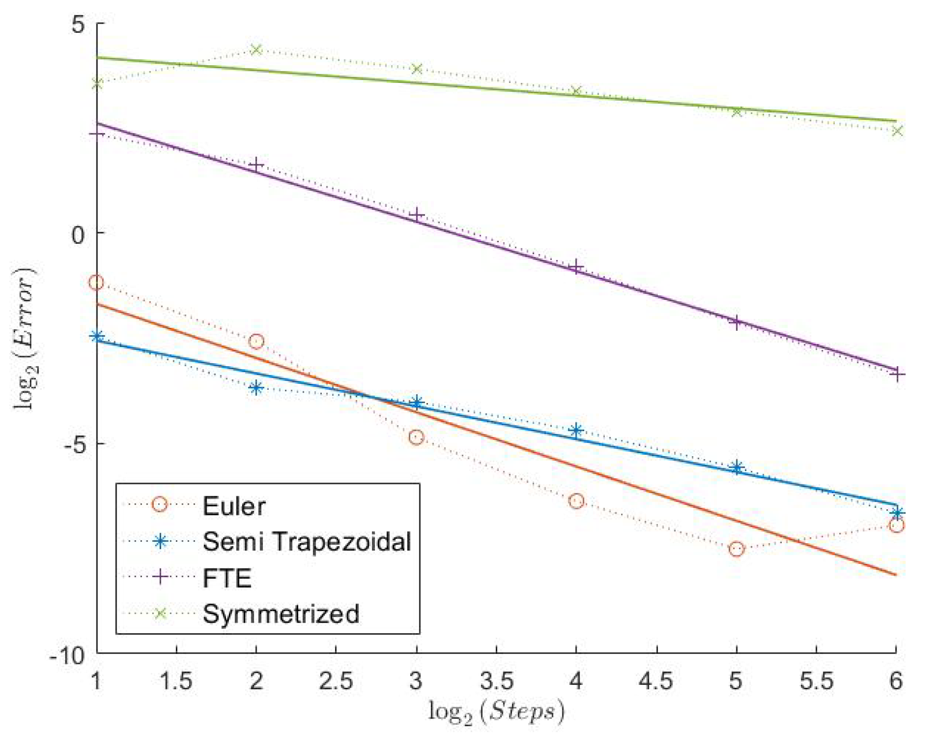
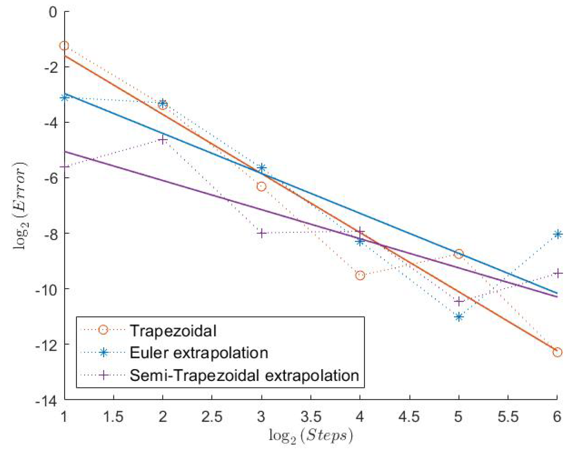
2.2. Model 2

Here, we have an even lower Feller index of $\nu \approx 0.36$. We can see that the estimated convergence rates for all “Order 1” schemes are lower than before, see Table 2. However, the Semi-Trapezoidal scheme and the FTE scheme seem to converge with order 1. The convergence behavior is still quite regular as we can see in Figure 7, Figure 9, and Figure 11. In absolute terms, the errors of the schemes from Theorem 1 are the lowest, especially for Put and Indicator. Looking at the “Order 2” schemes, the Trapezoidal discretization still shows an estimated weak convergence rate of around 2, whereas the two extrapolation schemes show a weaker performance. But, especially for the Indicator, all three schemes seem to have a very low error and a quite regular convergence behavior.

Table 2. Measured convergence rates Model 2.

Method	Call	Put	Indicator
Euler	0.4335	1.2898	0.8565
Semi-Trapezoidal	1.3025	0.7810	0.9518
FTE	1.2050	1.1733	1.0546
Symmetrized Euler	0.3028	0.3021	0.2421
Trapezoidal	1.8925	2.1272	1.6324
Euler extrap.	0.9483	1.4393	1.5966
Semi-Trapezoidal extrap.	1.4840	1.0481	1.2744

2.3. Model 3

Here, we have the highest Feller Index with $\nu \approx 2.01$. It is, therefore, a bit surprising that the Euler scheme seems to have a convergence rate of less than 1 in this case. In general, the errors for the “Order 1” schemes show a more irregular behavior, as can be seen from Figure 13, Figure 15, and Figure 17. The Semi-Trapezoidal and the FTE scheme work especially well in this scenario as we can see in Table 3. This is also the only case where the Symmetrized Euler shows an estimated convergence order of around 1. The extrapolation definitely improves the convergence rate of the Euler scheme with order 2 for the Indicator, but this is not the case for the Semi-Trapezoidal scheme.

Table 3. Measured convergence rates Model 3.

Method	Call	Put	Indicator
Euler	0.6977	0.5378	1.0695
Semi-Trapezoidal	1.6989	1.6551	1.6396
FTE	2.0091	1.7303	1.6008
Symmetrized Euler	1.0386	1.0426	0.9018
Trapezoidal	1.8682	1.6799	1.5219
Euler extrap.	1.1612	1.1857	2.2612
Semi-Trapezoidal extrap.	1.5660	1.0441	1.5979

2.4. Computational Times

The computational times show the expected behavior, i.e., the simulation times for the semi-exact schemes increase as the Feller index decreases. See Table 4 and Table 5. This is a well known feature of the MATLAB-generator ncx2rnd for the non-central chi-square distribution, which we used. (All simulations were carried out in MATLAB.)

Table 4. Computational times (sec.) of the semi-exact schemes for 2⁶ time steps and 2 × 10⁷ paths.

Model	1	2	3
Euler	345.73	755.19	145.40
Semi-Trapezoidal	344.53	757.93	144.79
Trapezoidal	342.51	766.01	143.39
Euler extrap.	690.36	2335.94	307.62
Semi-Trapezoidal extrap.	686.55	2371.67	310.29

Table 5. Computational times (sec.) of Euler-type discretizations for 2⁶ time steps and 2 × 10⁷ paths.

Model	1	2	3
FTE	142.3	138.37	141.53
Symmetrized Euler	141.64	140.98	141.67

2.5. Conclusions

Except for the Euler scheme for the Call in Model 3, the simulation studies support the conjecture that the convergence rates of Theorems 1 and 2 hold under weaker assumptions. For the mentioned behavior of the Euler scheme, we do not have an explanation, except the possibly pre-asymptotic step sizes. For the extrapolated schemes, which might have order two, the situation is less clear. Since the behavior of the trapezoidal scheme is regular, a too large Monte Carlo error seems an unlikely explanation. Explanations could be again the pre-asymptotic step sizes or, in fact, the non-smoothness of the considered payoffs.

3. Auxiliary Results

In this section, we will collect and establish, respectively, several auxiliary results for the weak error analysis.

3.1. Kolmogorov PDE

Recall that the stochastic integral equations for the log-Heston model for $0\le s<t\le T$ read as

$$\begin{array}{cc}\hfill log\left(S_t\right)& =log\left(S_s\right)+{\int }_s^t\left(r-\frac{1}{2}{V}_u\right)du+{\int }_s^t\sqrt{V_u}d\left(\rho W_u+\sqrt{1-{\rho }^2}{B}_u\right),\hfill \\ \hfill V_t& =V_s+{\int }_s^t\kappa (\theta -V_u)du+\sigma {\int }_s^t\sqrt{V_u}d{W}_u.\hfill \end{array}$$

Now, we apply the so-called Broadie-Kaya trick from Broadie and Kaya (2006). We can rearrange the second equation:

$$\begin{array}{c}\hfill {\int }_s^t\sqrt{V_u}d{W}_u=\frac{1}{\sigma }\left(V_t-V_s-\kappa \theta (t-s)+\kappa {\int }_s^t{V}_{u}du\right).\end{array}$$

Then, we plug this equation into the first one:

$$\begin{array}{ll}log\left(S_t\right)-log\left(S_s\right)=\frac{\rho }{\sigma }\left(V_t-V_s-\kappa \theta (t-s)+r(t-s)\right)& +\left(\frac{\rho \kappa }{\sigma }-\frac{1}{2}\right){\int }_s^t{V}_{u}du\\ & +\sqrt{1-{\rho }^2}{\int }_s^t\sqrt{V_u}d{B}_u.\end{array}$$

Without loss of generality, we can neglect the non-integral part in $log\left(S_t\right)-log\left(S_s\right)$, since we have

$$f(log\left(S_T\right),V_T)=f\left(X_T+\frac{\rho }{\sigma }\left(V_T-V_0-\kappa \theta T+rT\right),V_T\right)$$

with $X_T=X_T^{0,log\left(S_0\right),V_0}$ given below. To get the Kolmogorov backward PDE, we look at the following integral equations:

$$\begin{array}{cc}\hfill V_t^{s,v}& =v+{\int }_s^t\kappa (\theta -V_r^{s,v})dr+\sigma {\int }_s^t\sqrt{V_r^{s,v}}d{W}_r,\hfill \\ \hfill X_t^{s,x,v}& =x+\left(\frac{\rho \kappa }{\sigma }-\frac{1}{2}\right){\int }_s^t{V}_r^{s,v}dr+\sqrt{1-{\rho }^2}{\int }_s^t\sqrt{V_r^{s,v}}d{B}_r.\hfill \end{array}$$

We set

$$\begin{array}{cc}\hfill u(t,x,v)& =\mathbb{E}\left[f\left(X_T^{t,x,v},V_T^{t,v}\right)\right],t\in [0,T],x\in \mathbb{R},v\ge 0\hfill \end{array}$$

and obtain for $f:\mathbb{R}\times [0,\infty )\to \mathbb{R}$ bounded and continuous the Kolmogorov backward PDE by an application of the Feynman-Kac Theorem (see, e.g., Theorem 5.7.6 in Karatzas and Shreve (1991)):

$$\begin{array}{cc}\hfill u_t(t,x,v)=& -\left(\frac{\rho \kappa }{\sigma }-\frac{1}{2}\right)v{u}_x(t,x,v)-\kappa (\theta -v)u_v(t,x,v)\hfill \\ \hfill & -\frac{v}{2}\left(\left(1-{\rho }^2\right)u_{xx}(t,x,v)+{\sigma }^2{u}_{vv}(t,x,v)\right),t\in (0,T),x\in \mathbb{R},v>0,\hfill \\ \hfill u(T,x,v)=& f(x,v),x\in \mathbb{R},v\ge 0.\hfill \end{array}$$

(7)

In our error analysis, we will follow the now classical approach of Talay and Tubaro (1990), which exploits the regularity of the Kolmogorov backward PDE. For the latter we will rely on the works of Feehan and Pop (2013) and Briani et al. (2018). To state these regularity results, we will need the following notation:

For a multi-index $l=(l_1,...,l_d)\in {\mathbb{N}}^d$, we define $\left|l\right|={\sum }_{j=1}^d{l}_j$ and for $y\in {\mathbb{R}}^d$, we define ${\partial }_y^l={\partial }_{y_1}^{l_1}\dots {\partial }_{y_d}^{l_d}$. Moreover, we denote by $\left|y\right|$ the standard Euclidean norm in ${\mathbb{R}}^d$. Let $\mathcal{D}\subset {\mathbb{R}}^d$ be a domain and $q\in \mathbb{N}$. The set $C^q\left(\mathcal{D};\mathbb{R}\right)$ is the set of all real-valued functions on $\mathcal{D}$ which are q-times continuously differentiable. For $\epsilon \in (0,1)$, we denote by $C^{q+\epsilon }\left(\mathcal{D};\mathbb{R}\right)$ the set of all functions from $C^q\left(\mathcal{D};\mathbb{R}\right)$ in which partial derivatives of order q are Hölder-continuous of order $\epsilon$, and $C_c^{q+\epsilon }\left(\mathcal{D};\mathbb{R}\right)$ is the set of all functions from $C^{q+\epsilon }\left(\mathcal{D};\mathbb{R}\right)$, who have compact support. Moreover, $C_{pol}^q\left(\mathcal{D};\mathbb{R}\right)$ is the set of functions $g\in C^q\left(\mathcal{D};\mathbb{R}\right)$ such that there exist $C,a>0$ for which

$$\begin{array}{c}\hfill |{\partial }_y^l{g\left(y\right)|\le C(1+\left|y\right|}^a),y\in \mathcal{D},|l|\le q.\end{array}$$

Finally, we denote by $C_{pol,T}^q\left(\mathcal{D};\mathbb{R}\right)$ the set of functions $v\in C_{pol}^{\lfloor q/2\rfloor ,q}\left([0,T)\times \mathcal{D};\mathbb{R}\right)$ such that there exist $C,a>0$ for which

$$\begin{array}{c}\hfill \underset{t<T}{sup}|{\partial }_t^k{\partial }_y^l{v(t,y)|\le C(1+\left|y\right|}^a),y\in \mathcal{D},2k+|l|\le q.\end{array}$$

The work of Feehan and Pop deals with general degenerated parabolic equations and establishes a-priori regularity estimates for them. In the context of Equation (7), the main result of Feehan and Pop (2013), i.e., Theorem 1.1, reads as follows:

Theorem 3.

Let $\epsilon >0$ and $f\in C_c^{2+\epsilon }(\mathbb{R}\times {\mathbb{R}}_{+};\mathbb{R})$. Then, there exists a constant $c>0$, depending only on $f,T,\rho ,\kappa ,\theta$ and σ such that the solution u of PDE (7) satisfies

$$\begin{array}{cc}\hfill & \underset{(t,x,v)\in [0,T]\times \mathbb{R}\times [0,\infty )}{sup}\left(\left|u(t,x,v)\right|+|{\partial }_{t}u(t,x,v)|+|{\partial }_{v}u(t,x,v)|+|{\partial }_{x}u(t,x,v)|\right)\le c,\hfill \\ \hfill & \underset{(t,x,v)\in [0,T]\times \mathbb{R}\times [0,1]}{sup}\left(|v{\partial }_{xx}u(t,x,v)|+|v{\partial }_{xv}u(t,x,v)|+|v{\partial }_{vv}u(t,x,v)|\right)\le c,\hfill \\ \hfill & \underset{(t,x,v)\in [0,T]\times \mathbb{R}\times [1,\infty )}{sup}\left(|{\partial }_{xx}u(t,x,v)|+|{\partial }_{xv}u(t,x,v)|+|{\partial }_{vv}u(t,x,v)|\right)\le c.\hfill \end{array}$$

So, under the above assumptions on f, the solution u and the first order derivatives are bounded. Moreover, the second order derivatives are also bounded, if they are damped by v for $v\in [0,1]$.

Assuming more smoothness on f, we can achieve more regularity for u using the above result, at least for the partial derivatives with respect to x. Set

$$\begin{array}{cc}\hfill \widehat{u}(t,x,v)& :=u_x(t,x,v)=\mathbb{E}\left[f_x(X_T^{t,x,v},V_T^{t,v})\right],\hfill \\ \hfill \tilde{u}(t,x,v)& :=u_{xx}(t,x,v)=\mathbb{E}\left[f_{xx}(X_T^{t,x,v},V_T^{t,v})\right].\hfill \end{array}$$

This is well defined: by continuity and boundedness of $f_x$ and dominated convergence we have

$$\begin{array}{cc}\hfill u_x(t,x,v)& =\frac{\partial }{\partial x}\mathbb{E}\left[f(X_T^{t,x,v},V_T^{t,v})\right]=\frac{\partial }{\partial x}\mathbb{E}\left[f(x+Z_T^{t,v},V_T^{t,v})\right]\hfill \\ \hfill & =\underset{\delta \to 0}{lim}\mathbb{E}\left[\frac{f(x+\delta +Z_T^{t,v},V_T^{t,v})-f(x+Z_T^{t,v},V_T^{t,v})}{\delta }\right]\hfill \\ \hfill & =\underset{\delta \to 0}{lim}{\int }_0^1\mathbb{E}\left[f_x(x+\delta \lambda +Z_T^{t,v},V_T^{t,v})\right]d\lambda \hfill \\ \hfill & ={\int }_0^1\mathbb{E}\left[f_x(x+Z_T^{t,v},V_T^{t,v})\right]d\lambda \hfill \\ \hfill & =\mathbb{E}\left[f_x(x+Z_T^{t,v},V_T^{t,v})\right]=\mathbb{E}\left[f_x(X_T^{t,x,v},V_T^{t,v})\right]\hfill \end{array}$$

with

$$\begin{array}{c}\hfill Z_T^{t,v}=\left(\frac{\rho \kappa }{\sigma }-\frac{1}{2}\right){\int }_s^t{V}_r^{s,v}dr+\sqrt{1-{\rho }^2}{\int }_s^t\sqrt{V_r^{s,v}}d{B}_r.\end{array}$$

An analogous calculation for $u_{xx}(t,x,v)$ shows that $u_{xx}(t,x,v)=\mathbb{E}\left[f_{xx}(X_T^{t,x,v},V_T^{t,v})\right]$. Thus, $u_{xx}$ is also bounded, if $f\in C_c^{2+\epsilon }(\mathbb{R}\times {\mathbb{R}}_{+};\mathbb{R})$. Moreover, $\widehat{u}$ fulfills the Kolmogorov backward PDE

$$\begin{array}{cc}\hfill {\widehat{u}}_t(t,x,v)=& -\left(\frac{\rho \kappa }{\sigma }-\frac{1}{2}\right)v{\widehat{u}}_x(t,x,v)-\kappa (\theta -v){\widehat{u}}_v(t,x,v)\hfill \\ \hfill & -\frac{v}{2}\left(\left(1-{\rho }^2\right){\widehat{u}}_{xx}(t,x,v)+{\sigma }^2{\widehat{u}}_{vv}(t,x,v)\right),t\in (0,T),x\in \mathbb{R},v>0,\hfill \\ \hfill \widehat{u}(T,x,v)=& f_x(x,v),x\in \mathbb{R},v\ge 0,\hfill \end{array}$$

while $\tilde{u}$ fulfills the same PDE with terminal condition

$$\begin{array}{cc}\hfill \tilde{u}(T,x,v)=& f_{xx}(x,v),x\in \mathbb{R},v\ge 0.\hfill \end{array}$$

Applying Theorem 3 now to $\widehat{u}$ and $\tilde{u}$, we obtain the following additional bounds (case (ii)) for the derivatives of u:

Corollary 1.

(i) Let $\epsilon >0$ and $f\in C_c^{2+\epsilon }(\mathbb{R}\times {\mathbb{R}}_{+};\mathbb{R})$. Then, there exists a constant $c>0$, depending only on $f,T,\rho ,\kappa ,\theta$ and σ such that the solution u of PDE (7) satisfies

$$\begin{array}{cc}\hfill & \underset{(t,x,v)\in [0,T]\times \mathbb{R}\times [0,\infty )}{sup}\left|{\partial }_{xx}u(t,x,v)\right|\le c.\hfill \end{array}$$

(ii) Let $\epsilon >0$ and $f\in C_c^{4+\epsilon }(\mathbb{R}\times {\mathbb{R}}_{+};\mathbb{R})$. Then, there exists a constant $c>0$, depending only on $f,T,\rho ,\kappa ,\theta$ and σ such that the solution u of PDE (7) satisfies

$$\begin{array}{cc}\hfill & \underset{(t,x,v)\in [0,T]\times \mathbb{R}\times [0,\infty )}{sup}\left(|{\partial }_{xv}u(t,x,v)|+|{\partial }_{xx}u(t,x,v)|+|{\partial }_{xxv}u(t,x,v)|+|{\partial }_{xxx}u(t,x,v)|\right)\le c.\hfill \end{array}$$

The recent work of Briani et al. is a specialized approach for the log-Bates model, of which the log-Heston model is a particular case. In our setting, they obtain in Proposition 5.3 and Remark 5.4 of Briani et al. (2018) the following:

Theorem 4.

Let $q\in \mathbb{N}$, $q\ge 2$ and suppose that $f\in C_{pol}^{2q}(\mathbb{R}\times {\mathbb{R}}_{+};\mathbb{R})$. Then, the solution u of PDE (7) satisfies $u\in C_{pol,T}^q\left(\mathbb{R}\times {\mathbb{R}}_{+};\mathbb{R}\right)$.

In contrast to the results of Feehan and Pop, the result of Briani et al. requires more smoothness of f but allows polynomial growth instead of compact support.

3.2. Properties of the CIR Process

We recall here the following estimates for the CIR process, which are well known or can be found in Hurd and Kuznetsov (2008).

Lemma 1.

(1) We have

$$\mathbb{E}\left[\underset{t\in [0,T]}{sup}{V}_t^p\right]<\infty$$

for all $p\ge 1$ and

$$\underset{t\in [0,T]}{sup}\mathbb{E}{V}_t^p<\infty iffp>-\frac{2\kappa \theta }{{\sigma }^2}.$$

(2) For all $p\ge 1$, there exist constants $c>0$, depending only on $p,\kappa ,\theta ,\sigma ,T,$ and $V_0$, such that

$$\mathbb{E}|V_t-V_s{|}^p\le c·{|t-s|}^{p/2},s,t\in [0,T].$$

We will need the following bound on the growth of the $L^q$-norm of a specific stochastic integral of the CIR process:

Lemma 2.

For all $q\in \left[2,\frac{4\kappa \theta }{{\sigma }^2}\right)$, it holds that

$$\begin{array}{c}\hfill \underset{t\in [0,T]}{sup}{t}^{-q/2}\mathbb{E}\left[|{\int }_0^t\frac{1}{\sqrt{V_u}}d{B}_u{|}^q\right]<\infty .\end{array}$$

Proof. 

With the Burkholder-Davis-Gundy inequality and the Hölder inequality, we have

$$\begin{array}{cc}\hfill t^{-q/2}\mathbb{E}\left[|{\int }_0^t\frac{1}{\sqrt{V_u}}d{B}_u{|}^q\right]& \le t^{-q/2}\mathbb{E}\left[{\left|{\int }_0^t\frac{1}{V_u}du\right|}^{q/2}\right]\hfill \\ \hfill & \le t^{-q/2}\mathbb{E}\left[{\left({\left|{\int }_0^t{\left(\frac{1}{V_u}\right)}^{q/2}du\right|}^{2/q}{\left|{\int }_0^{t}dr\right|}^{(q-2)/q}\right)}^{q/2}\right]\hfill \\ \hfill & =t^{-q/2}\left({\int }_0^t\mathbb{E}\left[{\left(\frac{1}{V_u}\right)}^{q/2}\right]du\right)t^{(q-2)/2}\hfill \\ \hfill & \le \underset{u\in [0,t]}{sup}\mathbb{E}\left[V_u^{-q/2}\right]\hfill \end{array}$$

for all $t\in [0,T]$. The assertion now follows from Lemma 1 (1). □

3.3. Malliavin Calculus

When working with low smoothness assumptions on f, we will use a Malliavin integration by parts procedure to establish weak convergence order one. As in Altmayer and Neuenkirch (2017), this paragraph gives a short introduction into Malliavin calculus; for more details, we refer to Nualart (1995).

Malliavin calculus adds a derivative operator to stochastic analysis. Basically, if Y is a random variable and ${(W_t,B_t)}_{t\in [0,T]}$ a two-dimensional Brownian motion, then the Malliavin derivative measures the dependence of Y on $(W,B)$. The Malliavin derivative is defined by a standard extension procedure: Let $\mathcal{S}$ be the set of smooth random variables of the form

$$S=\phi \left({\int }_0^T{h}_1\left(s\right)d(W_s,B_s),\dots ,{\int }_0^T{h}_k\left(s\right)d(W_s,B_s)\right)$$

with $\phi \in C^{\infty }({\mathbb{R}}^k;\mathbb{R})$ bounded with bounded derivatives, $h_i\in L^2([0,T];{\mathbb{R}}^2)$, $i=1,\dots ,k$, and the stochastic integrals

$${\int }_0^T{h}_j\left(s\right)d(W_s,B_s)={\int }_0^T{h}_j^{\left(1\right)}\left(s\right)d{W}_s+{\int }_0^T{h}_j^{\left(2\right)}\left(s\right)d{B}_s.$$

The derivative operator D of such a smooth random variable is defined as

$$DS=\sum _{i=1}^k\frac{\partial \phi }{\partial x_i}\left({\int }_0^T{h}_1\left(s\right)d(W_s,B_s),\dots ,{\int }_0^T{h}_k\left(s\right)d(W_s,B_s)\right)h_i.$$

This operator is closable from $L^p\left(\mathsf{\Omega }\right)$ into $L^p\left(\mathsf{\Omega };H\right)$ with $H=L^2([0,T];{\mathbb{R}}^2)$ and the Sobolev space ${\mathbb{D}}^{1,p}$ denotes the closure of $\mathcal{S}$ with respect to the norm

$${\parallel Y\parallel }_{1,p}={\left({\mathbb{E}\left|Y\right|}^p+\mathbb{E}{\left|{\int }_0^T{\left|D_{s}Y\right|}^{2}ds\right|}^p\right)}^{1/p}.$$

In particular, if $D^W$ denotes the first component of the Malliavin derivative, i.e., the derivative with respect to W, we have

$$D_t^{W}Y=\left\{\begin{array}{ccc}{1}_{[0,t]}& \mathrm{if}\hfill & Y=W\\ 0& \mathrm{if}\hfill & Y=B\end{array}\right.$$

and vice versa for the derivative with respect to B, i.e.,

$$D_t^{B}Y=\left\{\begin{array}{ccc}{1}_{[0,t]}& \mathrm{if}\hfill & Y=B\\ 0& \mathrm{if}\hfill & Y=W\end{array}\right.$$

This, in particular, implies that, if $Y\in {\mathbb{D}}^{1,2}$ is independent of B, then $D^{B}Y=0$.

For the CIR process, we will, therefore, have that $D^B{V}_t=0$ for all $t\in [0,T]$.

The derivative operator follows rules similar to ordinary calculus.

Proposition 1.

Let $X=(X_1,...,X_d)$ be a random variable with components in ${\mathbb{D}}^{1,p}$. If

(i) 

$\varphi :{\mathbb{R}}^d\to \mathbb{R}$ is in $C^1({\mathbb{R}}^d;\mathbb{R})$,

(ii) 

$\varphi \left(X\right)\in L^p\left(\mathsf{\Omega }\right)$,

(iii) 

${\partial }_i\varphi \left(X\right)·D{X}_i\in L^p(\mathsf{\Omega };H)foralli=1,\Vert ,d$,

then the chain rule holds: $\varphi \left(X\right)\in {\mathbb{D}}^{1,p}$ and

$$\begin{array}{c}\hfill D\varphi \left(X\right)=\sum _{i=1}^d{\partial }_i\varphi \left(X\right)·D{X}_i.\end{array}$$

For example, for a random variable $Y\in {\mathbb{D}}^{1,p}$ and $g\in C^1(\mathbb{R};\mathbb{R})$ with bounded derivative, the chain rule reads as

$$\begin{array}{c}\hfill Dg\left(Y\right)=g^{\prime }\left(Y\right)DY.\end{array}$$

Another simple example for the application of this chain rule is

$$D_r^W\left[{(W_t-W_s)}^2\right]=2(W_t-W_s){\mathbf{1}}_{(s,t]}\left(r\right),r,s,t\in [0,T],s\le t.$$

The divergence operator $\delta$ is the adjoint of the derivative operator. If a random variable $u\in L^2\left(\mathsf{\Omega };L^2([0,T];{\mathbb{R}}^2)\right)$ belongs to $\mathrm{dom}\left(\delta \right)$, the domain of the divergence operator, then $\delta \left(u\right)$ is defined by the duality—also called integration by parts—relationship

$$\begin{array}{c}\hfill \mathbb{E}\left[Y\delta \left(u\right)\right]=\mathbb{E}\left[{\int }_0^T⟨D_{s}Y,u_s⟩ds\right]\mathrm{for} \mathrm{all}Y\in {\mathbb{D}}^{1,2}.\end{array}$$

(8)

If u is adapted to the canonical filtration generated by $(W,B)$ and satisfies $E{\int }_0^T{\left|u_t\right|}^{2}dt<\infty$, then $u\in \mathrm{dom}\left(\delta \right)$ and $\delta \left(u\right)$ coincides with the Itō integral ${\int }_0^T{u}_1\left(s\right)d{W}_s+{\int }_0^T{u}_2\left(s\right)d{B}_s$. For the Malliavin regularity of the CIR process, the following is well known. See, e.g., Proposition 4.5 and Theorem 4.6 in Altmayer (2015) or Proposition 4.1 in Alos and Ewald (2008).

Lemma 3.

Let $t\in [0,T]$ and $\frac{2\kappa \theta }{{\sigma }^2}>1$. Then, we have $\sqrt{V_t}\in {\mathbb{D}}^{1,\infty }$ and $V_t\in {\mathbb{D}}^{1,\infty }$ with

$$D_r\left(\sqrt{V_t}\right)=\frac{\sigma }{2}exp\left({\int }_r^t\left(\left(\frac{{\sigma }^2}{8}-\frac{\kappa \theta }{2}\right)\frac{1}{V_u}-\frac{\kappa }{2}\right)du\right){\mathbf{1}}_{[0,t]}\left(r\right),r\in [0,T].$$

In Altmayer and Neuenkirch (2015), this and the integration by parts formula was used to establish

$$\mathbb{E}\left(g\left(X_T\right)\right)=\frac{1}{T\sqrt{1-{\rho }^2}}·\mathbb{E}\left(G\left(X_T\right)·{\int }_0^T\frac{1}{\sqrt{V_t}}d{B}_t\right),$$

under the assumption $\frac{2\kappa \theta }{{\sigma }^2}>1$ with $G:\mathbb{R}\to \mathbb{R}$ differentiable and $g=G^{\prime }$ bounded, see Proposition 4.1 in Altmayer and Neuenkirch (2015). Indeed, using $u_t=1/\sqrt{V_t}$ and $\mathbb{E}{\int }_0^T{\left|u_t\right|}^{2}dt<\infty$, $D_r^B{X}_t=\sqrt{1-{\rho }^2}\sqrt{V_t}{\mathbf{1}}_{[0,t]}\left(r\right)$ and the chain rule, i.e.,

$$D_r^{B}G\left(X_T\right)=g\left(X_T\right)D_r^B{X}_T,$$

we have

$$\begin{array}{cc}\hfill \mathbb{E}\left(G\left(X_T\right)·{\int }_0^T\frac{1}{\sqrt{V_t}}d{B}_t\right)& =\mathbb{E}\left({\int }_0^{T}g\left(X_T\right)·D_t^B{X}_T·\frac{1}{\sqrt{V_t}}dt\right)\hfill \\ \hfill & =\mathbb{E}\left({\int }_0^{T}g\left(X_T\right)\sqrt{1-{\rho }^2}\sqrt{V_t}·\frac{1}{\sqrt{V_t}}dt\right)=T\sqrt{1-{\rho }^2}\mathbb{E}\left[g\left(X_T\right)\right],\hfill \end{array}$$

where the first equality is due to the integration by parts formula.

In Lemmas 5 and 9, we will establish discrete counterparts for this integration by parts result, i.e., on the level of the approximation schemes. In this context, we will also need the Malliavin differentiability of ${\int }_s^t\sqrt{V_u}d{W}_u$. Since

$$\begin{array}{c}\hfill {\int }_s^t\sqrt{V_u}d{W}_u=\frac{1}{\sigma }\left(V_t-V_s-\kappa \theta (t-s)+\kappa {\int }_s^t{V}_{u}du\right),\end{array}$$

we obtain

$$\begin{array}{cc}\hfill D_r^W\left({\int }_s^t\sqrt{V_u}d{W}_u\right)& =\frac{1}{\sigma }\left(D_r^W(V_t-V_s)+\kappa {\int }_s^t{D}_r^W{V}_{u}du\right),\hfill \\ \hfill D_r^B\left({\int }_s^t\sqrt{V_u}d{W}_u\right)& =0,\hfill \end{array}$$

by exchanging the Riemann integral and the Malliavin derivative (via a standard approximation argument for the Riemann integral, Lemma 3 and Lemma 1.2.3 in Nualart (1995)) and the independence of $(V,W)$ and B. Thus, we can conclude that

$$\begin{array}{c}\hfill {\int }_s^t\sqrt{V_u}d{W}_u\in {\mathbb{D}}^{1,\infty },0\le s<t\le T.\end{array}$$

(9)

3.4. Properties of the Euler Discretization

Recall that the Euler discretization of the price process is given by

$$\begin{array}{c}\hfill x_{k+1}=x_k+\left(\frac{\rho \kappa }{\sigma }-\frac{1}{2}\right)v_k(t_{k+1}-t_k)+\sqrt{1-{\rho }^2}\sqrt{v_k}{\Delta }_{k}B\end{array}$$

with ${\Delta }_{k}B=B_{t_{k+1}}-B_{t_k}$. We extend this discretization in every interval $[t_n,t_{n+1}]$ as the following Itō process:

$$\begin{array}{cc}\hfill {\widehat{x}}_t& =x_{n\left(t\right)}+\left(\frac{\rho \kappa }{\sigma }-\frac{1}{2}\right){\int }_{\eta \left(t\right)}^t{v}_{n\left(t\right)}ds+\sqrt{1-{\rho }^2}{\int }_{\eta \left(t\right)}^t\sqrt{v_{n\left(t\right)}}d{B}_s.\hfill \end{array}$$

Here, we have set $n\left(t\right):=max\{n\in \{0,...,N\}:t_n\le t\}$, $\eta \left(t\right):=t_{n\left(t\right)}$ and $v_k=V_{t_k}$.

We have the following result on the Malliavin regularity of the Euler discretization:

Lemma 4.

Let $t\in [0,T]$ and $\frac{2\kappa \theta }{{\sigma }^2}>1$. Then, ${\widehat{x}}_t\in {\mathbb{D}}^{1,\infty }$, and we have

$$\begin{array}{c}\hfill D_r^B{\widehat{x}}_t=\sqrt{1-{\rho }^2}\sqrt{v_{n\left(r\right)}}{\mathbf{1}}_{[0,t]}\left(r\right).\end{array}$$

Proof. 

We have

$$\begin{array}{c}\hfill {\widehat{x}}_t={\widehat{x}}_{\eta \left(t\right)}+\left(\frac{\rho \kappa }{\sigma }-\frac{1}{2}\right)v_{n\left(t\right)}(t-\eta \left(t\right))+\sqrt{1-{\rho }^2}\sqrt{v_{n\left(t\right)}}(B_t-B_{\eta \left(t\right)})\end{array}$$

and

$$\begin{array}{c}\hfill {\widehat{x}}_{\eta \left(t\right)}=\left(\frac{\rho \kappa }{\sigma }-\frac{1}{2}\right)\sum _{k=0}^{n\left(t\right)-1}{v}_k(t_{k+1}-t_k)+\sqrt{1-{\rho }^2}\sum _{k=0}^{n\left(t\right)-1}\sqrt{v_k}(B_{t_{k+1}}-B_{t_k}).\end{array}$$

Following the steps of the proof of Lemma 3.5 from Altmayer and Neuenkirch Altmayer and Neuenkirch (2017), we then have ${\widehat{x}}_t\in {\mathbb{D}}^{1,\infty }$ exploiting that $\sqrt{V_t}\in {\mathbb{D}}^{1,\infty }$ and $V_t\in {\mathbb{D}}^{1,\infty }$ under the assumption $\frac{2\kappa \theta }{{\sigma }^2}>1$. The chain rule from Proposition 1 yields

$$\begin{array}{c}\hfill D_r^B{\widehat{x}}_{\eta \left(t\right)}=\sqrt{1-{\rho }^2}\sum _{k=0}^{n\left(t\right)-1}\sqrt{v_k}{\mathbf{1}}_{(t_k,t_{k+1}]}\left(r\right)\end{array}$$

and

$$\begin{array}{c}\hfill D_r^B{\widehat{x}}_t=D_r^B{\widehat{x}}_{\eta \left(t\right)}+\sqrt{1-{\rho }^2}\sqrt{v_{n\left(t\right)}}{\mathbf{1}}_{(t_{n\left(t\right)},t]}\left(r\right).\end{array}$$

 □

Note that we write, in the following, $v_t$ instead of $V_t$ to unify the notation. With the above result, we can express $\mathbb{E}\left[{\int }_{\eta \left(t\right)}^t\sqrt{v_s}d{W}_s{u}_{xx}(t,{\widehat{x}}_t,v_t)\right]$ without the second order derivative of u, which will be needed later on.

Lemma 5.

Let $t\in [0,T]$. Under the assumptions of Theorem 3 and $\frac{2\kappa \theta }{{\sigma }^2}>1$, we have

$$\begin{array}{c}\hfill \mathbb{E}\left[{\int }_{\eta \left(t\right)}^t\sqrt{v_s}d{W}_s{u}_{xx}(t,{\widehat{x}}_t,v_t)\right]=\frac{1}{t\sqrt{1-{\rho }^2}}\mathbb{E}\left[{\int }_{\eta \left(t\right)}^t\sqrt{v_s}d{W}_s{u}_x(t,{\widehat{x}}_t,v_t){\int }_0^t\frac{1}{\sqrt{v_{\eta \left(r\right)}}}d{B}_r\right].\end{array}$$

Proof. 

To avoid stronger restrictions on the Feller index we will use a localization procedure. So, for $\epsilon >0$, let ${\psi }_{\epsilon }$ be a function such that

1.

${\psi }_{\epsilon }:\mathbb{R}\to \mathbb{R}$ is continuously differentiable with bounded derivative,

2.

$0\le {\psi }_{\epsilon }\left(x\right)\le 1$ on $[0,\infty )$,

3.

${\psi }_{\epsilon }\left(x\right)=1$ on $[2\epsilon ,\infty )$,

4.

${\psi }_{\epsilon }\left(x\right)=0$ on $(-\infty ,\epsilon ]$.

Since $(V,W)$ and B are independent, the chain rule from Proposition 1 implies

$$\begin{array}{c}\hfill D_r^B\left({\int }_{\eta \left(t\right)}^t\sqrt{v_s}d{W}_s{\psi }_{\epsilon }\left(v_t\right)u_x(t,{\widehat{x}}_t,v_t)\right)={\int }_{\eta \left(t\right)}^t\sqrt{v_s}d{W}_s{\psi }_{\epsilon }\left(v_t\right)u_{xx}(t,{\widehat{x}}_t,v_t)D_r^B{\widehat{x}}_t\end{array}$$

with $D_r^B{\widehat{x}}_t=\sqrt{1-{\rho }^2}\sqrt{v_{\eta \left(r\right)}}{\mathbf{1}}_{[0,t]}\left(r\right)$. Recall the integration by parts formula from Equation (8), i.e.,

$$\begin{array}{c}\hfill \mathbb{E}\left[Y\left({\int }_0^T{u}_1\left(s\right)d{W}_s+{\int }_0^T{u}_2\left(s\right)d{B}_s\right)\right]=\mathbb{E}\left[{\int }_0^T⟨D_{s}Y,u_s⟩ds\right],\end{array}$$

where we now choose

$$\begin{array}{cc}\hfill D_{r}Y& =\left(\begin{array}{c}{D}_r^W\left({\int }_{\eta \left(t\right)}^t\sqrt{v_s}d{W}_s{\psi }_{\epsilon }\left(v_t\right)u_x(t,{\widehat{x}}_t,v_t)\right)\\ D_r^B\left({\int }_{\eta \left(t\right)}^t\sqrt{v_s}d{W}_s{\psi }_{\epsilon }\left(v_t\right)u_x(t,{\widehat{x}}_t,v_t)\right)\end{array}\right),u_r=\left(\begin{array}{c}0\\ \frac{1}{\sqrt{v_{\eta \left(r\right)}}}{\mathbf{1}}_{[0,t]}\left(r\right)\end{array}\right).\hfill \end{array}$$

Before we can apply the integration by parts rule, we need to check whether

$$\begin{array}{c}\hfill {\int }_0^T\mathbb{E}\left[{\left|D_r^W\left({\int }_{\eta \left(t\right)}^t\sqrt{v_s}d{W}_s\right){\psi }_{\epsilon }\left(v_t\right)u_x(t,{\widehat{x}}_t,v_t)\right|}^2\right]dr<\infty ,\\ \hfill {\int }_0^T\mathbb{E}\left[{\left|{\int }_{\eta \left(t\right)}^t\sqrt{v_s}d{W}_s{\psi }_{\epsilon }^{\prime }\left(v_t\right)u_x(t,{\widehat{x}}_t,v_t)D_r^W{v}_t\right|}^2\right]dr<\infty ,\\ \hfill {\int }_0^T\mathbb{E}\left[{\left|{\int }_{\eta \left(t\right)}^t\sqrt{v_s}d{W}_s{\psi }_{\epsilon }\left(v_t\right)\left(u_{xx}(t,{\widehat{x}}_t,v_t)D_r^W{\widehat{x}}_t+u_{xv}(t,{\widehat{x}}_t,v_t)D_r^W{v}_t\right)\right|}^2\right]dr<\infty ,\\ \hfill {\int }_0^T\mathbb{E}\left[{\left|{\int }_{\eta \left(t\right)}^t\sqrt{v_s}d{W}_s{\psi }_{\epsilon }\left(v_t\right)u_{xx}(t,{\widehat{x}}_t,v_t)D_r^B{\widehat{x}}_t\right|}^2\right]dr<\infty ,\end{array}$$

(10)

for $t>0$. We deduced these terms by using again the chain rule for $D_{r}Y$. Note that the properties of the localizing function and Theorem 3 imply that

$${\psi }_{\epsilon }\left(v\right)u_x(t,x,v),{\psi }_{\epsilon }^{\prime }\left(v\right)u_x(t,x,v),{\psi }_{\epsilon }\left(v\right)u_{xx}(t,x,v),{\psi }_{\epsilon }\left(v\right)u_{xv}(t,x,v)$$

are all uniformly bounded in $(t,x,v)$. So, Equation (10) holds, then, due to Lemma 1, Lemma 3, Equation (9), and Lemma 4.

Since ${\int }_0^t\frac{1}{\sqrt{v_{\eta \left(r\right)}}}d{B}_r$ is also well-defined by Lemma 1 due to $\frac{2\kappa \theta }{{\sigma }^2}>1$, we obtain now

$$\begin{array}{cc}\hfill & \mathbb{E}\left[{\int }_{\eta \left(t\right)}^t\sqrt{v_s}d{W}_s{\psi }_{\epsilon }\left(v_t\right)u_{xx}(t,{\widehat{x}}_t,v_t)\right]\hfill \\ \hfill & =\frac{1}{t}\mathbb{E}\left[{\int }_0^t\left({\int }_{\eta \left(t\right)}^t\sqrt{v_s}d{W}_s{\psi }_{\epsilon }\left(v_t\right)u_{xx}(t,{\widehat{x}}_t,v_t)\right)dr\right]\hfill \\ \hfill & =\frac{1}{t\sqrt{1-{\rho }^2}}\mathbb{E}\left[{\int }_0^t{D}_r^B\left({\int }_{\eta \left(t\right)}^t\sqrt{v_s}d{W}_s{\psi }_{\epsilon }\left(v_t\right)u_x(t,{\widehat{x}}_t,v_t)\right)\frac{1}{\sqrt{v_{\eta \left(r\right)}}}dr\right]\hfill \\ \hfill & =\frac{1}{t\sqrt{1-{\rho }^2}}\mathbb{E}\left[{\int }_{\eta \left(t\right)}^t\sqrt{v_s}d{W}_s{\psi }_{\epsilon }\left(v_t\right)u_x(t,{\widehat{x}}_t,v_t){\int }_0^t\frac{1}{\sqrt{v_{\eta \left(r\right)}}}d{B}_r\right].\hfill \end{array}$$

Due to Corollary 1 (i), not only $u_x$ but also $u_{xx}$ is bounded. Since ${\psi }_{\epsilon }\left(v_t\right)\to 1$ almost surely for $\epsilon \to 0$ and $|{\psi }_{\epsilon }\left(v_t\right)|\le 1$ for all $\epsilon >0$, the assertion follows now by dominated convergence using the Itô-isometry and again Lemma 1. □

We also need the following $L^p$-convergence result:

Lemma 6.

Let $p\ge 1$. There exists a constant $c>0$, depending only on $p,T,\rho ,\kappa ,\theta ,\sigma$ and $v_0$, such that

$$\underset{t\in [0,T]}{sup}\mathbb{E}{|X_t-{\widehat{x}}_t|}^p\le c·{(\Delta t)}^{p/4}.$$

Proof. 

We have

$$\begin{array}{cc}\hfill X_t-{\widehat{x}}_t& =\left(\frac{\rho \kappa }{\sigma }-\frac{1}{2}\right){\int }_0^t(v_u-v_{\eta \left(u\right)})du+\sqrt{1-{\rho }^2}{\int }_0^t(\sqrt{v_u}-\sqrt{v_{\eta \left(u\right)}})d{B}_u.\hfill \end{array}$$

Assume without loss of generality that $p\ge 2$. Jensen’s inequality and the Burkholder-Davis-Gundy inequality now imply that there exists a constant $c>0$, depending only on p, T, the parameters of the CIR process, and $v_0$, such that

$$\begin{array}{cc}\hfill \mathbb{E}|X_t-{\widehat{x}}_t{|}^p& \le c{\int }_0^t\mathbb{E}|v_u-v_{\eta \left(u\right)}{|}^{p}du+c{\int }_0^t\mathbb{E}{|\sqrt{v_u}-\sqrt{v_{\eta \left(u\right)}}|}^{p}du.\hfill \end{array}$$

Since $|\sqrt{x}-\sqrt{y}|\le \sqrt{|x-y|}$ for $x,y\ge 0$, the assertion follows from Lemma 1. □

Straightforward calculations also yield the following $L^p$-smoothness result for the Euler-type scheme:

Lemma 7.

Let $p\ge 1$. There exists a constant $c>0$, depending only on $p,T,\rho ,\kappa ,\theta ,\sigma$, and $v_0$, such that

$$\mathbb{E}|{\widehat{x}}_t-{\widehat{x}}_s{|}^p\le c·{|t-s|}^{p/2}$$

for all $s,t\in [0,T]$.

3.5. Properties of the Semi-Trapezoidal Rule

Recall that our semi-trapezoidal rule reads as

$$\begin{array}{cc}\hfill x_{k+1}=x_k& +\left(\frac{\rho \kappa }{\sigma }-\frac{1}{2}\right)\frac{1}{2}\left(v_{k+1}+v_k\right)(t_{k+1}-t_k)+\sqrt{1-{\rho }^2}\sqrt{v_k}{\Delta }_{k}B\hfill \\ \hfill =x_k& +\left(\frac{\rho \kappa }{\sigma }-\frac{1}{2}\right)v_k(t_{k+1}-t_k)+\sqrt{1-{\rho }^2}\sqrt{v_k}{\Delta }_{k}B\hfill \\ \hfill & +\left(\frac{\rho \kappa }{\sigma }-\frac{1}{2}\right)\frac{1}{2}\left(v_{k+1}-v_k\right)(t_{k+1}-t_k).\hfill \end{array}$$

Again, we write the scheme as a time-continuous process:

$$\begin{array}{cc}\hfill {\widehat{x}}_t=x_{n\left(t\right)}& +\left(\frac{\rho \kappa }{\sigma }-\frac{1}{2}\right)v_{n\left(t\right)}(t-\eta \left(t\right))+\sqrt{1-{\rho }^2}\sqrt{v_{n\left(t\right)}}\left(B_t-B_{\eta \left(t\right)}\right)\hfill \\ \hfill & +\left(\frac{\rho \kappa }{\sigma }-\frac{1}{2}\right)\frac{1}{2}\left(v_t-v_{n\left(t\right)}\right)(t-\eta \left(t\right)).\hfill \end{array}$$

Expanding the last term with Itō’s lemma, we obtain

$$\begin{array}{c}\hfill {\widehat{x}}_t=x_{n\left(t\right)}+{\int }_{\eta \left(t\right)}^t{a}_{s}ds+{\int }_{\eta \left(t\right)}^t{b}_{s}d{B}_s+{\int }_{\eta \left(t\right)}^t{c}_{s}d{W}_s\end{array}$$

with

$$\begin{array}{cc}\hfill a_t& :=\left(\frac{\rho \kappa }{\sigma }-\frac{1}{2}\right)\left(v_{n\left(t\right)}+\frac{1}{2}(t-\eta \left(t\right))\kappa (\theta -v_t)+\frac{1}{2}(v_t-v_{n\left(t\right)})\right),\hfill \\ \hfill b_t& :=\sqrt{1-{\rho }^2}\sqrt{v_{n\left(t\right)}},\hfill \\ \hfill c_t& :=\left(\frac{\rho \kappa }{\sigma }-\frac{1}{2}\right)\frac{1}{2}(t-\eta \left(t\right))\sigma \sqrt{v_t}.\hfill \end{array}$$

Here, we have set again $n\left(t\right):=max\{n\in \{0,...,N\}:t_n\le t\}$, $\eta \left(t\right):=t_{n\left(t\right)}$, $v_k=V_{t_k}$, and we also write again $v_t$, instead of $V_t$, to unify the notation.

We need the following result on the Malliavin regularity of the semi-trapezoidal scheme:

Lemma 8.

Let $t\in [0,T]$ and $\frac{2\kappa \theta }{{\sigma }^2}>1$. Then, we have ${\widehat{x}}_t\in {\mathbb{D}}^{1,\infty }$ and

$$\begin{array}{c}\hfill D_r^B{\widehat{x}}_t=\sqrt{1-{\rho }^2}\sqrt{v_{\eta \left(r\right)}}{\mathbf{1}}_{[0,t]}\left(r\right).\end{array}$$

Proof. 

We already know that $v_t\in {\mathbb{D}}^{1,\infty }$ and $\sqrt{v_t}\in {\mathbb{D}}^{1,\infty }$. We can write ${\widehat{x}}_t$ as

$$\begin{array}{c}\hfill {\widehat{x}}_t={\widehat{x}}_{\eta \left(t\right)}+\frac{1}{2}\left(\frac{\rho \kappa }{\sigma }-\frac{1}{2}\right)\left(v_t+v_{\eta \left(t\right)}\right)(t-\eta \left(t\right))+\sqrt{1-{\rho }^2}{\int }_{\eta \left(t\right)}^t\sqrt{v_{\eta \left(t\right)}}d{B}_s\end{array}$$

with

$$\begin{array}{c}\hfill {\widehat{x}}_{\eta \left(t\right)}=\frac{1}{2}\left(\frac{\rho \kappa }{\sigma }-\frac{1}{2}\right)\sum _{k=0}^{n\left(t\right)-1}(v_{k+1}+v_k)(t_{k+1}-t_k)+\sqrt{1-{\rho }^2}\sum _{k=0}^{n\left(t\right)-1}\sqrt{v_k}(B_{t_{k+1}}-B_{t_k}).\end{array}$$

Following the steps of the proof of Lemma 3.5 from Altmayer and Neuenkirch (2017), we then also have ${\widehat{x}}_t\in {\mathbb{D}}^{1,\infty }$. The chain rule from Proposition 1 yields

$$\begin{array}{c}\hfill D_r^B{\widehat{x}}_{\eta \left(t\right)}=\sqrt{1-{\rho }^2}\sum _{k=0}^{n\left(t\right)-1}\sqrt{v_k}{\mathbf{1}}_{(t_k,t_{k+1}]}\left(r\right)\end{array}$$

and

$$\begin{array}{c}\hfill D_r^B{\widehat{x}}_t=D_r^B{\widehat{x}}_{\eta \left(t\right)}+\sqrt{1-{\rho }^2}\sqrt{v_{n\left(t\right)}}{\mathbf{1}}_{(t_{n\left(t\right)},t]}\left(r\right).\end{array}$$

 □

Note that the partial Malliavin derivative with respect to B for the Euler and the semi-trapezoidal scheme coincide. So, by analogous calculations as for the Euler scheme, we obtain the following integration by parts result:

Lemma 9.

Let $t\in [0,T]$. Under the assumptions of Theorem 3 and $\frac{2\kappa \theta }{{\sigma }^2}>1$, we have

$$\begin{array}{c}\hfill \mathbb{E}\left[{\int }_{\eta \left(t\right)}^t\sqrt{v_s}d{W}_s{u}_{xx}(t,{\widehat{x}}_t,v_t)\right]=\frac{1}{t\sqrt{1-{\rho }^2}}\mathbb{E}\left[{\int }_{\eta \left(t\right)}^t\sqrt{v_s}d{W}_s{u}_x(t,{\widehat{x}}_t,v_t){\int }_0^t\frac{1}{\sqrt{v_{\eta \left(r\right)}}}d{B}_r\right].\end{array}$$

By similar calculations as for the Euler scheme, we also have:

Lemma 10.

Let $p\ge 1$. There exists a constant $c>0$, depending only on $p,T,\rho ,\kappa ,\theta ,\sigma$, and $v_0$, such that

$$\underset{t\in [0,T]}{sup}\mathbb{E}{|X_t-{\widehat{x}}_t|}^p\le c·{(\Delta t)}^{p/4}.$$

Lemma 11.

Let $p\ge 1$. There exists a constant $c>0$, depending only on $p,T,\rho ,\kappa ,\theta ,\sigma$, and $v_0$, such that

$$\mathbb{E}|{\widehat{x}}_t-{\widehat{x}}_s{|}^p\le c·{|t-s|}^{p/2}$$

for all $s,t\in [0,T]$.

4. Proof of Theorem 1

We address both schemes and the different assumptions in separate subsections. Constants, which are, in particular, independent of the maximal stepsize

$$\Delta t=\underset{k=1,\dots ,N}{max}|t_k-t_{k-1}|,$$

and depend only $f,T,\rho ,\kappa ,\theta ,\sigma$, and $v_0,x_0$, will be denoted by c, regardless of their value.

4.1. The Euler Scheme: Expanding the Error

Since $u(T,x_N,v_N)=\mathbb{E}f(x_N,v_N)$ and $u(0,x_0,v_0)=\mathbb{E}f(X_T,V_T)$, the weak error is a telescoping sum of local errors:

$$\begin{array}{c}\hfill \left|\mathbb{E}\left[f(x_N,v_N)\right]-\mathbb{E}\left[f(X_T,V_T)\right]\right|=\left|\sum _{n=1}^N\mathbb{E}\left[u(t_n,x_n,v_n)-u(t_{n-1},x_{n-1},v_{n-1})\right]\right|.\end{array}$$

With the Itō formula and the Kolmogorov backward PDE evaluated at $(t,{\widehat{x}}_t,v_t)$, we obtain

$$\begin{array}{cc}\hfill e_n:=& \mathbb{E}\left[u(t_{n+1},x_{n+1},v_{n+1})-u(t_n,x_n,v_n)\right]\hfill \\ \hfill =& {\int }_{t_n}^{t_{n+1}}\mathbb{E}\left[u_t(t,{\widehat{x}}_t,v_t)+\left(\frac{\rho \kappa }{\sigma }-\frac{1}{2}\right)v_{n\left(t\right)}{u}_x(t,{\widehat{x}}_t,v_t)+\kappa (\theta -v_t)u_v(t,{\widehat{x}}_t,v_t)\right.\hfill \\ \hfill & \left.+\frac{1}{2}{v}_{n\left(t\right)}\left(1-{\rho }^2\right)u_{xx}(t,{\widehat{x}}_t{v}_t)+\frac{1}{2}{v}_t{\sigma }^2{u}_{vv}(t,{\widehat{x}}_t,v_t)\right]dt\hfill \\ \hfill =& {\int }_{t_n}^{t_{n+1}}\mathbb{E}\left[\left(\frac{\rho \kappa }{\sigma }-\frac{1}{2}\right)(v_{n\left(t\right)}-v_t)u_x(t,{\widehat{x}}_t,v_t)+\frac{1}{2}(v_{n\left(t\right)}-v_t)\left(1-{\rho }^2\right)u_{xx}(t,{\widehat{x}}_t,v_t)\right]dt.\hfill \end{array}$$

Since

$$\begin{array}{c}\hfill v_{n\left(t\right)}-v_t=-{\int }_{\eta \left(t\right)}^t\kappa (\theta -v_s)ds-\sigma {\int }_{\eta \left(t\right)}^t\sqrt{v_s}d{W}_s,\end{array}$$

we have $e_n=e_n^{\left(1\right)}+e_n^{\left(2\right)}$ with

$$\begin{array}{cc}\hfill e_n^{\left(1\right)}& :=\left(\frac{\rho \kappa }{\sigma }-\frac{1}{2}\right){\int }_{t_n}^{t_{n+1}}\mathbb{E}\left[\left(-{\int }_{\eta \left(t\right)}^t\kappa (\theta -v_s)ds-\sigma {\int }_{\eta \left(t\right)}^t\sqrt{v_s}d{W}_s\right)u_x(t,{\widehat{x}}_t,v_t)\right]dt,\hfill \\ \hfill e_n^{\left(2\right)}& :=\frac{1}{2}\left(1-{\rho }^2\right){\int }_{t_n}^{t_{n+1}}\mathbb{E}\left[\left(-{\int }_{\eta \left(t\right)}^t\kappa (\theta -v_s)ds-\sigma {\int }_{\eta \left(t\right)}^t\sqrt{v_s}d{W}_s\right)u_{xx}(t,{\widehat{x}}_t,v_t)\right]dt.\hfill \end{array}$$

By Theorem 3 and Corollary 1, we have that $u_x$ and $u_{xx}$ are bounded. So, Lemma 1 implies that

$${\int }_{t_n}^{t_{n+1}}\mathbb{E}\left[{\int }_{\eta \left(t\right)}^t\kappa (\theta -v_s)ds{u}_x(t,{\widehat{x}}_t,v_t)\right]dt=O\left({(\Delta t)}^2\right)$$

and

$${\int }_{t_n}^{t_{n+1}}\mathbb{E}\left[{\int }_{\eta \left(t\right)}^t\kappa (\theta -v_s)ds{u}_{xx}(t,{\widehat{x}}_t,v_t)\right]dt=O\left({(\Delta t)}^2\right).$$

Moreover, with the law of total expectation and the adaptedness of ${\widehat{x}}_{\eta \left(t\right)}$ and $v_{\eta \left(t\right)}$, we have

$$\begin{array}{cc}\hfill \mathbb{E}\left[{\int }_{\eta \left(t\right)}^t\sqrt{v_s}d{W}_s{u}_x(t,{\widehat{x}}_{\eta \left(t\right)},v_{\eta \left(t\right)})\right]& =\mathbb{E}\left[\mathbb{E}\left[{\int }_{\eta \left(t\right)}^t\sqrt{v_s}d{W}_s{u}_x(t,{\widehat{x}}_{\eta \left(t\right)},v_{\eta \left(t\right)})|{\mathcal{F}}_{\eta \left(t\right)}\right]\right]\hfill \\ \hfill & =\mathbb{E}\left[u_x(t,{\widehat{x}}_{\eta \left(t\right)},v_{\eta \left(t\right)})\mathbb{E}\left[{\int }_{\eta \left(t\right)}^t\sqrt{v_s}d{W}_s|{\mathcal{F}}_{\eta \left(t\right)}\right]\right]\hfill \\ \hfill & =0,\hfill \end{array}$$

due to the martingale property of the Itō integral. Therefore, we can write

$$\begin{array}{c}\hfill \mathbb{E}\left[{\int }_{\eta \left(t\right)}^t\sqrt{v_s}d{W}_s{u}_x(t,{\widehat{x}}_t,v_t)\right]=\mathbb{E}\left[{\int }_{\eta \left(t\right)}^t\sqrt{v_s}d{W}_s(u_x(t,{\widehat{x}}_t,v_t)-u_x(t,{\widehat{x}}_{\eta \left(t\right)},v_{\eta \left(t\right)}))\right]\end{array}$$

and obtain

$$\begin{array}{c}\hfill e_n^{\left(1\right)}=O({(\Delta t)}^2)-\left(\rho \kappa -\frac{\sigma }{2}\right){\int }_{t_n}^{t_{n+1}}\mathbb{E}\left[{\int }_{\eta \left(t\right)}^t\sqrt{v_s}d{W}_s(u_x(t,{\widehat{x}}_t,v_t)-u_x(t,{\widehat{x}}_{\eta \left(t\right)},v_{\eta \left(t\right)}))\right]dt.\end{array}$$

In the same way, we have

$$\begin{array}{cc}\hfill e_n^{\left(2\right)}& =O({(\Delta t)}^2)-\frac{\sigma }{2}(1-{\rho }^2){\int }_{t_n}^{t_{n+1}}\mathbb{E}\left[{\int }_{\eta \left(t\right)}^t\sqrt{v_s}d{W}_s\left(u_{xx}(t,{\widehat{x}}_t,v_t)-u_{xx}(t,{\widehat{x}}_{\eta \left(t\right)},v_{\eta \left(t\right)})\right)\right]dt.\hfill \end{array}$$

Summarizing this preliminary part, we have obtained

$$\begin{array}{c}\hfill e_n=O({(\Delta t)}^2)+{\tilde{e}}_n^{\left(1\right)}+{\tilde{e}}_n^{\left(2\right)},\end{array}$$

(11)

where

$$\begin{array}{cc}\hfill {\tilde{e}}_n^{\left(1\right)}& =-\left(\rho \kappa -\frac{\sigma }{2}\right){\int }_{t_n}^{t_{n+1}}\mathbb{E}\left[{\int }_{\eta \left(t\right)}^t\sqrt{v_s}d{W}_s(u_x(t,{\widehat{x}}_t,v_t)-u_x(t,{\widehat{x}}_{\eta \left(t\right)},v_{\eta \left(t\right)}))\right]dt,\hfill \end{array}$$

(12)

$$\begin{array}{cc}\hfill {\tilde{e}}_n^{\left(2\right)}& =-\frac{\sigma }{2}\left(1-{\rho }^2\right){\int }_{t_n}^{t_{n+1}}\mathbb{E}\left[{\int }_{\eta \left(t\right)}^t\sqrt{v_s}d{W}_s\left(u_{xx}(t,{\widehat{x}}_t,v_t)-u_{xx}(t,{\widehat{x}}_{\eta \left(t\right)},v_{\eta \left(t\right)})\right)\right]dt.\hfill \end{array}$$

(13)

4.2. The Euler Scheme: Case (i)

So, it remains to analyze ${\tilde{e}}_n^{\left(1\right)}$ and ${\tilde{e}}_n^{\left(2\right)}$ under the regularity of Theorem 3 (i). We start with ${\tilde{e}}_n^{\left(1\right)}$. The mean value theorem and

$$|u_{xx}(t,x,v)+u_{xv}(t,x,v)|\le c\left(1+\frac{1}{v}\right),t\ge 0,x\in \mathbb{R},v>0$$

and give

$$\begin{array}{cc}\hfill & |u_x(t,{\widehat{x}}_t,v_t)-u_x(t,{\widehat{x}}_{\eta \left(t\right)},v_{\eta \left(t\right)})|\hfill \\ \hfill & \le |{\widehat{x}}_t-{\widehat{x}}_{\eta \left(t\right)}|{\int }_0^1\left|u_{xx}(t,\xi {\widehat{x}}_t+(1-\xi ){\widehat{x}}_{\eta \left(t\right)},\xi v_t+(1-\xi )v_{\eta \left(t\right)})\right|d\xi \hfill \\ \hfill & +|v_t-v_{\eta \left(t\right)}|{\int }_0^1\left|u_{xv}(t,\xi {\widehat{x}}_t+(1-\xi ){\widehat{x}}_{\eta \left(t\right)},\xi v_t+(1-\xi )v_{\eta \left(t\right)})\right|d\xi \hfill \\ \hfill & \le c\left(\right|{\widehat{x}}_t-{\widehat{x}}_{\eta \left(t\right)}|+|v_t-v_{\eta \left(t\right)}\left|\right)\left|\left(1+\frac{1}{v_t}+\frac{1}{v_{\eta \left(t\right)}}\right)\right|,\hfill \end{array}$$

where we used

$$\begin{array}{c}\hfill \frac{1}{\xi v_1+(1-\xi )v_2}\le \frac{1}{v_1}+\frac{1}{v_2},v_1,v_2>0.\end{array}$$

With the Minkowski inequality and Lemma 1, it holds that

$$\begin{array}{c}\hfill \mathbb{E}{\left[{\left(\frac{1}{v_t}+\frac{1}{v_{\eta \left(t\right)}}\right)}^{1+\delta }\right]}^{1/(1+\delta )}\le \mathbb{E}{\left[{\left(\frac{1}{v_t}\right)}^{1+\delta }\right]}^{1/(1+\delta )}+\mathbb{E}{\left[{\left(\frac{1}{v_{\eta \left(t\right)}}\right)}^{1+\delta }\right]}^{1/(1+\delta )}\le c\end{array}$$

for $\delta \in (0,\frac{2\kappa \theta }{{\sigma }^2}-1)$, where c is in particular independent of $t\in [0,T]$. Finally, with the Minkowski inequality, the Burkholder-Davis-Gundy inequality, Lemma 1, and Lemma 7, we obtain for all $p\ge 1$ that

$$\begin{array}{cc}\hfill & \mathbb{E}{\left[|{\int }_{\eta \left(t\right)}^t\sqrt{v_s}d{W}_s{|}^p\left(\right|{\widehat{x}}_t-{\widehat{x}}_{\eta \left(t\right)}|+|v_t-v_{\eta \left(t\right)}{\left|\right)}^p\right]}^{1/p}\hfill \\ \hfill & \le \mathbb{E}{\left[|{\int }_{\eta \left(t\right)}^t\sqrt{v_s}d{W}_s{|}^{2p}\right]}^{1/2p}\mathbb{E}{\left[\left(\right|{\widehat{x}}_t-{\widehat{x}}_{\eta \left(t\right)}|+|v_t-v_{\eta \left(t\right)}{\left|\right)}^{2p}\right]}^{1/2p}\hfill \\ \hfill & =\mathbb{E}{\left[|{\int }_{\eta \left(t\right)}^t{v}_{s}ds{|}^p\right]}^{1/2p}(\mathbb{E}{\left[|{\widehat{x}}_t-{\widehat{x}}_{\eta \left(t\right)}{|}^{2p}\right]}^{1/2p}+\mathbb{E}{\left[|v_t-v_{\eta \left(t\right)}{|}^{2p}\right]}^{1/2p})\hfill \\ \hfill & \le c{\left({(t-\eta \left(t\right))}^p\right)}^{1/2p}{\left({(t-\eta \left(t\right))}^p\right)}^{1/2p}\hfill \\ \hfill & \le c\Delta t,\hfill \end{array}$$

where c is in particular independent of $t\in [0,T]$. The Hölder inequality then gives

$$\begin{array}{c}\hfill {\tilde{e}}_n^{\left(1\right)}=O({(\Delta t)}^2).\end{array}$$

For ${\tilde{e}}_n^{\left(2\right)}$, we will use the integration by parts rule to get rid of the second order derivative. Otherwise, direct estimation would only lead to weak order $1/2$. First, recall that, by Lemma 5, we have

$$\begin{array}{c}\hfill \mathbb{E}\left[{\int }_{\eta \left(t\right)}^t\sqrt{v_s}d{W}_s{u}_{xx}(t,{\widehat{x}}_t,v_t)\right]=\frac{1}{t\sqrt{1-{\rho }^2}}\mathbb{E}\left[{\int }_{\eta \left(t\right)}^t\sqrt{v_s}d{W}_s{u}_x(t,{\widehat{x}}_t,v_t){\int }_0^t\frac{1}{\sqrt{v_{\eta \left(r\right)}}}d{B}_r\right].\end{array}$$

Moreover, note that we also have

$$\begin{array}{c}\hfill \mathbb{E}\left[{\int }_{\eta \left(t\right)}^t\sqrt{v_s}d{W}_s{u}_x(t,{\widehat{x}}_{\eta \left(t\right)},v_{\eta \left(t\right)}){\int }_0^t\frac{1}{\sqrt{v_{\eta \left(r\right)}}}d{B}_r\right]=0\end{array}$$

(14)

and recall that

$$\begin{array}{c}\hfill \mathbb{E}\left[{\int }_{\eta \left(t\right)}^t\sqrt{v_s}d{W}_s{u}_{xx}(t,{\widehat{x}}_{\eta \left(t\right)},v_{\eta \left(t\right)})\right]=0.\end{array}$$

Thus, we can write

$$\begin{array}{cc}\hfill {\tilde{e}}_n^{\left(2\right)}& =-\frac{\sigma \sqrt{1-{\rho }^2}}{2t}\mathbb{E}\left[{\int }_{\eta \left(t\right)}^t\sqrt{v_s}d{W}_s\left(u_x(t,{\widehat{x}}_t,v_t)-u_x(t,{\widehat{x}}_{\eta \left(t\right)},v_{\eta \left(t\right)})\right)I_t^B\right]\hfill \end{array}$$

(15)

with $I_t^B={\int }_0^t\frac{1}{\sqrt{v_{\eta \left(r\right)}}}d{B}_r$.

Before we analyze this expression further, it remains to show (14). Using the law of total expectation, the adaptedness of ${\widehat{x}}_{\eta \left(t\right)}$, $v_{\eta \left(t\right)}$ and of the Itō integrals, we have

$$\begin{array}{cc}\hfill \mathbb{E}& \left[{\int }_{\eta \left(t\right)}^t\sqrt{v_s}d{W}_s{u}_x(t,{\widehat{x}}_{\eta \left(t\right)},v_{\eta \left(t\right)}){\int }_0^t\frac{1}{\sqrt{v_{\eta \left(r\right)}}}d{B}_r\right]\hfill \\ \hfill =& \mathbb{E}\left[\mathbb{E}\left[{\int }_{\eta \left(t\right)}^t\sqrt{v_s}d{W}_s{u}_x(t,{\widehat{x}}_{\eta \left(t\right)},v_{\eta \left(t\right)}){\int }_0^t\frac{1}{\sqrt{v_{\eta \left(r\right)}}}d{B}_r|{\mathcal{F}}_{\eta \left(t\right)}\right]\right]\hfill \\ \hfill =& \mathbb{E}\left[u_x(t,{\widehat{x}}_{\eta \left(t\right)},v_{\eta \left(t\right)})\mathbb{E}\left[{\int }_{\eta \left(t\right)}^t\sqrt{v_s}d{W}_s{\int }_0^t\frac{1}{\sqrt{v_{\eta \left(r\right)}}}d{B}_r|{\mathcal{F}}_{\eta \left(t\right)}\right]\right]\hfill \\ \hfill =& \mathbb{E}\left[u_x(t,{\widehat{x}}_{\eta \left(t\right)},v_{\eta \left(t\right)})\left(\mathbb{E}\left[{\int }_{\eta \left(t\right)}^t\sqrt{v_s}d{W}_s{\int }_0^{\eta \left(t\right)}\frac{1}{\sqrt{v_{\eta \left(r\right)}}}d{B}_r|{\mathcal{F}}_{\eta \left(t\right)}\right]\right.\right.\hfill \\ \hfill & \left.\left.+\mathbb{E}\left[{\int }_{\eta \left(t\right)}^t\sqrt{v_s}d{W}_s{\int }_{\eta \left(t\right)}^t\frac{1}{\sqrt{v_{\eta \left(r\right)}}}d{B}_r|{\mathcal{F}}_{\eta \left(t\right)}\right]\right)\right]\hfill \\ \hfill & =\mathbb{E}\left[u_x(t,{\widehat{x}}_{\eta \left(t\right)},v_{\eta \left(t\right)}){\int }_0^{\eta \left(t\right)}\frac{1}{\sqrt{v_{\eta \left(r\right)}}}d{B}_r\mathbb{E}\left[{\int }_{\eta \left(t\right)}^t\sqrt{v_s}d{W}_s|{\mathcal{F}}_{\eta \left(t\right)}\right]\right]\hfill \\ \hfill & +\mathbb{E}\left[u_x(t,{\widehat{x}}_{\eta \left(t\right)},v_{\eta \left(t\right)})\mathbb{E}\left[{\int }_{\eta \left(t\right)}^t\sqrt{v_s}d{W}_s{\int }_{\eta \left(t\right)}^t\frac{1}{\sqrt{v_{\eta \left(r\right)}}}d{B}_r|{\mathcal{F}}_{\eta \left(t\right)}\right]\right].\hfill \end{array}$$

Since

$$\mathbb{E}\left[{\int }_{\eta \left(t\right)}^t\sqrt{v_s}d{W}_s|{\mathcal{F}}_{\eta \left(t\right)}\right]=0=\mathbb{E}\left[{\int }_{\eta \left(t\right)}^t\sqrt{v_s}d{W}_s{\int }_{\eta \left(t\right)}^t\frac{1}{\sqrt{v_{\eta \left(r\right)}}}d{B}_r|{\mathcal{F}}_{\eta \left(t\right)}\right],$$

due to the properties of the Itō integral, Equation (14) follows.

Using the mean value theorem in Equation (15), we obtain

$$\begin{array}{cc}\hfill & |u_x(t,{\widehat{x}}_t,v_t)-u_x(t,{\widehat{x}}_{\eta \left(t\right)},v_{\eta \left(t\right)})|\le c(|{\widehat{x}}_t-{\widehat{x}}_{\eta \left(t\right)}|+|v_t-v_{\eta \left(t\right)}\left|\right)\left|\left(1+\frac{1}{v_t}+\frac{1}{v_{\eta \left(t\right)}}\right)\right|.\hfill \end{array}$$

Therefore,

$$\begin{array}{cc}\hfill |{\tilde{e}}_n^{\left(2\right)}|\le & c{\int }_{t_n}^{t_{n+1}}\frac{1}{\sqrt{t}}\mathbb{E}\left[|{\int }_{\eta \left(t\right)}^t\sqrt{v_s}d{W}_s\left|\right(|{\widehat{x}}_t-{\widehat{x}}_{\eta \left(t\right)}|+|v_t-v_{\eta \left(t\right)}\left|\right){\Theta }_t\right]dt\hfill \end{array}$$

with

$$\begin{array}{c}\hfill {\Theta }_t=\frac{|I_t^B|}{\sqrt{t}}\left(1+\frac{1}{v_t}+\frac{1}{v_{\eta \left(t\right)}}\right).\end{array}$$

By Lemmas 1 and 2, it holds that

$$\begin{array}{cc}\hfill \underset{t\in [0,T]}{sup}\mathbb{E}{\left[|\frac{I_t^B}{\sqrt{t}}{|}^q\right]}^{1/q}& <\infty ,\hfill \\ \hfill \underset{t\in [0,T]}{sup}\mathbb{E}{\left[{\left(1+\frac{1}{v_t}+\frac{1}{v_{\eta \left(t\right)}}\right)}^p\right]}^{1/p}& <\infty ,\hfill \end{array}$$

for $q\in [2,\frac{4\kappa \theta }{{\sigma }^2})$ and $p\in [0,\frac{2\kappa \theta }{{\sigma }^2})$. So, the Hölder inequality leads to

$$\begin{array}{cc}\hfill \mathbb{E}\left[{\Theta }_t^{1+\delta }\right]& =\mathbb{E}\left[{\left(\frac{|I_t^B|}{\sqrt{t}}\right)}^{1+\delta }{\left(1+\frac{1}{v_t}+\frac{1}{v_{n\left(t\right)}}\right)}^{1+\delta }\right]\hfill \\ \hfill & =\mathbb{E}{\left[{\left({\left(\frac{|I_t^B|}{\sqrt{t}}\right)}^{1+\delta }\right)}^3\right]}^{1/3}\mathbb{E}{\left[{\left({\left(1+\frac{1}{v_t}+\frac{1}{v_{n\left(t\right)}}\right)}^{1+\delta }\right)}^{3/2}\right]}^{2/3}\hfill \\ \hfill & =\mathbb{E}{\left[{\left(\frac{|I_t^B|}{\sqrt{t}}\right)}^{3(1+\delta )}\right]}^{1/3}\mathbb{E}{\left[{\left(1+\frac{1}{v_t}+\frac{1}{v_{n\left(t\right)}}\right)}^{3(1+\delta )/2}\right]}^{2/3}\le c\hfill \end{array}$$

with $\delta \in (0,\frac{4\kappa \theta }{3{\sigma }^2}-1)$ and c in particular independent of $t\in [0,T]$.

With the Cauchy-Schwarz, Burkholder-Davis-Gundy, and Minkowski inequalities for $p\ge 1$, it follows that

$$\begin{array}{cc}\hfill & \frac{1}{\sqrt{t}}\mathbb{E}{\left[|{\int }_{\eta \left(t\right)}^t\sqrt{v_s}d{W}_s{|}^p\left(\right|{\widehat{x}}_t-{\widehat{x}}_{\eta \left(t\right)}|+|v_t-v_{\eta \left(t\right)}{\left|\right)}^p\right]}^{1/p}\hfill \\ \hfill & \le \frac{1}{\sqrt{t}}\mathbb{E}{\left[|{\int }_{\eta \left(t\right)}^t\sqrt{v_s}d{W}_s{|}^{2p}\right]}^{1/2p}\mathbb{E}{\left[\left(\right|{\widehat{x}}_t-{\widehat{x}}_{\eta \left(t\right)}|+|v_t-v_{\eta \left(t\right)}{\left|\right)}^{2p}\right]}^{1/2p}\hfill \\ \hfill & \le \frac{c}{\sqrt{t}}\mathbb{E}{\left[|{\int }_{\eta \left(t\right)}^t{v}_{s}ds{|}^p\right]}^{1/2p}{\left({(t-\eta \left(t\right))}^p\right)}^{1/2p}\hfill \\ \hfill & \le \frac{c}{\sqrt{t}}{\left({(t-\eta \left(t\right))}^p\right)}^{1/2p}{\left({(t-\eta \left(t\right))}^p\right)}^{1/2p}\hfill \\ \hfill & =\frac{c}{\sqrt{t}}(t-\eta \left(t\right)).\hfill \end{array}$$

With the Hölder inequality, we now have

$$\begin{array}{cc}\hfill |{\tilde{e}}_n^{\left(2\right)}|& \le c{\int }_{t_n}^{t_{n+1}}\frac{1}{\sqrt{t}}(t-\eta \left(t\right))dt.\hfill \end{array}$$

Therefore,

$$\begin{array}{c}\hfill |e_n{|\le c(\Delta t)}^2+c{\int }_{t_n}^{t_{n+1}}\frac{1}{\sqrt{t}}(t-\eta \left(t\right))dt,\end{array}$$

and, since $[0,T]\ni t\to \frac{1}{\sqrt{t}}\in (0,\infty )$ is Riemann-integrable, we obtain

$$\begin{array}{c}\hfill \left|\mathbb{E}\left[f(x_N,v_N)\right]-\mathbb{E}\left[f(X_T,V_T)\right]\right|=\left|\sum _{n=1}^N{e}_n\right|\le c\Delta t,\end{array}$$

which concludes the proof of this part.

4.3. The Euler Scheme: Case (ii)

Starting from Equation (11) and using now the bounds of Corollary 1 for $u_{xx}$, $u_{xv}$, $u_{xxx}$, and $u_{xxv}$, the assertion follows from a direct application of the mean value theorem to (12) and (13), together with the Lemmata 1 and 7.

4.4. Semi-Trapezoidal Rule: Expanding the Error

We look again at the telescoping sum of local errors

$$\begin{array}{c}\hfill \left|\mathbb{E}\left[f(x_N,v_N)\right]-\mathbb{E}\left[f(X_T,V_T)\right]\right|=\left|\sum _{n=1}^N\mathbb{E}\left[u(t_n,x_n,v_n)-u(t_{n-1},x_{n-1},v_{n-1})\right]\right|.\end{array}$$

Recall that

$$\begin{array}{c}\hfill {\widehat{x}}_t=x_{\eta \left(t\right)}+{\int }_{\eta \left(t\right)}^t{a}_{s}ds+{\int }_{\eta \left(t\right)}^t{b}_{s}d{B}_s+{\int }_{\eta \left(t\right)}^t{c}_{s}d{W}_s\end{array}$$

with

$$\begin{array}{cc}\hfill a_t& :=\left(\frac{\rho \kappa }{\sigma }-\frac{1}{2}\right)\left(v_{\eta \left(t\right)}+\frac{1}{2}(t-\eta \left(t\right))\kappa (\theta -v_t)+\frac{1}{2}(v_t-v_{\eta \left(t\right)})\right),\hfill \\ \hfill b_t& :=\sqrt{1-{\rho }^2}\sqrt{v_{\eta \left(t\right)}},\hfill \\ \hfill c_t& :=\left(\frac{\rho \kappa }{\sigma }-\frac{1}{2}\right)\frac{1}{2}(t-\eta \left(t\right))\sigma \sqrt{v_t}.\hfill \end{array}$$

With the Itō formula and the Kolmogorov backward PDE evaluated at $(t,{\widehat{x}}_t,v_t)$, we have

$$\begin{array}{cc}\hfill e_n:=& \mathbb{E}\left[u(t_{n+1},x_{n+1},v_{n+1})-u(t_n,x_n,v_n)\right]\hfill \\ \hfill =& {\int }_{t_n}^{t_{n+1}}\mathbb{E}\left[u_t(t,{\widehat{x}}_t,v_t)+a_t{u}_x(t,{\widehat{x}}_t,v_t)+\kappa (\theta -v_t)u_v(t,{\widehat{x}}_t,v_t)\right.\hfill \\ \hfill & \left.+\frac{1}{2}\left(b_t^2+c_t^2\right)u_{xx}(t,{\widehat{x}}_t,v_t)+c_t\sigma \sqrt{v_t}{u}_{xv}(t,{\widehat{x}}_t,v_t)+\frac{1}{2}{v}_t{\sigma }^2{u}_{vv}(t,{\widehat{x}}_t,v_t)\right]dt\hfill \\ \hfill =& {\int }_{t_n}^{t_{n+1}}\mathbb{E}\left[\left(\frac{\rho \kappa }{\sigma }-\frac{1}{2}\right)\left(v_{\eta \left(t\right)}+\frac{1}{2}(t-\eta \left(t\right))\kappa (\theta -v_t)+\frac{1}{2}(v_t-v_{\eta \left(t\right)})-v_t\right)u_x(t,{\widehat{x}}_t,v_t)\right.\hfill \\ \hfill & +\frac{1}{2}\left((1-{\rho }^2)v_{\eta \left(t\right)}+{\left(\frac{\rho \kappa }{\sigma }-\frac{1}{2}\right)}^2\frac{1}{4}{(t-\eta \left(t\right))}^2{\sigma }^2{v}_t-(1-{\rho }^2)v_t\right)u_{xx}(t,{\widehat{x}}_t,v_t)\hfill \\ \hfill & \left.+\left(\frac{\rho \kappa }{\sigma }-\frac{1}{2}\right)\frac{1}{2}(t-\eta \left(t\right)){\sigma }^2{v}_t{u}_{xv}(t,{\widehat{x}}_t,v_t)\right]dt\hfill \\ \hfill =& {\int }_{t_n}^{t_{n+1}}\mathbb{E}\left[\left(\frac{\rho \kappa }{\sigma }-\frac{1}{2}\right)\left(\frac{1}{2}(v_{\eta \left(t\right)}-v_t)+\frac{1}{2}(t-\eta \left(t\right))\kappa (\theta -v_t)\right)u_x(t,{\widehat{x}}_t,v_t)\right.\hfill \\ \hfill & +\frac{1}{2}\left((1-{\rho }^2)(v_{\eta \left(t\right)}-v_t)+{\left(\frac{\rho \kappa }{\sigma }-\frac{1}{2}\right)}^2\frac{1}{4}{(t-\eta \left(t\right))}^2{\sigma }^2{v}_t\right)u_{xx}(t,{\widehat{x}}_t,v_t)\hfill \\ \hfill & \left.+\left(\frac{\rho \kappa }{\sigma }-\frac{1}{2}\right)\frac{1}{2}(t-\eta \left(t\right)){\sigma }^2{v}_t{u}_{xv}(t,{\widehat{x}}_t,v_t)\right]dt.\hfill \end{array}$$

Using again

$$\begin{array}{c}\hfill v_{\eta \left(t\right)}-v_t=-{\int }_{\eta \left(t\right)}^t\kappa (\theta -v_s)ds-\sigma {\int }_{\eta \left(t\right)}^t\sqrt{v_s}d{W}_s,\end{array}$$

we obtain

$$e_n=e_n^{\left(1\right)}+e_n^{\left(2\right)}+e_n^{\left(3\right)}$$

with

$$\begin{array}{cc}\hfill e_n^{\left(1\right)}:=& \left(\frac{\rho \kappa }{\sigma }-\frac{1}{2}\right){\int }_{t_n}^{t_{n+1}}\mathbb{E}\left[\frac{1}{2}\left({\int }_{\eta \left(t\right)}^t\kappa (v_s-v_t)ds-\sigma {\int }_{\eta \left(t\right)}^t\sqrt{v_s}d{W}_s\right)u_x(t,{\widehat{x}}_t,v_t)\right]dt,\hfill \\ \hfill e_n^{\left(2\right)}:=& \frac{1}{2}(1-{\rho }^2){\int }_{t_n}^{t_{n+1}}\mathbb{E}\left[\left(-{\int }_{\eta \left(t\right)}^t\kappa (\theta -v_s)ds-\sigma {\int }_{\eta \left(t\right)}^t\sqrt{v_s}d{W}_s\right)u_{xx}(t,{\widehat{x}}_t,v_t)\right]dt\hfill \\ \hfill & +{\left(\frac{\rho \kappa }{\sigma }-\frac{1}{2}\right)}^2\frac{{\sigma }^2}{8}{\int }_{t_n}^{t_{n+1}}{(t-\eta \left(t\right))}^2\mathbb{E}\left[v_t{u}_{xx}(t,{\widehat{x}}_t,v_t)\right]dt,\hfill \\ \hfill e_n^{\left(3\right)}:=& \left(\frac{\rho \kappa }{\sigma }-\frac{1}{2}\right)\frac{{\sigma }^2}{2}{\int }_{t_n}^{t_{n+1}}(t-\eta \left(t\right))\mathbb{E}\left[v_t{u}_{xv}(t,{\widehat{x}}_t,v_t)\right]dt.\hfill \end{array}$$

Since $v{u}_{xv}(t,x,v)\le c(1+v)$ by Theorem 3, we have

$$e_n^{\left(3\right)}=O\left({(\Delta t)}^2\right)$$

using Lemma 1. Moreover, since $u_x$ and $u_{xx}$ are bounded by Theorem 3 and Corollary 1 (i), we obtain similar to the calculations for the Euler scheme that

$$\begin{array}{cc}\hfill e_n^{\left(1\right)}& =O\left({(\Delta t)}^2\right)-\frac{1}{2}\left(\rho \kappa -\frac{\sigma }{2}\right){\int }_{t_n}^{t_{n+1}}\mathbb{E}\left[{\int }_{\eta \left(t\right)}^t\sqrt{v_s}d{W}_s{u}_x(t,{\widehat{x}}_t,v_t)\right]dt\hfill \\ \hfill e_n^{\left(2\right)}& =O\left({(\Delta t)}^2\right)-\frac{\sigma }{2}(1-{\rho }^2){\int }_{t_n}^{t_{n+1}}\mathbb{E}\left[{\int }_{\eta \left(t\right)}^t\sqrt{v_s}d{W}_s{u}_{xx}(t,{\widehat{x}}_t,v_t)\right]dt\hfill \end{array}$$

and

$$\begin{array}{c}\hfill e_n=O\left({(\Delta t)}^2\right)+{\tilde{e}}_n^{\left(1\right)}+{\tilde{e}}_n^{\left(2\right)},\end{array}$$

(16)

with

$$\begin{array}{cc}\hfill {\tilde{e}}_n^{\left(1\right)}& =-\frac{1}{2}\left(\rho \kappa -\frac{\sigma }{2}\right){\int }_{t_n}^{t_{n+1}}\mathbb{E}\left[\sigma {\int }_{\eta \left(t\right)}^t\sqrt{v_s}d{W}_s(u_x(t,{\widehat{x}}_t,v_t)-u_x(t,{\widehat{x}}_{\eta \left(t\right)},v_{\eta \left(t\right)}))\right]dt,\hfill \end{array}$$

(17)

$$\begin{array}{cc}\hfill {\tilde{e}}_n^{\left(2\right)}& =-\frac{\sigma }{2}\left(1-{\rho }^2\right){\int }_{t_n}^{t_{n+1}}\mathbb{E}\left[\sigma {\int }_{\eta \left(t\right)}^t\sqrt{v_s}d{W}_s\left(u_{xx}(t,{\widehat{x}}_t,v_t)-u_{xx}(t,{\widehat{x}}_{\eta \left(t\right)},v_{\eta \left(t\right)})\right)\right]dt.\hfill \end{array}$$

(18)

4.5. Semi-Trapezoidal Rule: Case (i)

Since Lemma 8 gives ${\widehat{x}}_t\in {\mathbb{D}}^{1,\infty }$ and

$$\begin{array}{c}\hfill D_r^B{\widehat{x}}_t=\sqrt{1-{\rho }^2}\sqrt{v_{\eta \left(r\right)}}{\mathbf{1}}_{[0,t]}\left(r\right),\end{array}$$

we can proceed here in the same way as for the Euler scheme by using the Lemmata 9 and 11.

4.6. Semi-Trapezoidal Rule: Case (ii)

Starting from (16), the assertion of this case follows from a direct application of the mean value theorem to (17) and (18) using the regularity results from Corollary 1, together with the Lemmata 1 and 11.

5. Proof of Theorem 2

Now, we derive the error expansion under the regularity of Theorem 4 with $q=4$, i.e., we have $u\in C_{pol,T}^4\left(\mathbb{R}\times {\mathbb{R}}_{+};\mathbb{R}\right)$.

5.1. Euler Scheme: Preliminaries

By the Lemmata 1, 4, and 7, we have that

$$\underset{t\in [0,T]}{sup}\mathbb{E}|v_t{|}^p+\underset{t\in [0,T]}{sup}\mathbb{E}{\left|{\widehat{x}}_t\right|}^p<\infty$$

and

$$\mathbb{E}|v_t-v_s{|}^p+\mathbb{E}|{\widehat{x}}_t-{\widehat{x}}_s{|}^p\le c·{|t-s|}^{p/2},s,t\in [0,T],$$

for all $p\ge 1$. Using the Burkholder-Davis-Gundy, Hölder, and Minkowski inequalities, we also have

$$\underset{t\in [0,T]}{sup}\mathbb{E}{\left|X_t\right|}^p<\infty$$

and

$$\mathbb{E}|X_t-X_s{|}^p\le c·{|t-s|}^{p/2},s,t\in [0,T],$$

for all $p\ge 1$. We will use this in the following at several places without explicitly mentioning it.

Recall that we obtained

$$\begin{array}{cc}\hfill e_n^{\left(1\right)}& :={\int }_{t_n}^{t_{n+1}}\mathbb{E}\left[\left(\frac{\rho \kappa }{\sigma }-\frac{1}{2}\right)\left(-{\int }_{\eta \left(t\right)}^t\kappa (\theta -v_s)ds-\sigma {\int }_{\eta \left(t\right)}^t\sqrt{v_s}d{W}_s\right)u_x(t,{\widehat{x}}_t,v_t)\right]dt,\hfill \end{array}$$

(19)

$$\begin{array}{cc}\hfill e_n^{\left(2\right)}& :={\int }_{t_n}^{t_{n+1}}\mathbb{E}\left[\frac{1-{\rho }^2}{2}\left(-{\int }_{\eta \left(t\right)}^t\kappa (\theta -v_s)ds-\sigma {\int }_{\eta \left(t\right)}^t\sqrt{v_s}d{W}_s\right)u_{xx}(t,{\widehat{x}}_t,v_t)\right]dt,\hfill \end{array}$$

(20)

in Section 4.1.

If higher derivatives of u are available, then we can analyze

$$\begin{array}{c}\hfill \mathbb{E}\left[{\int }_{\eta \left(t\right)}^t\sqrt{v_s}d{W}_s{u}_x(t,{\widehat{x}}_t,v_t)\right]\end{array}$$

and

$$\begin{array}{c}\hfill \mathbb{E}\left[{\int }_{\eta \left(t\right)}^t\sqrt{v_s}d{W}_s{u}_{xx}(t,{\widehat{x}}_t,v_t)\right]\end{array}$$

via another application of Itō’s lemma. So, let $k:[0,T]\times \mathbb{R}\times [0,\infty )\to \mathbb{R}$ be a $C^{1,2}$-function that fulfills the backward PDE (7). In particular, the partial derivatives of u up to order two are such functions. Itō’s formula and the Kolmogorov backward PDE (7) now give

$$\begin{array}{cc}\hfill k(t,{\widehat{x}}_t,v_t)& =k(\eta \left(t\right),{\widehat{x}}_{\eta \left(t\right)},v_{\eta \left(t\right)})\hfill \\ \hfill & +{\int }_{\eta \left(t\right)}^t\left[\left(\frac{\rho \kappa }{\sigma }-\frac{1}{2}\right)k_x(s,{\widehat{x}}_s,v_s)+\frac{\left(1-{\rho }^2\right)}{2}{k}_{xx}(s,{\widehat{x}}_s,v_s)\right](v_{\eta \left(s\right)}-v_s)ds\hfill \\ \hfill & +{\int }_{\eta \left(t\right)}^t{k}_x(s,{\widehat{x}}_s,v_s)\sqrt{1-{\rho }^2}{v}_{\eta \left(s\right)}d{B}_s+{\int }_{\eta \left(t\right)}^t{k}_v(s,{\widehat{x}}_s,v_s)\sigma \sqrt{v_s}d{W}_s.\hfill \end{array}$$

If $k_x$ and $k_v$ have polynomial growth, then an application of the Itō isometry and the martingale property of the Itō integral yield

$$\begin{array}{cc}\hfill \mathbb{E}\left[{\int }_{\eta \left(t\right)}^t\sqrt{v_s}d{W}_{s}k(t,{\widehat{x}}_t,v_t)\right]& =\mathbb{E}\left[{\int }_{\eta \left(t\right)}^t\sqrt{v_s}d{W}_{s}k(\eta \left(t\right),{\widehat{x}}_{\eta \left(t\right)},v_{\eta \left(t\right)})\right]\hfill \\ & +\mathbb{E}\left[{\int }_{\eta \left(t\right)}^t\sqrt{v_s}d{W}_s{\int }_{\eta \left(t\right)}^t\mathcal{K}(s,{\widehat{x}}_s,v_s)(v_{\eta \left(s\right)}-v_s)ds\right]\hfill \\ & +\mathbb{E}\left[{\int }_{\eta \left(t\right)}^t\sqrt{v_s}d{W}_s{\int }_{\eta \left(t\right)}^t{k}_x(s,{\widehat{x}}_s,v_s)\sqrt{1-{\rho }^2}{v}_{\eta \left(s\right)}d{B}_s\right]\hfill \\ & +\mathbb{E}\left[{\int }_{\eta \left(t\right)}^t\sqrt{v_s}d{W}_s{\int }_{\eta \left(t\right)}^t{k}_v(s,{\widehat{x}}_s,v_s)\sigma \sqrt{v_s}d{W}_s\right]\hfill \\ & =\mathbb{E}\left[{\int }_{\eta \left(t\right)}^t\sqrt{v_s}d{W}_s{\int }_{\eta \left(t\right)}^t{\int }_{\eta \left(s\right)}^s\mathcal{K}(s,{\widehat{x}}_s,v_s)\kappa (v_u-\theta )duds\right]\hfill \\ & -\sigma \mathbb{E}\left[{\int }_{\eta \left(t\right)}^t\sqrt{v_s}d{W}_s{\int }_{\eta \left(t\right)}^t\mathcal{K}(s,{\widehat{x}}_s,v_s){\int }_{\eta \left(s\right)}^s\sqrt{v_u}d{W}_{u}ds\right]\hfill \\ \hfill & +\sigma \mathbb{E}\left[{\int }_{\eta \left(t\right)}^t{v}_s{k}_v(s,{\widehat{x}}_s,v_s)ds\right],\hfill \end{array}$$

where

$$\begin{array}{c}\hfill \mathcal{K}(s,{\widehat{x}}_s,v_s)=\left(\frac{\rho \kappa }{\sigma }-\frac{1}{2}\right)k_x(s,{\widehat{x}}_s,v_s)+\frac{\left(1-{\rho }^2\right)}{2}{k}_{xx}(s,{\widehat{x}}_s,v_s).\end{array}$$

If $k_x$ and $k_{xx}$ have polynomial growth, then an application of Hölder’s inequality and the Itō isometry yield

$$\mathbb{E}\left[{\int }_{\eta \left(t\right)}^t\sqrt{v_s}d{W}_s{\int }_{\eta \left(t\right)}^t{\int }_{\eta \left(s\right)}^s\mathcal{K}(s,{\widehat{x}}_s,v_s)\kappa (v_u-\theta )duds\right]=O\left({(\Delta t)}^{5/2}\right),$$

and so it follows

$$\begin{array}{cc}\hfill \mathbb{E}\left[{\int }_{\eta \left(t\right)}^t\sqrt{v_s}d{W}_{s}k(t,{\widehat{x}}_t,v_t)\right]& =\sigma \mathbb{E}\left[{\int }_{\eta \left(t\right)}^t{v}_s{k}_v(s,{\widehat{x}}_s,v_s)ds\right]\hfill \\ & -\sigma \mathbb{E}\left[{\int }_{\eta \left(t\right)}^t\mathcal{K}(s,{\widehat{x}}_s,v_s){\int }_{\eta \left(t\right)}^t\sqrt{v_u}d{W}_u{\int }_{\eta \left(s\right)}^s\sqrt{v_u}d{W}_{u}ds\right]\hfill \\ & +O({(\Delta t)}^{5/2}).\hfill \end{array}$$

Since we have

$$\begin{array}{cc}\hfill & \mathbb{E}\left[{\int }_{\eta \left(t\right)}^t\mathcal{K}(s,{\widehat{x}}_s,v_s){\int }_{\eta \left(t\right)}^t\sqrt{v_u}d{W}_u{\int }_{\eta \left(s\right)}^s\sqrt{v_u}d{W}_{u}ds\right]\hfill \\ \hfill & =\mathbb{E}\left[{\int }_{\eta \left(t\right)}^t\mathcal{K}(s,{\widehat{x}}_s,v_s)\mathbb{E}\left[{\int }_{\eta \left(t\right)}^t\sqrt{v_u}d{W}_u{\int }_{\eta \left(s\right)}^s\sqrt{v_u}d{W}_u|{\mathcal{F}}_s\right]ds\right]\hfill \\ \hfill & =\mathbb{E}\left[{\int }_{\eta \left(t\right)}^t\mathcal{K}(s,{\widehat{x}}_s,v_s){\left({\int }_{\eta \left(s\right)}^s\sqrt{v_u}d{W}_u\right)}^{2}ds\right],\hfill \end{array}$$

again, by the properties of the Itō integral, we finally obtain by Hölder’s inequality and the Burkholder-Davis-Gundy inequality that

$$\mathbb{E}\left[{\int }_{\eta \left(t\right)}^t\mathcal{K}(s,{\widehat{x}}_s,v_s){\int }_{\eta \left(t\right)}^t\sqrt{v_u}d{W}_u{\int }_{\eta \left(s\right)}^s\sqrt{v_u}d{W}_{u}ds\right]=O({(\Delta t)}^2).$$

Thus, we can conclude that

$$\begin{array}{cc}\hfill \mathbb{E}\left[{\int }_{\eta \left(t\right)}^t\sqrt{v_s}d{W}_{s}k(t,{\widehat{x}}_t,v_t)\right]& =\sigma \mathbb{E}\left[{\int }_{\eta \left(t\right)}^t{v}_s{k}_v(s,{\widehat{x}}_s,v_s)ds\right]+O({(\Delta t)}^2),\hfill \end{array}$$

(21)

for $k=u_x$ and $k=u_{xx}$, if the derivatives up to order four of u have polynomial growth.

5.2. Euler Scheme: Conclusion

Setting now $k=u_x$ in Equation (21), we have from (19) that

$$\begin{array}{cc}\hfill e_n^{\left(1\right)}& :=-\left(\frac{\rho \kappa }{\sigma }-\frac{1}{2}\right){\int }_{t_n}^{t_{n+1}}{\int }_{\eta \left(t\right)}^t\mathbb{E}\left[u_x(t,{\widehat{x}}_t,v_t)\kappa (\theta -v_s)\right]dsdt\hfill \\ & -{\sigma }^2\left(\frac{\rho \kappa }{\sigma }-\frac{1}{2}\right){\int }_{t_n}^{t_{n+1}}{\int }_{\eta \left(t\right)}^t\mathbb{E}\left[v_s{u}_{xv}(s,{\widehat{x}}_s,v_s)\right]dsdt+O({(\Delta t)}^3).\hfill \end{array}$$

Replacing now the function k by $u_{xx}$ in Equation (21), we arrive from (20) at

$$\begin{array}{cc}\hfill e_n^{\left(2\right)}:=& -\frac{1}{2}\left(1-{\rho }^2\right){\int }_{t_n}^{t_{n+1}}{\int }_{\eta \left(t\right)}^t\mathbb{E}\left[u_{xx}(t,{\widehat{x}}_t,v_t)\kappa (\theta -v_s)\right]dsdt\hfill \\ & -\frac{{\sigma }^2}{2}\left(1-{\rho }^2\right){\int }_{t_n}^{t_{n+1}}{\int }_{\eta \left(t\right)}^t\mathbb{E}\left[v_s{u}_{xxv}(s,{\widehat{x}}_s,v_s)\right]dsdt+O\left({(\Delta t)}^3\right).\hfill \end{array}$$

Summarizing, we have shown that

$$\begin{array}{cc}\hfill e_n& =\left(\frac{1}{2}-\frac{\rho \kappa }{\sigma }\right){\int }_{t_n}^{t_{n+1}}\mathbb{E}\left[{\int }_{\eta \left(t\right)}^t\kappa (\theta -v_s)u_x(t,{\widehat{x}}_t,v_t)+{\sigma }^2{v}_s{u}_{xv}(s,{\widehat{x}}_s,v_s)ds\right]dt\hfill \\ \hfill & -\frac{(1-{\rho }^2)}{2}{\int }_{t_n}^{t_{n+1}}\mathbb{E}\left[{\int }_{\eta \left(t\right)}^t\kappa (\theta -v_s)u_{xx}(t,{\widehat{x}}_t,v_t)+{\sigma }^2{v}_s{u}_{xxv}(s,{\widehat{x}}_s,v_s)ds\right]dt\hfill \\ \hfill & +O({(\Delta t)}^3)\hfill \end{array}$$

and

$$\begin{array}{c}\hfill \mathbb{E}\left[f(x_N,v_N)\right]-\mathbb{E}\left[f(X_T,V_T)\right]=\sum _{n=0}^{N-1}{\int }_{t_n}^{t_{n+1}}{\int }_{t_n}^t\mathbb{E}\mathcal{H}(s,t,{\widehat{x}}_s,{\widehat{x}}_t,v_s,v_t)dsdt+O\left({(\Delta t)}^2\right)\end{array}$$

where

$$\begin{array}{ll}\mathcal{H}(s,t,{\widehat{x}}_s,{\widehat{x}}_t,v_s,v_t)& =\left(\frac{1}{2}-\frac{\rho \kappa }{\sigma }\right)\left(\kappa (\theta -v_s)u_x(t,{\widehat{x}}_t,v_t)+{\sigma }^2{v}_s{u}_{xv}(s,{\widehat{x}}_s,v_s)\right)\\ & -\frac{(1-{\rho }^2)}{2}\left(\kappa (\theta -v_s)u_{xx}(t,{\widehat{x}}_t,v_t)+{\sigma }^2{v}_s{u}_{xxv}(s,{\widehat{x}}_s,v_s)\right).\end{array}$$

An application of the mean value theorem, the polynomial growth of the derivatives of u, the Minkowski inequality, the Hölder inequality, and the Lemmata 1, 6 yields for $s,t\in [t_n,t_{n+1}]$ that

$$\begin{array}{ll}\mathbb{E}\left[\mathcal{H}(s,t,{\widehat{x}}_s,{\widehat{x}}_t,v_s,v_t)\right]& =\mathbb{E}\left[\mathcal{H}(t_n,t_n,X_{t_n},X_{t_n},V_{t_n},V_{t_n})\right]+O\left({(\Delta t)}^{1/4}\right).\end{array}$$

Note here that $u\in C_{pol,T}^4\left(\mathbb{R}\times {\mathbb{R}}_{+};\mathbb{R}\right)$ implies that $u_{tx}$ and $u_{txx}$ are well-defined, have polynomial growth, and are continuous.

Thus, for an equidistant discretization $t_k=kT/N$, $k=0,\dots ,N$, we have

$$\begin{array}{c}\hfill \mathbb{E}\left[f(x_N,v_N)\right]-\mathbb{E}\left[f(X_T,V_T)\right]=\frac{\Delta t}{2}\sum _{n=0}^{N-1}\mathbb{E}\left[\mathcal{H}(t_n,t_n,X_{t_n},X_{t_n},V_{t_n},V_{t_n})\right]\Delta t+O({(\Delta t)}^{5/4}).\end{array}$$

Since

$$\sum _{n=0}^{N-1}\mathbb{E}\left[\mathcal{H}(t_n,t_n,X_{t_n},X_{t_n},V_{t_n},V_{t_n})\right]\Delta t\to {\int }_0^T\mathbb{E}\left[\mathcal{H}(t,t,X_t,X_t,V_t,V_t)\right]dt$$

for $\Delta t\to 0$, this concludes the proof of Theorem 2 (i).

5.3. Semi-Trapezoidal Scheme: Preliminaries

By the Lemmata 1, 8, and 11, we have that

$$\underset{t\in [0,T]}{sup}\mathbb{E}|v_t{|}^p+\underset{t\in [0,T]}{sup}\mathbb{E}{\left|{\widehat{x}}_t\right|}^p<\infty$$

and

$$\mathbb{E}|v_t-v_s{|}^p+\mathbb{E}|{\widehat{x}}_t-{\widehat{x}}_s{|}^p\le c·{|t-s|}^{p/2},s,t\in [0,T],$$

for all $p\ge 1$. Using the Burkholder-Davis-Gundy, Hölder, and Minkowski inequalities, we also have

$$\underset{t\in [0,T]}{sup}\mathbb{E}{\left|X_t\right|}^p<\infty$$

and

$$\mathbb{E}|X_t-X_s{|}^p\le c·{|t-s|}^{p/2},s,t\in [0,T],$$

for all $p\ge 1$.

We will use this in the following at several places without explicitly mentioning it.

We will now take also a closer look at the error of the semi-trapezoidal discretization for $u\in C_{pol,T}^4\left(\mathbb{R}\times {\mathbb{R}}_{+};\mathbb{R}\right)$. Recall that

$$\begin{array}{cc}\hfill e_n^{\left(1\right)}:=& \left(\frac{\rho \kappa }{\sigma }-\frac{1}{2}\right){\int }_{t_n}^{t_{n+1}}\mathbb{E}\left[\frac{1}{2}\left(-{\int }_{\eta \left(t\right)}^t\kappa (v_t-v_s)ds-\sigma {\int }_{\eta \left(t\right)}^t\sqrt{v_s}d{W}_s\right)u_x(t,{\widehat{x}}_t,v_t)\right],\hfill \\ \hfill e_n^{\left(2\right)}:=& {\int }_{t_n}^{t_{n+1}}\mathbb{E}\left[\frac{1}{2}(1-{\rho }^2)\left(-{\int }_{\eta \left(t\right)}^t\kappa (\theta -v_s)ds-\sigma {\int }_{\eta \left(t\right)}^t\sqrt{v_s}d{W}_s\right)u_{xx}(t,{\widehat{x}}_t,v_t)\right.\hfill \\ \hfill & \left.+{\left(\frac{\rho \kappa }{\sigma }-\frac{1}{2}\right)}^2\frac{{\sigma }^2}{8}{(t-\eta \left(t\right))}^2{v}_s{u}_{xx}(t,{\widehat{x}}_t,v_t)\right]dt,\hfill \\ \hfill e_n^{\left(3\right)}:=& \left(\frac{\rho \kappa }{\sigma }-\frac{1}{2}\right)\frac{{\sigma }^2}{2}{\int }_{t_n}^{t_{n+1}}\mathbb{E}\left[(t-\eta \left(t\right))v_t{u}_{xv}(t,{\widehat{x}}_t,v_t)\right]dt.\hfill \end{array}$$

We can again use the Itō formula and the Kolmogorov backward PDE (7) evaluated at $(s,{\widehat{x}}_s,v_s)$ and obtain for a $C^{1,2}$-function k, which fulfills the PDE (7), that

$$\begin{array}{cc}\hfill & k(t,{\widehat{x}}_t,v_t)-k(t_n,{\widehat{x}}_{t_n},v_{t_n})\hfill \\ \hfill & ={\int }_{t_n}^t{k}_t(s,{\widehat{x}}_s,v_s)ds+{\int }_{t_n}^t{k}_v(s,{\widehat{x}}_s,v_s)d{v}_s+{\int }_{t_n}^t{k}_x(s,{\widehat{x}}_s,v_s)d{\widehat{x}}_s\hfill \\ \hfill & +\frac{1}{2}{\int }_{t_n}^t{k}_{xx}(s,{\widehat{x}}_s,v_s)d{⟨\widehat{x}⟩}_s+{\int }_{t_n}^t{k}_{xv}(s,{\widehat{x}}_s,v_s)d{⟨\widehat{x},v⟩}_s+\frac{1}{2}{\int }_{t_n}^t{k}_{vv}(s,{\widehat{x}}_s,v_s)d{⟨v⟩}_s\hfill \\ \hfill & ={\int }_{t_n}^t\left(a_s-\left(\frac{\rho \kappa }{\sigma }-\frac{1}{2}\right)v_s\right)k_x(s,{\widehat{x}}_s,v_s)ds+\frac{1}{2}{\int }_{t_n}^t\left(b_s^2+c_s^2-(1-{\rho }^2)v_s\right)k_{xx}(s,{\widehat{x}}_s,v_s)ds\hfill \\ \hfill & +{\int }_{t_n}^t{c}_s\sigma \sqrt{v_s}{k}_{xv}(s,{\widehat{x}}_s,v_s)ds+{\int }_{t_n}^t{b}_s{k}_x(s,{\widehat{x}}_s,v_s)d{B}_s+{\int }_{t_n}^t{c}_s{k}_x(s,{\widehat{x}}_s,v_s)d{W}_s\hfill \\ \hfill & +{\int }_{t_n}^t\sigma \sqrt{v_s}{k}_v(s,{\widehat{x}}_s,v_s)d{W}_s\hfill \end{array}$$

(22)

with

$$\begin{array}{cc}\hfill a_t& :=\left(\frac{\rho \kappa }{\sigma }-\frac{1}{2}\right)\left(v_{\eta \left(t\right)}+\frac{1}{2}(t-\eta \left(t\right))\kappa (\theta -v_t)+\frac{1}{2}(v_t-v_{\eta \left(t\right)})\right),\hfill \\ \hfill b_t& :=\sqrt{1-{\rho }^2}\sqrt{v_{\eta \left(t\right)}},\hfill \\ \hfill c_t& :=\left(\frac{\rho \kappa }{\sigma }-\frac{1}{2}\right)\frac{1}{2}(t-\eta \left(t\right))\sigma \sqrt{v_t}.\hfill \end{array}$$

Analogous calculations as for the Euler scheme yield that

$$\begin{array}{cc}\hfill \mathbb{E}\left[{\int }_{\eta \left(t\right)}^t\sqrt{v_{\tau }}d{W}_{\tau }k(t,{\widehat{x}}_t,v_t)\right]& =\sigma \mathbb{E}\left[{\int }_{\eta \left(t\right)}^t{v}_{\tau }{k}_v(\tau ,{\widehat{x}}_{\tau },v_{\tau })d\tau \right]+O({(\Delta t)}^2)\hfill \end{array}$$

(23)

for $k=u_x$ and $k=u_{xx}$ under the assumption $u\in C_{pol,T}^4\left(\mathbb{R}\times {\mathbb{R}}_{+};\mathbb{R}\right)$.

5.4. Semi-Trapezoidal Rule: Calculations for $e_n^{\left(1\right)}$, $e_n^{\left(2\right)}$, and $e_n^{\left(3\right)}$

Rewriting the terms of $e_n^{\left(1\right)}$ using (23) for the last term gives

$$\begin{array}{cc}\hfill e_n^{\left(1\right)}=& -\left(\frac{\rho \kappa }{\sigma }-\frac{1}{2}\right)\frac{1}{2}{\int }_{t_n}^{t_{n+1}}\mathbb{E}\left[{\int }_{\eta \left(t\right)}^t\kappa (v_t-v_s)ds{u}_x(t,{\widehat{x}}_t,v_t)\right]dt\hfill \\ \hfill & -\left(\frac{\rho \kappa }{\sigma }-\frac{1}{2}\right)\frac{\sigma }{2}{\int }_{t_n}^{t_{n+1}}\mathbb{E}\left[{\int }_{\eta \left(t\right)}^t\sqrt{v_s}d{W}_s{u}_x(t,{\widehat{x}}_t,v_t)\right]dt\hfill \\ \hfill =& -\left(\frac{\rho \kappa }{\sigma }-\frac{1}{2}\right)\frac{1}{2}{\int }_{t_n}^{t_{n+1}}\mathbb{E}\left[{\int }_{\eta \left(t\right)}^t\kappa \left({\int }_s^t\kappa (\theta -v_u)du+\sigma {\int }_s^t\sqrt{v_u}d{W}_u\right)ds{u}_x(t,{\widehat{x}}_t,v_t)\right]dt\hfill \\ \hfill & -\left(\frac{\rho \kappa }{\sigma }-\frac{1}{2}\right)\frac{{\sigma }^2}{2}{\int }_{t_n}^{t_{n+1}}{\int }_{\eta \left(t\right)}^t\mathbb{E}\left[v_s{u}_{xv}(s,{\widehat{x}}_s,v_s)\right]dsdt+O\left({(\Delta t)}^3\right).\hfill \end{array}$$

Applying, again, (23) with s instead of $\eta \left(t\right)$ as the lower bound of the integral to the second summand of the first term, using the polynomial growth of the derivatives of u and Hölder’s inequality, we also have

$${\int }_{t_n}^{t_{n+1}}\mathbb{E}\left[{\int }_{\eta \left(t\right)}^t\kappa \left({\int }_s^t\kappa (\theta -v_u)du+\sigma {\int }_s^t\sqrt{v_u}d{W}_u\right)ds{u}_x(t,{\widehat{x}}_t,v_t)\right]dt=O({(\Delta t)}^3)$$

and so

$$\begin{array}{ll}{e}_n^{\left(1\right)}=& -\left(\frac{\rho \kappa }{\sigma }-\frac{1}{2}\right)\frac{{\sigma }^2}{2}{\int }_{t_n}^{t_{n+1}}{\int }_{\eta \left(t\right)}^t\mathbb{E}\left[v_s{u}_{xv}(s,{\widehat{x}}_s,v_s)\right]dsdt+O\left({(\Delta t)}^3\right).\end{array}$$

Adding $e_n^{\left(3\right)}$ yields

$$\begin{array}{cc}\hfill e_n^{\left(1\right)}+e_n^{\left(3\right)}& =O({(\Delta t)}^3)-\left(\frac{\rho \kappa }{\sigma }-\frac{1}{2}\right)\frac{{\sigma }^2}{2}{\int }_{t_n}^{t_{n+1}}{\int }_{t_n}^t\mathbb{E}\left[u_{xv}(t,{\widehat{x}}_t,v_t)v_t-u_{xv}(s,{\widehat{x}}_s,v_s)v_s\right]dsdt.\hfill \end{array}$$

However, Itō’s formula gives for sufficiently smooth $k:[0,T]\times \mathbb{R}\times [0,\infty )\to \mathbb{R}$ that

$$\begin{array}{cc}\hfill & k(t,{\widehat{x}}_t,v_t)-k(s,{\widehat{x}}_s,v_s)\hfill \\ \hfill & ={\int }_s^t{k}_t(r,{\widehat{x}}_r,v_r)dr+{\int }_s^t{k}_v(r,{\widehat{x}}_r,v_r)d{v}_r+{\int }_s^t{k}_x(r,{\widehat{x}}_r,v_r)d{\widehat{x}}_r\hfill \\ \hfill & +\frac{1}{2}{\int }_s^t{k}_{xx}(r,{\widehat{x}}_r,v_r)d{⟨\widehat{x}⟩}_r+{\int }_s^t{k}_{xv}(r,{\widehat{x}}_r,v_r)d{⟨\widehat{x},v⟩}_r+\frac{1}{2}{\int }_{t_n}^t{k}_{vv}(r,{\widehat{x}}_r,v_r)d{⟨v⟩}_r\hfill \end{array}$$

(24)

with

$$\begin{array}{cc}\hfill d{v}_t& =\kappa (\theta -v_t)dt+\sigma \sqrt{v_t}d{W}_t,d{\widehat{x}}_t=a_{t}dt+b_{t}d{B}_t+c_{t}d{W}_t,\hfill \end{array}$$

where

$$\begin{array}{cc}\hfill a_t& :=\left(\frac{\rho \kappa }{\sigma }-\frac{1}{2}\right)\left(v_{\eta \left(t\right)}+\frac{1}{2}(t-\eta \left(t\right))\kappa (\theta -v_t)+\frac{1}{2}(v_t-v_{\eta \left(t\right)})\right),\hfill \\ \hfill b_t& :=\sqrt{1-{\rho }^2}\sqrt{v_{\eta \left(t\right)}},\hfill \\ \hfill c_t& :=\left(\frac{\rho \kappa }{\sigma }-\frac{1}{2}\right)\frac{1}{2}(t-\eta \left(t\right))\sigma \sqrt{v_t}\hfill \end{array}$$

and

$$\begin{array}{cc}\hfill d{⟨\widehat{x}⟩}_t& =(b_t^2+c_t^2)dt,d{⟨\widehat{x},v⟩}_t=\sigma c_t\sqrt{v_t}dt,d{⟨v⟩}_t={\sigma }^2{v}_{t}dt.\hfill \end{array}$$

Since $u\in C_{pol,T}^4\left(\mathbb{R}\times {\mathbb{R}}_{+};\mathbb{R}\right)$, we can apply this to $k(t,x,v)=u_{xv}(t,x,v)v$ and taking expectations gives then

$$\mathbb{E}\left[u_{xv}(t,{\widehat{x}}_t,v_t)v_t-u_{xv}(s,{\widehat{x}}_s,v_s)v_s\right]=O\left(\right|t-s\left|\right).$$

So, we end up with

$$\begin{array}{cc}\hfill e_n^{\left(1\right)}+e_n^{\left(3\right)}& =O({(\Delta t)}^3).\hfill \end{array}$$

Looking at $e_n^{\left(2\right)}$, the last term is already of third order:

$$\begin{array}{cc}\hfill e_n^{\left(2\right)}=& {\int }_{t_n}^{t_{n+1}}\mathbb{E}\left[\frac{1}{2}(1-{\rho }^2)\left(-{\int }_{\eta \left(t\right)}^t\kappa (\theta -v_s)ds-\sigma {\int }_{\eta \left(t\right)}^t\sqrt{v_s}d{W}_s\right)u_{xx}(t,{\widehat{x}}_t,v_t)\right.\hfill \\ \hfill & \left.+{\left(\frac{\rho \kappa }{\sigma }-\frac{1}{2}\right)}^2\frac{{\sigma }^2}{8}{(t-\eta \left(t\right))}^2{v}_s{u}_{xx}(t,{\widehat{x}}_t,v_t)\right]dt\hfill \\ \hfill =& {\int }_{t_n}^{t_{n+1}}\mathbb{E}\left[\frac{1}{2}(1-{\rho }^2)\left(-{\int }_{\eta \left(t\right)}^t\kappa (\theta -v_s)ds-\sigma {\int }_{\eta \left(t\right)}^t\sqrt{v_s}d{W}_s\right)u_{xx}(t,{\widehat{x}}_t,v_t)\right]dt\hfill \\ & +O({(\Delta t)}^3).\hfill \end{array}$$

Since

$$\begin{array}{cc}\hfill \mathbb{E}\left[{\int }_{\eta \left(t\right)}^t\sqrt{v_s}d{W}_s{u}_{xx}(t,{\widehat{x}}_t,v_t)\right]& =\sigma \mathbb{E}\left[{\int }_{\eta \left(t\right)}^t{v}_s{u}_{xxv}(s,{\widehat{x}}_s,v_s)ds\right]+O({(\Delta t)}^2),\hfill \end{array}$$

by (23), it follows

$$\begin{array}{cc}\hfill e_n^{\left(2\right)}=& -\frac{1}{2}(1-{\rho }^2){\int }_{t_n}^{t_{n+1}}\mathbb{E}\left[{\int }_{\eta \left(t\right)}^t\kappa (\theta -v_s)ds{u}_{xx}(t,{\widehat{x}}_t,v_t)\right]dt\hfill \\ \hfill & -\frac{1}{2}(1-{\rho }^2){\sigma }^2{\int }_{t_n}^{t_{n+1}}{\int }_{\eta \left(t\right)}^t\mathbb{E}\left[v_s{u}_{xxv}(s,{\widehat{x}}_s,v_s)\right]dsdt+O\left({(\Delta t)}^3\right).\hfill \end{array}$$

5.5. Semi-Trapezoidal Scheme: Conclusion

Summarizing, we have shown that

$$\begin{array}{c}\hfill e_n=-\frac{(1-{\rho }^2)}{2}{\int }_{t_n}^{t_{n+1}}\mathbb{E}\left[{\int }_{\eta \left(t\right)}^t\kappa (\theta -v_s)u_{xx}(t,{\widehat{x}}_t,v_t)+{\sigma }^2{v}_s{u}_{xxv}(s,{\widehat{x}}_s,v_s)ds\right]dt+O({(\Delta t)}^3)\end{array}$$

and

$$\begin{array}{c}\hfill \mathbb{E}\left[f(x_N,v_N)\right]-\mathbb{E}\left[f(X_T,V_T)\right]=\sum _{n=0}^{N-1}{\int }_{t_n}^{t_{n+1}}{\int }_{t_n}^t\mathbb{E}\mathcal{H}(s,t,{\widehat{x}}_s,{\widehat{x}}_t,v_s,v_t)dsdt+O({(\Delta t)}^2)\end{array}$$

where

$$\begin{array}{cc}\hfill \mathcal{H}(s,t,{\widehat{x}}_s,{\widehat{x}}_t,v_s,v_t)& =-\frac{(1-{\rho }^2)}{2}\left(\kappa (\theta -v_s)u_{xx}(t,{\widehat{x}}_t,v_t)+{\sigma }^2{v}_s{u}_{xxv}(s,{\widehat{x}}_s,v_s)\right).\hfill \end{array}$$

An application of the mean value theorem, the polynomial growth of the derivatives of u, the Minkowski inequality, the Hölder inequality, and the Lemmata 1, 10 yields for $s,t\in [t_n,t_{n+1}]$ that

$$\begin{array}{cc}\hfill \mathbb{E}\left[\mathcal{H}(s,t,{\widehat{x}}_s,{\widehat{x}}_t,v_s,v_t)\right]& =\mathbb{E}\left[\mathcal{H}(t_n,t_n,X_{t_n},X_{t_n},V_{t_n},V_{t_n})\right]+O({(\Delta t)}^{1/4}).\hfill \end{array}$$

In particular, for an equidistant discretization $t_k=kT/N$, $k=0,\dots ,N$, we have

$$\begin{array}{c}\hfill \mathbb{E}\left[f(x_N,v_N)\right]-\mathbb{E}\left[f(X_T,V_T)\right]=\frac{\Delta t}{2}\sum _{n=0}^{N-1}\mathbb{E}\mathcal{H}(t_n,t_n,X_{t_n},X_{t_n},V_{t_n},V_{t_n})\Delta t+O({(\Delta t)}^{5/4})\end{array}$$

and the convergence

$$\sum _{n=0}^{N-1}\mathbb{E}\mathcal{H}(t_n,t_n,X_{t_n},X_{t_n},V_{t_n},V_{t_n})\Delta t\to {\int }_0^T\mathbb{E}\mathcal{H}(t,t,X_t,X_t,V_t,V_t)dt$$

for $\Delta t\to 0$ concludes the proof of Theorem 2 (ii).