Article

Managing Meteorological Risk through Expected Shortfall

1
Dipartimento di Discipline Matematiche, Finanza Matematica ed Econometria, Università Cattolica del Sacro Cuore, via Necchi, 9, 20123 Milano, Italy
2
Dipartimento di Statistica e Metodi Quantitativi, Università di Milano-Bicocca, Piazza dell’Ateneo Nuovo, 1, 20126 Milano, Italy
3
Dipartimento di Economia, Università degli Studi dell’Insubria, via Monte Generoso 71, 21100 Varese, Italy
4
House of Energy Markets and Finance, University of Duisburg-Essen, Berliner Platz 6-8, 45127 Duisburg, Germany
*
Author to whom correspondence should be addressed.
These authors contributed equally to this work.
Risks 2020, 8(4), 118; https://doi.org/10.3390/risks8040118
Submission received: 30 June 2020 / Revised: 23 October 2020 / Accepted: 2 November 2020 / Published: 10 November 2020
(This article belongs to the Special Issue Stochastic Modeling and Pricing in Energy Markets)

Abstract

:
This paper focuses on weather derivatives as efficient risk management instruments and proposes a more advanced approach for their pricing. An “hybrid” contract is introduced, combining insurance properties, specifically tailored for the region under study and introducing Value-at-Risk (VaR) and Expected Shortfall (ES) as appropriate measures for the strike price. The numerical results show that VaR and ES are both efficient ways for managing the so-called Tail Risk; further, being ES more conservative than VaR and due to its subadditivity property, it can be seen that seasonal contracts are generally better off than monthly contracts in reducing global risk.

1. Introduction

In the last years, growing concern about climate changes and risk related to meteorological events has strongly entered into the agenda of governments and companies.
Companies whose profits rely heavily on certain weather conditions, for instance, not too hot or too cold temperatures throughout the year, could seek protection by diversifying their business by undertaking activities that are not sensitive to weather itself. Obviously, this strategy may not completely offset losses, due to adverse weather. In addition to this, opening a new business is very costly and might not be viable (Brix et al. 2005). However, more importantly is that these dangers may not necessarily be obvious or of catastrophic nature. For instance, Kelly et al. (2005) demonstrate that global warming may gradually alter a firm’s exposure to shocks. It is evident that, to adjust to changes, firms must bear additional costs.
Thus, many agents in the global economy are attempting to protect themselves from such risks. A vast variety of commodities can be heavily affected by, for instance, rises or drops in temperatures (see, e.g., Tang and Jang (2011, 2012)); such fluctuations may lead to substantial financial losses.
According to Zenghelis (2006), the dangers of climate change are reducible to financial terms and, thus, can be studied from an economic standpoint. Moreover, it is recognized that the magnitude of the impact may vary spatially, so a financial intervention is needed at the local level, by tailoring the hedging instruments.
Needless to say, both expected and unexpected fluctuations in temperature may lead to losses. Hence, the interest in hedging instruments that can offset these losses is high.
Thus, the aim of this paper will be placed upon examining weather derivatives as a capable risk management tool and upon developing a more advanced approach to weather derivatives pricing. Moreover, a new instrument, called “hybrid” is proposed, its aim being to serve as an efficient hedge against climate alterations. Naturally, a question may arise at this point: why does the subject of this study constitute a powerful alternative to conventional insurance tools?
Insurance tools have proven their efficiency in the case of a low-probability, high-impact event. Hence, such contracts tend to exhibit a superior performance when consequences of a serious disaster are to be mitigated. However, high-probability and low-impact risks may be better tackled with non-traditional hedging instruments (Mills 2005) or (Le Den et al. 2017). In Alaton et al. (2002), the authors mention the following reasons to illustrate the advantages of weather derivatives relative to insurance policies. First of all, in order to trigger an insurance claim, an insured agent has to have a proof of a significant loss. On the contrary, payout of weather derivatives is independent of such proof. Secondly, weather derivatives constitute a more flexible instrument, and they can be tailored to a vast range of specific weather events. Thirdly, just like other financial securities, weather derivatives are tradable assets and they can be used for speculative or hedging purposes. These activities are the basis for a somehow liquid market; a key point for obtaining fair prices. In turn, pricing weather derivatives may be an issue of complexity. A variety of pricing methods exists, and the academic community has no unity toward a ‘universal’ valuation model. A brief review of the most fundamental works upon which this paper is based is provided in the next subsection.

Contributions in the Literature

An overview paper that was written by Taib and Benth (2012) compared a number of popular approaches for weather derivatives pricing. This study is dedicated to the burn-analysis, the weather index approach, and the temperature modeling. A contribution by Alaton et al. (2002) first derives a stochastic model for pricing temperature weather derivatives. These authors rely on the Wiener process in order to describe variance and analyze the noise and trend components separately. Moreover, they incorporate mean-reversion into their model. They then let the price of a derivative be equal to a discounted expected value under martingale measure. In doing so, the authors suppose that the market price of risk is constant.
In order to forecast temperature and price weather derivatives, Benth and Saltyte-Benth (2005) develop a continuous-time mean-reverting Levy-based Ornstein-Uhlenbeck model with stochastic volatility. These authors rely on classical arbitrage pricing theory in the sense of Black and Scholes (1973); Merton (1973). It is though to be noted that their model is extended by means of a parameter measuring the market price of risk, because the valuation of derivatives on temperature indices cannot be only based on an hedging principle. Benth and Saltyte-Benth (2011) propose a continuous-time auto-regressive model for the temperature dynamics. These researchers treat volatility as the product of a seasonal function and a stochastic process, being the Barndorff–Nielsen and Shephard model applied to represent stochastic volatility. Thus, the setting of this model allows for the authors to take advantage of the classical derivatives pricing theory.
A step further is done in Saltyte-Benth and Benth (2012). Here, the authors derive a continuous-time stochastic model for temperature forecasting. The contribution of their study is threefold. First, they show that estimating each component of the model separately can be beneficial. Second, they argue that the average temperature plays a fundamental role in temperature modeling. Third, they call for using a product between a seasonal deterministic function and a classical GARCH process in order to estimate seasonal volatility.
In Stefani et al. (2018) authors rely on the studies by Benth and Saltyte-Benth (2005, 2011); Saltyte-Benth and Benth (2012) to price weather derivatives. They then proceed to evaluate an hybrid instrument that encompasses properties of insurance contracts and propose Value-at-Risk (denoted with VaR in what follows), as a threshold. VaR is a very well known risk measure, which is widely applied in finance.
The present paper further extends the approach by Stefani et al. (2018), as recalled above. The key novelty of this paper is the application of the Expected Shortfall (ES in what follows) instead of VaR. As a risk measure, Expected Shortfall (ES) follows what the Basel Committee on Banking Supervision suggests in order to efficiently measure risks (see, e.g., Barger and Adkins (2013)). The main features of ES are documented at length in papers as, e.g., Acerbi and Szekely (2014); Acerbi and Tasche (2002); Artzner et al. (1999). As opposed to VaR, ES turns out to be very useful when a financial market is ’under stress’, as, in general terms, ES is coherent (in brief, a risk measure is coherent when it allows the risk manager to set aside an appropriate amount of money to cover and hedge a full range of risks) and conservative. More importantly, VaR and ES are both computed exploiting a given quantile-level q that seems a very appropriate way to deal with the so called tail risk. As shown in this paper, ES also allows to determine an appropriate strike price for Weather Derivatives. Moreover, as it is confirmed by the application, ES turns out showing its strength due to the subadditivity property, that is particularly useful when considering an entire set of derivatives contracts under a ’portfolio management perspective’. An insurance company willing to issue Weather Derivatives might benefit of the diversification effect that hedges its portfolio of such contracts leading to a reduction in its overall risk exposition. From the side of a producer, a farmer may be better off buying a seasonal contact rather than a bunch of monthly contracts. Further, the pricing of the proposed hybrid instruments includes risk loadings, which is the reward that an insurer requires to enter the contract.
Finally, generally speaking and, as an extension to the scope of this paper, note that Weather Drivatives can provide protection against various manifestations of climate change: abnormal temperatures’ behavior, substantial changes in the quantity of precipitation per month, and the like. Therefore, the payout of a single contract may be prompted by multiple underlying variables. Pricing this contract can be incredibly complex, because, despite being improbable, several adverse weather conditions can occur simultaneously. ES can assess consequences of such improbable events more accurately when compared to VaR.
The present paper has the following structure. Section 2 recalls the main points in weather derivatives pricing and risk measure theory; Section 3 presents the data and performs an application of risk measures through historical and parametric methods. An illustration of the stochastic model that was used to capture the behavior of temperatures is provided in Section 4. Section 5 deals with the application of a worst case approach that is based on VaR and ES while Section 6 shows the valuation of hybrid weather derivatives Section 7 is devoted to analyzing the effectiveness of ES-based approach for hedging meteorological risk. Section 8 concludes.

2. Weather Derivatives and Risk Measures

A Weather Derivative (WD) is a financial contract whose pay-off depends on the behavior of some meteorological underlying variable, such as, for instance, wind and rainfall.
This paper focuses on a temperature-based WD: the daily arithmetic mean between the maximum and minimum observed temperatures in a specific area, denoted with T ( i ) , i = 1 , 2 , , will be the relevant underlying variable.
The three most common contingent claims dealing with temperature are:
  • Heating degree days (HDD) contracts defined, over some time interval t 1 ; t 2 , as
    HDD = i = t 1 t 2 max ( K T ( i ) , 0 )
    where threshold K is usually equal to 18 ° C (65 ° F) with respect to the Chicago Mercantile Exchange (CME) market (Alexandridis and Zapranis 2013) while the European Environment Agency1 (EEA) states that, in Europe, such a baseline temperature is K = 15.5 ° C.
  • Cooling degree days (CDD) contracts defined as
    CDD = i = t 1 t 2 max ( T ( i ) K , 0 ) ,
    and act the opposite way with respect to HDD. According to EEA, K = 22 ° C.
  • Cumulative average temperature (CAT) is defined as
    CAT = i = t 1 t 2 T ( i ) .
    that measures the sum of average temperature over period t 1 ; t 2 .
In order to determine a cash-flow, these quantities are multiplied by a amount λ called ‘tick size’.
Pay-offs generated by HDD and CDD contracts are non-symmetric; HDDs and CDDs produce cash-flows whenever temperatures are below, in the first case, or above, in the second, some threshold K. In derivative pricing terminology, this value is commonly known as strike price.
It is easy to see that cash-flows that are generated by HDDs and CDDs are, indeed, the sum of pay-offs generated by European call/put options. In the rest of the paper, due to their resemblance to European options, only HDDs and CDDs will be considered.
As said in the Introduction, the key point motivating this contribution is the flexibility in choosing strike prices. A K = 18 ° C threshold could not be convenient for a number of cases. For instance, small farmers who operate in tiny areas (for instance wineries producing high quality wine in limited quantities) might not be able to access regulated WD markets or might find such derivatives too expensive or ineffective. On top of this, the reference temperatures for standardized WD cover a number of US and European towns whose climate might have little or no connection at all with the area toward which an agent seeks protection for.
This might lead to agents looking for WD that will not have a sufficiently liquid market to be traded into. Unfortunately, in order to have model capable of determining fair prices, a derivative market should be as liquid as possible, with the largest possible number of buyers and sellers acting on it at the same time.
This is the reason why this paper extends the above mentioned methodology introduced by Stefani et al. (2018); here, strike prices K are chosen so that WD, for whom a formula capable of evaluating them exists, produce cash-flows only when some relevant and well-suited events occur.
In order to opt for a ‘as-correct-as-possible’ choice for K, a proper way to deal with this issue is to use quantiles. It is well known (Artzner et al. 1999) that such quantities are very important in the theory of risk measures.
For the sake of compactness, a very brief and partial recall, with definitions of VaR and ES, of the theory proposed by Artzner et al. (1999) is presented in Appendix A. Here, it suffices to recall that, even for both risk measures, closed-form expressions exist, VaR is not, unlike ES, a coherent risk measure. This difference is crucial: ES manages risks exploiting, if possible, some diversification effect. This turns out to be a fundamental feature for risk management.
Letting a WD strike price be equal to some quantile-derived level of, in this case, observed temperatures allows for pinpointing in a financially sound way which negative event the derivative is supposed to hedge.

3. Data Collection

The data-set used in this paper is composed of historical daily data for the temperature in Celsius ( ° C) from the weather station Molin Bianco in Arezzo, Tuscany spanning 47 years, from January 1970 to 2017 and available at Settore Idrologico Regionale (SIR)2 web-site.
Due to some discontinuities in data, in order to avoid biases or discrepancies, the numerical analysis performed in this article relates to the 1970–2017 period. Further, the pricing model is going to be calibrated using data from 1970 to 2016 while data of 2017 will be used to validate WD prices.
Traditionally, many areas in Tuscany are devoted to the production of high-quality agricultural produce. This is also the case of the province of Arezzo, so that, not only from a theoretical point of view, it is clear that a way to hedge against climatic risk is somehow required.
Daily average temperatures (DAT) have been calculated while using a simple arithmetic mean of max and min temperatures, as reported in the SIR web-site. Following Wang et al. (2015), data have been corrected for leap-years. The full sample consists of 16,790 daily observations. Table 1 presents some descriptive statistics for daily average temperatures.
Financial literature carries a number of ways to determine the quantiles and related values out of a set of observed data. The first is simply to determine these quantities directly from observed data. In doing so, though, the methodology of a finite-sample approach for the estimation of VaR and ES described in Rockafellar and Uryasev (2002) is to be applied. The method that was implemented by these authors makes a correction, so that the tail probability is always consistent with the VaR level, a refinement that might be needed in the numerical analysis performed in this article.
Farmers are usually worried about the weather’s behavior during some specific periods, particularly during winter or summer months. To address this point, a data-set from 1970 to 2016 has been divided into monthly subsets. For each of them, some quantile-related thresholds have been computed (see Figure 1).
Thresholds K for VaR (lhs-part of Figure 1) and ES (rhs-part of Figure 1) are depicted in Figure 1 (for the definition of VaR and ES see Appendix A). VaR-related threshold ( K α VaR ) is the α percentile, α [ 0 , 1 ] , of each subset. By definition, the ES-related threshold ( K α ES ) is the average of values of the subset that are identified by K α VaR .
In Figure 1, the relationship between strike prices, expressed in terms of temperature, ( K α VaR and K α ES ) (vertical axis) and percentiles, which vary from 0% to 100%, (horizontal axis) is depicted.
Strike values that correspond to percentiles from 0% to 50% are HDDs observed thresholds, while those corresponding to percentiles from 50% to 100% are CDDs observed thresholds.
As an illustration, K α VaR = 16.5 ° C and K α ES = 15.24 ° C are the thresholds for June when considering the 10% percentile. Therefore, these values identify thresholds applied in case of trading a HDD contract. On the other hand, K α VaR = 24.39 ° C and K α ES = 19.97 ° C are similar threshold values for a CDD contract for June considering the 90% percentile.
From Figure 1, it can be observed that VaR/ES thresholds that are found in terms of quantiles are far away from the standard strike price suggested by CME ( 18 ° C), but closer to the ones stated by EEA ( 15.5 ° C). As an example, the value for VaR for June if temperature is 18 ° is approximately α = 0.2 .

Estimation of VaR and ES Using Historical and Parametric Approaches

In this paper, a range of methods for estimating VaR and ES have been exploited (see, for instance, McNeil et al. (2005)): these are the historical (see, e.g., Rockafellar and Uryasev (2002)), the normal, the ‘T5’ and ‘T10’ ones. While the historical method has no a priori assumptions, the normal, T5, and T10 are assumed parametric because they rely on some underlying distribution: the normal distribution for the normal method and a Student’s-t distribution with 5 and 10 degrees of freedom for the remaining two.
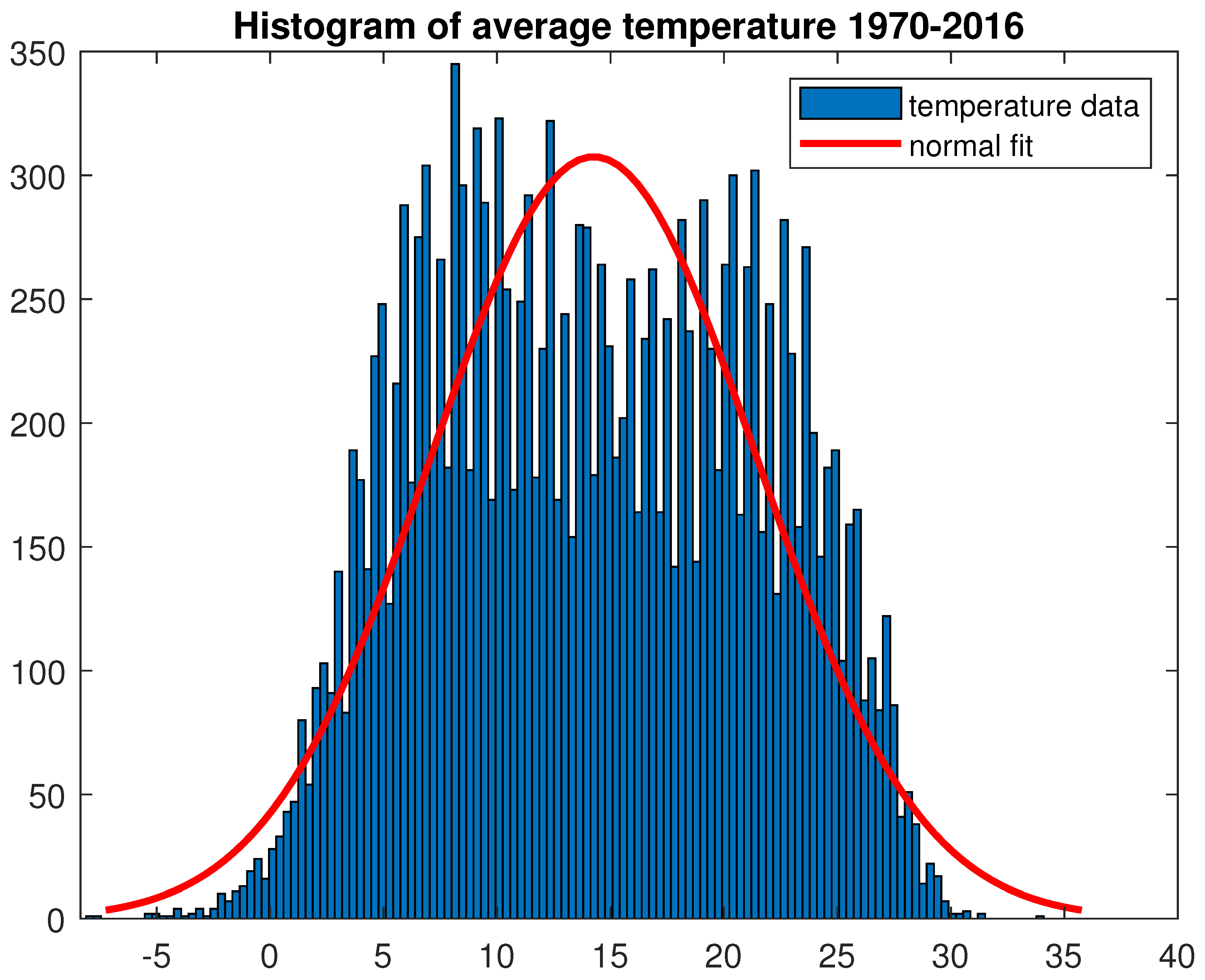
However, while the normal and Student’s-t distributions quite efficiently fit a number of financial time series; this is not the case for most meteorological data (see Figure 2).
As it is well known, historically speaking the first theoretical distribution applied in mathematical finance is the normal one. Empirical investigation has shown that real financial data are characterized almost ubiquitously by extreme events; in fact, large losses occur with a frequency that the normal distribution is unable to predict.
VaR and ES are risk measures developed to hedge such potential losses. Their numerical results depend, of course, on the assumed underlying distribution; for a number of distributions (for instance, Student’s-t) explicit formulae exist.
When dealing with temperatures, at least in the area scrutinized in this article, it occurs that historical distribution is bimodal and with thin tails. This leads to the fact that, in this case, VaR and ES become very conservative and prudent ways of representing risk.
The following analysis shows that meteorological data are usually characterized by ‘thin’, rather than ‘fat’, tails.
To this end, an analysis of the tails of the distribution of observed temperatures has been attempted. As it is known, the normal distribution is thin tailed, which is, its upper tail declines to zero faster than exponentially (Pindyck 2011) and that the exponential distribution, whose probability density function is
f x = λ e λ x if x 0 0 if x < 0 ,
is thin-tailed.
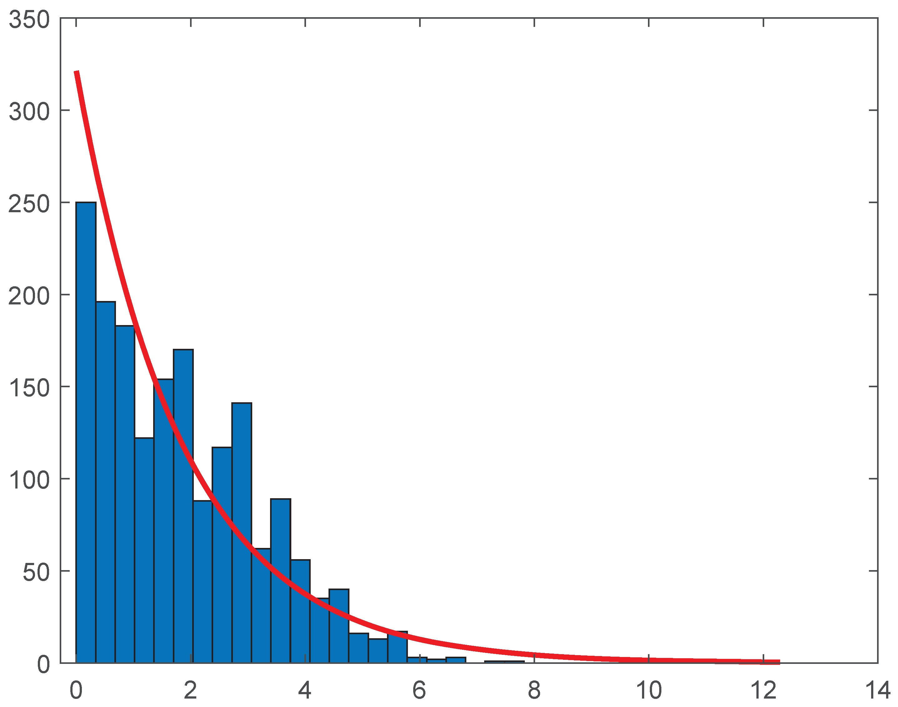
The right tail of such distribution is assumed to be composed of all temperatures that are larger or equal to the 90%th percentile (24 ° C) of the temperature data-set.
In Figure 3, in order to apply the exponential distribution, the 90% percentile has been subtracted to all temperatures. The estimated λ is equal to 1.85997 with 95% confidence interval 1.77605 , 1.95002 .
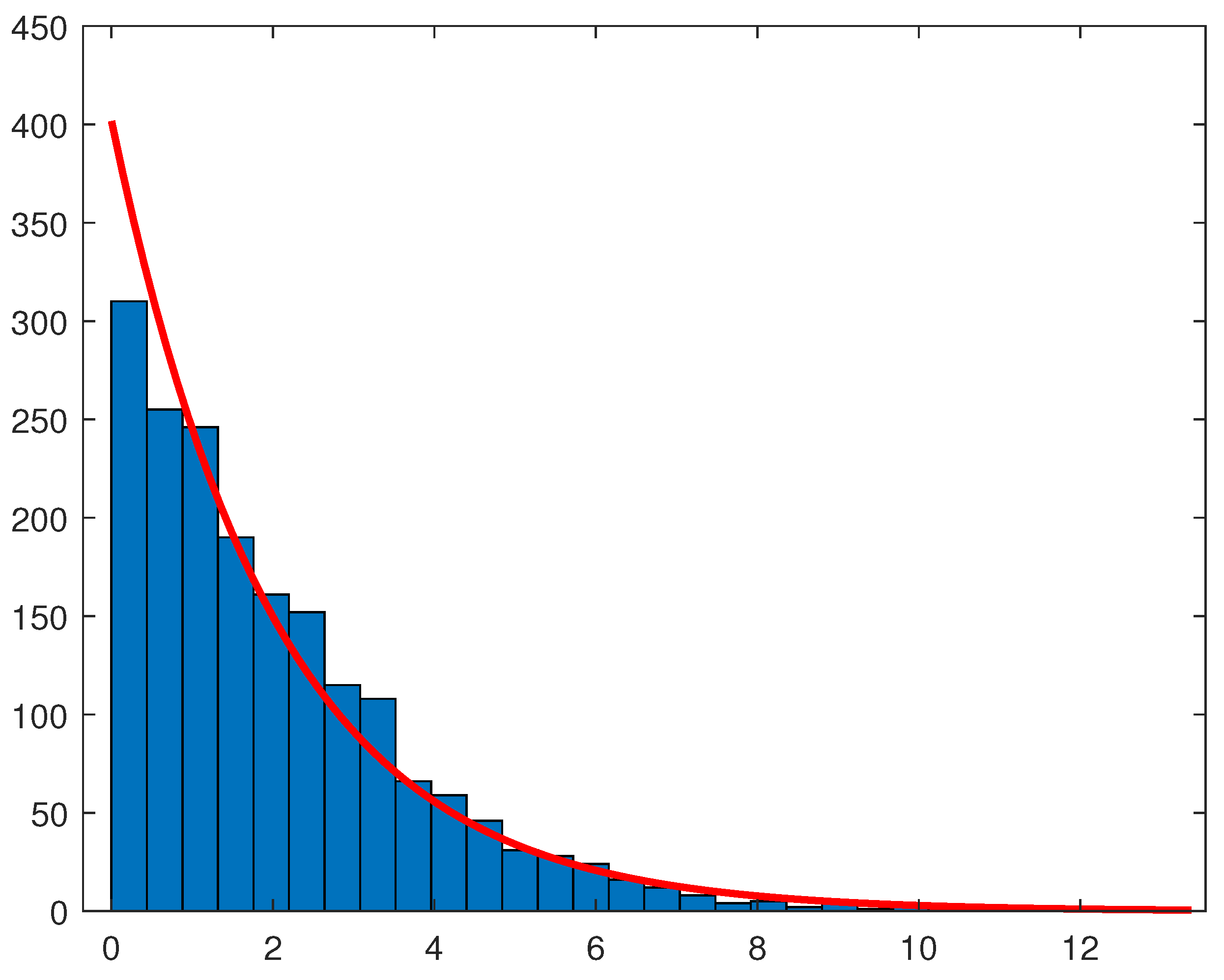
Similarly, the left tail of the distribution under scrutiny is assumed to be composed of all temperatures that are smaller or equal to the 10% percentile ( 5 ° C) of the temperature data-set.
In Figure 4, in order to apply again the exponential distribution, temperatures have been firstly changed in sign (obtaining a right tail). Further, in order to deal with positive numbers, the 10% percentile has been added to all temperatures. The estimated λ is here equal to 2.02396 with 95% confidence interval 1.93481 , 2.11945 .
In conclusion, the temperature distribution shows thin tails. Therefore, the econometric analysis on VaR and ES must keep proper account of this feature. This is achieved by considering the historical and normal methods.
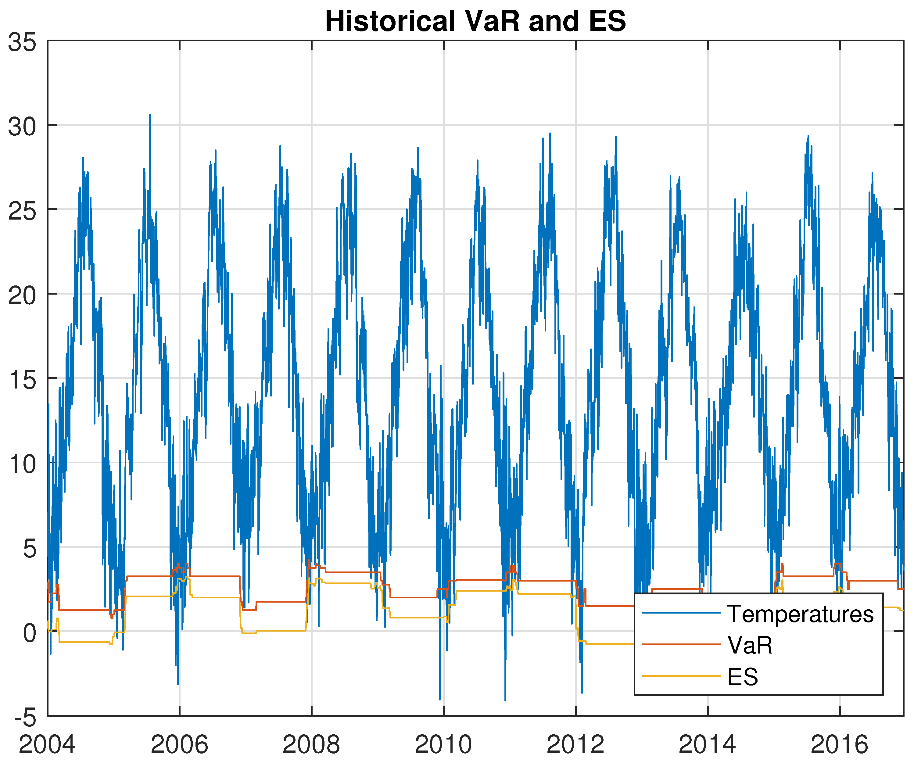
The first method used is the historical one (see Figure 5). The estimation rolling window size is set equal to 365 days, so that a full year of data is used to estimate for both the historical VaR and ES; the sample window runs from the beginning of 2003 through the end of 2016. Following Basel Committee on Banking Supervision (2019), a VaR confidence level of 97.5 % is used.
According to Rockafellar and Uryasev (2002), the historical VaR and ES are computed, as follows:
V a R α = z ( k )
and
E S α = ( k α · N ) z ( k ) + i = k + 1 N z ( i ) N ( 1 α ) if   k < N z ( k ) if   k N
where k = floor α · N , N is the length of the historical data under study, while z is the vector containing all sorted historical data.
Figure 5 shows that the historical simulation curve has a piece-wise constant profile. The reason for this is that quantiles do not change for several days until extreme events occur. Thus, the historical simulation method is slow to react to changes in volatility.
Another estimation method uses parametric models (McNeil et al. 2005); this approach requires computing the volatility of daily average temperatures.
Given this volatility, VaR and ES can be analytically computed assuming that temperatures follow a normal distribution with mean μ and variance σ 2 :
VaR α = μ + σ Φ 1 ( α )
and
ES α = μ + σ ϕ ( Φ 1 ( α ) ) 1 α
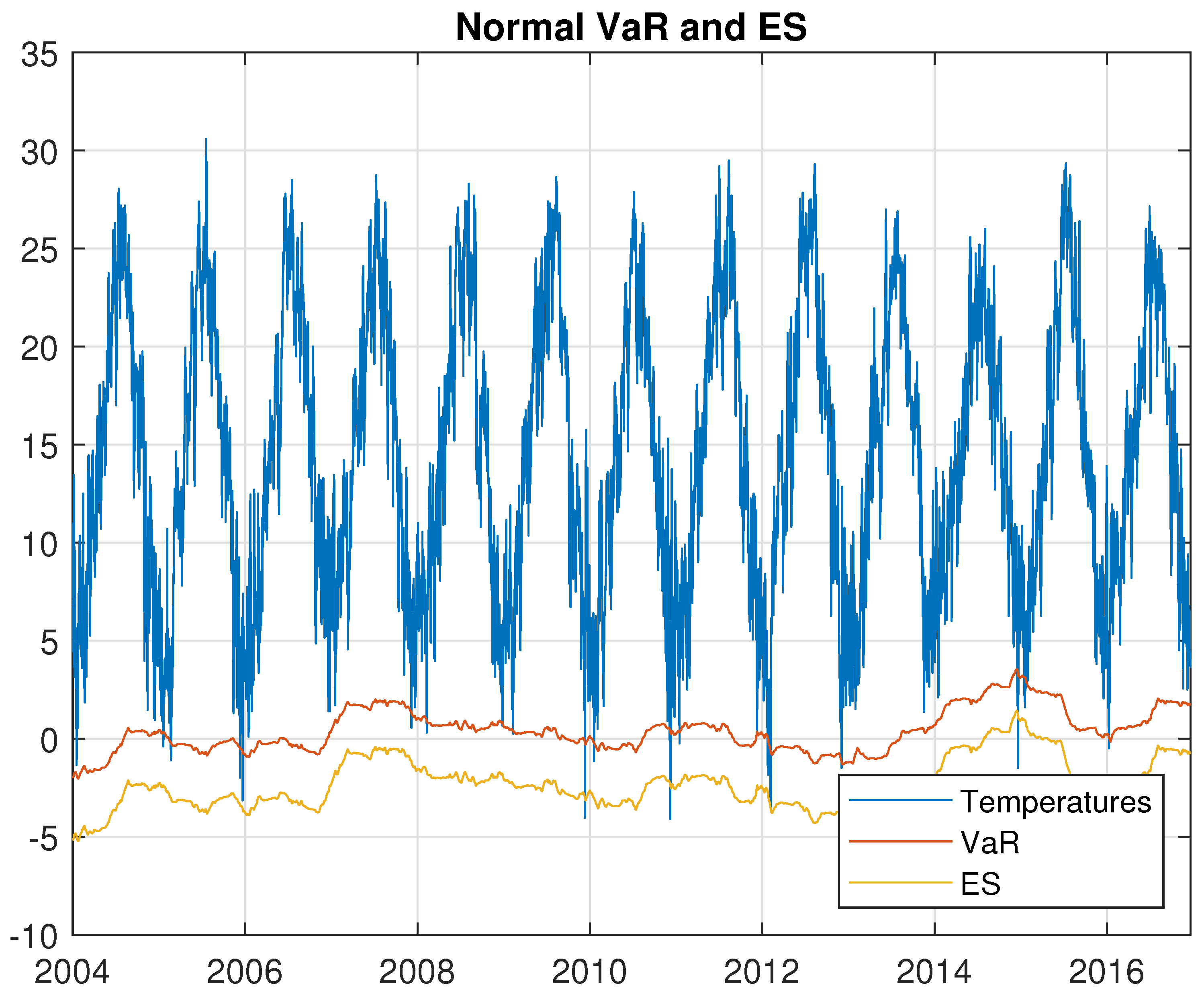
where ϕ and Φ denote density of standard normal distribution and cumulative standard normal distribution, respectively. Φ 1 ( α ) is the α -quantile of Φ . A non-zero mean is assumed and it is estimated as a sum of all yearly means. For the normal distribution, the estimated volatility is directly used to obtain the VaR and ES (see Figure 6).
The data-set under scrutiny has a kurtosis far away from 3, as can be seen from Table 1. To properly test this claim, Table 2 carries the results for two tests for normality of data:
The null hypothesis (data are normally distributed) is rejected by both of them.
To tackle this issue, a more flexible theoretical distribution can be applied. The key point here is to choose a distribution that could somehow be compatible with observed data. A plausible choice is the Student’s-t one. In fact, denoting with ν the number of its degrees of freedom, its skewness is 0 for ν > 3 , while its kurtosis is 6 / ν 4 for ν > 4 , a number compatible with the kurtosis observed (see Table 1).
VaR and ES Formulas for a Student’s-t with ν degrees of freedom T t ( ν , μ , σ 2 ) distribution are
V a R α = μ + σ t ν 1 ( α )
and
E S α = μ + σ g ν ( t ν 1 ( α ) ) 1 α · ( ν + ( t ν 1 ( α ) ) 2 ) ν 1
where t ν is the standard t-distribution c.d.f, t ν 1 is the standard t-distribution quantile and g ν is the standard t-distribution p.d.f.
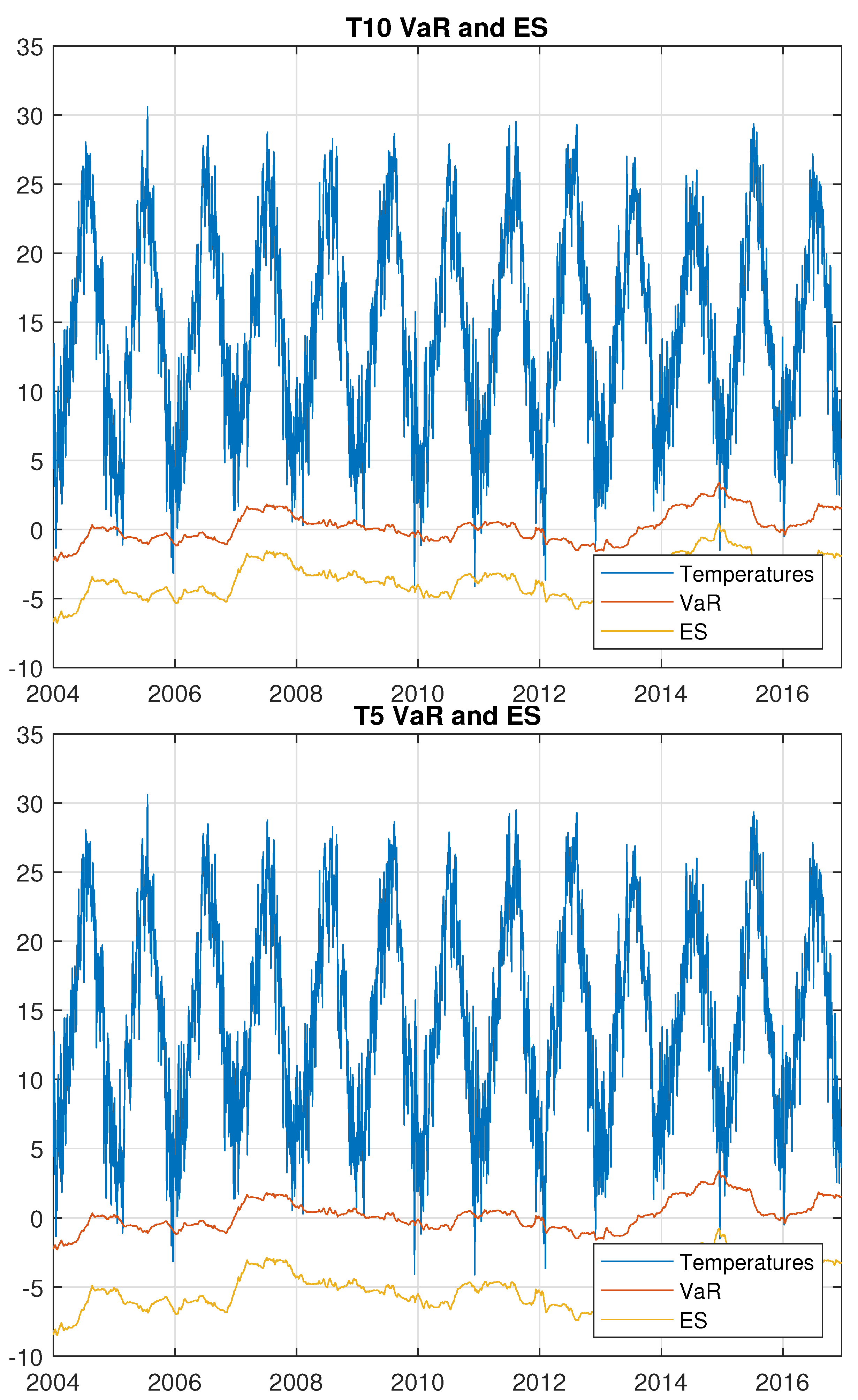
Figure 7 shows the daily temperatures, VaR and ES estimated values with Student’s-t distribution with 10 and 5 degrees of freedom.
No theoretical model can fully catch reality, as is almost always the case. Still, financial literature has deeply analyzed the results obtained by theoretical models applied to real data. On top of this, closed formulas for VaR and ES, for the distributions used in this section, exist. Looking at data under scrutiny, it results that temperatures, at least in this case, have thin tails. Financial agents are, instead, worried about fat fails. This explains why the normal distribution performs better, when compared to the Student’s-t distribution, with the latter being characterized by fatter tails. This observation leads to the idea, to be developed in a subsequent paper, to apply theoretical distributions with thinner tails when compared to the normal distribution ones.
A back-test on ES, which is based on available data, is in Appendix B. Its main result is that the Historical and Normal models perform better and, therefore, will be used in what follows.
Of course, the fact that Arezzo’s temperatures show thin tails could be the result of the fact that Tuscany is located in a very favorable area, meteorologically speaking.
As the aim of the paper is to present a novel approach in pricing weather derivatives by means of VaR and ES, its findings has to be standard and consistent. This leads to the claim that what has been presented here could be possibly used everywhere, regardless of the behavior of the observed meteorological data.
The historical method, of course, does not assume any underlying distribution. On the other hand, as said, the normal method, assuming tails fatter than the observed ones, will give results that are more conservative than taking a better fitting distribution. The claim is that the normal method is the best financial compromise in choosing an underlying distribution, according to the universal standards, without leaving the freedom of applying different methods for finding VaR and ES. In any case, the final results in pricing and hedging are found to be very similar using the historical or the normal method.
4. Temperature-Based Model

To model the temperature dynamics, a time series decomposition approach proposed by Benth and Saltyte-Benth (2013). Temperature T ( t ) is decomposed into a mean component μ ( t ) , which models the trend, and a residual component ϵ ( t ) that models the fluctuations around a trend over time. The temporal decomposition of T ( t ) can be written as:
T ( t ) = μ ( t ) + ϵ ( t )
where μ ( t ) is a deterministic function over time defined as:
μ ( t ) = θ ( t ) + i = 1 p α i ( T ( t i ) θ ( t i ) )
where α i are the parameters of an AR ( p ) process, θ ( t ) is the (linear) trend, and seasonality in terms of the sine and cosine functions in T ( t ) expressed is as follows:
θ ( t ) = a 0 + a 1 t + a 2 cos 2 π t 365 + a 3 sin 2 π t 365 .
The part containing trigonometric functions explains the seasonal variations in temperature. Variable ϵ ( t ) represents residuals at time t in the form:
ϵ ( t ) = σ ( t ) γ ( t )
where σ ( t ) is a (possibly time–dependent) volatility function, γ ( t ) is a zero-mean temporally independent Gaussian random process with standard deviation that is equal to one, and σ ( t ) is a (possibly time–dependent) volatility function given by a truncated Fourier series as follows:
σ 2 ( t ) = b 0 + l = 1 4 b 1 l cos 2 π t 365 + b 1 l + 1 sin 2 π t 365 .
In order to predict average temperature for 2017, the dynamics of ϵ ( t ) is now to be found. To achieve this, parameters for the volatility function σ ( t ) , expressed using a Fourier series of order 2 and applying the standard OLS method, are determined.
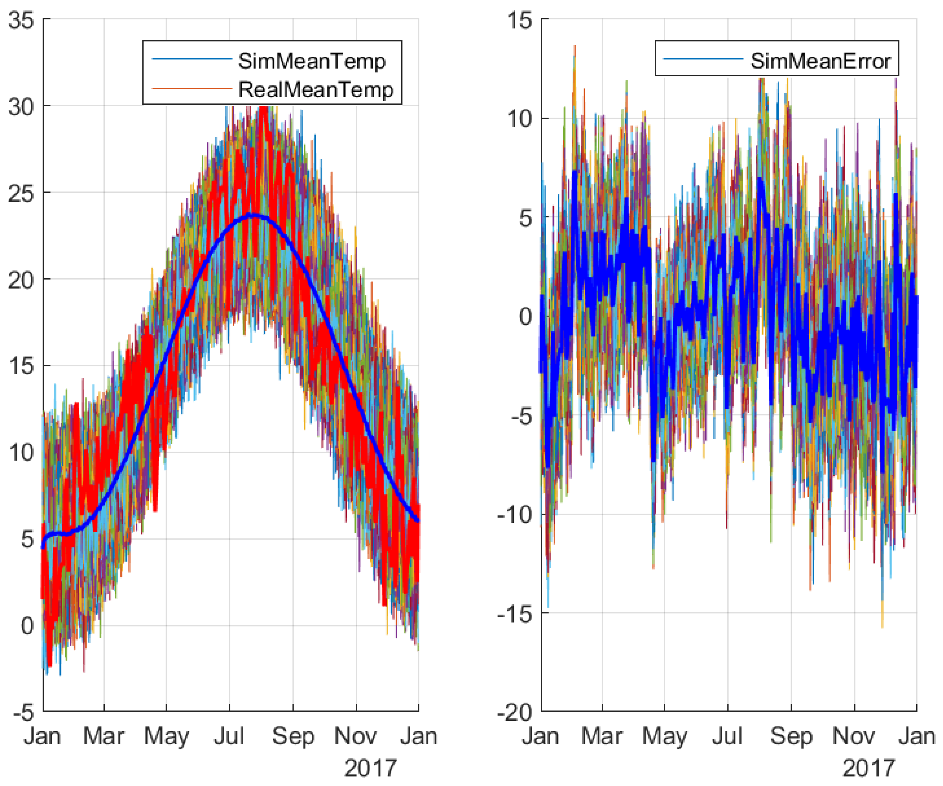
The next step is to simulate 1000 trajectories for γ ( t ) ; this leads to obtaining 1000 trajectories for average temperatures. The lhs of Figure 8 shows such trajectories and how the observed average temperatures (red curve) differ from the simulated average temperatures (blue curve). In the rhs of the same Figure 8, forecast errors for 1000 simulated trajectories with respect to average temperatures of 2017 are displayed.
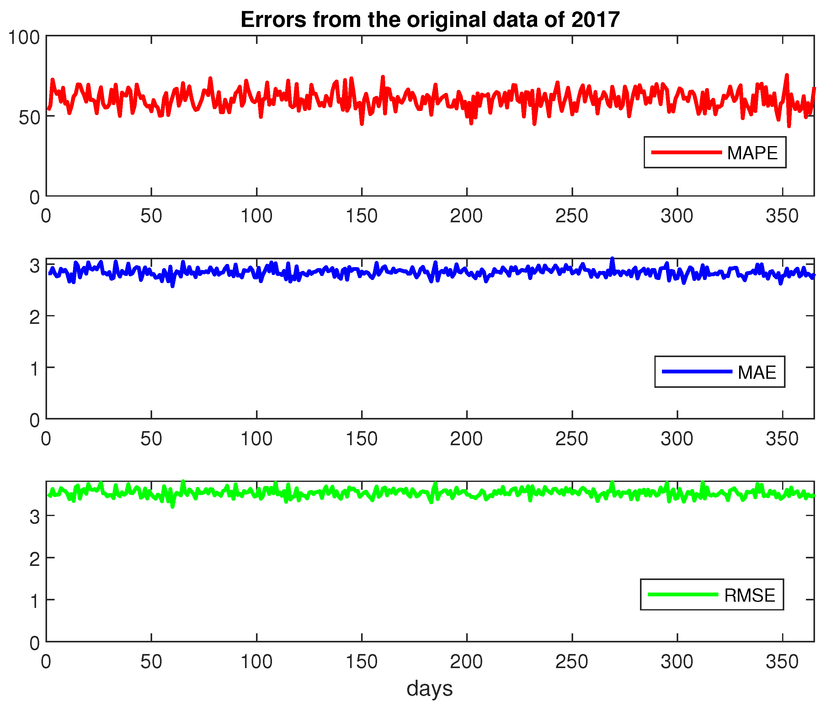
For a more detailed analysis of errors due to simulation, the mean absolute percentage error (MAPE), mean absolute error (MAE), and root mean square error (RMSE) discrepancies of simulated data from the observed average 2017 temperatures have been computed and represented in Figure 9.
These data represent the errors that result when simulated data are compared with the observed 2017 data. In order to at least partially reduce errors displayed above, a ‘removing outliers’ approach will be performed in the next section.

5. Worst Case Approach Based on VaR and ES

In order to reduce uncertainty when calculating WD prices, the method proposed by Benth et al. (2019) is now applied. This is done inside a Monte Carlo framework, in which values for the stochastic component of the temperature model given in (5) are simulated.
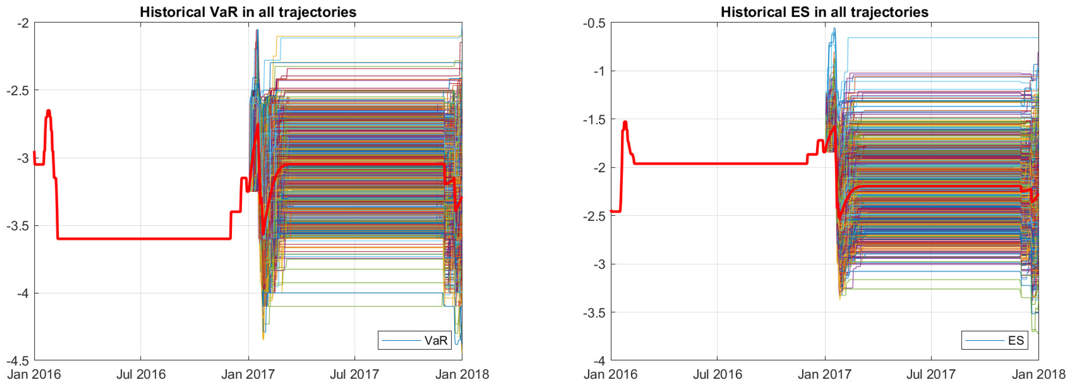
At first, VaR and ES for all trajectories of volatility for year 2017 are computed. Figure 10 shows the VaR and ES obtained by applying the historical method (see Section 3).
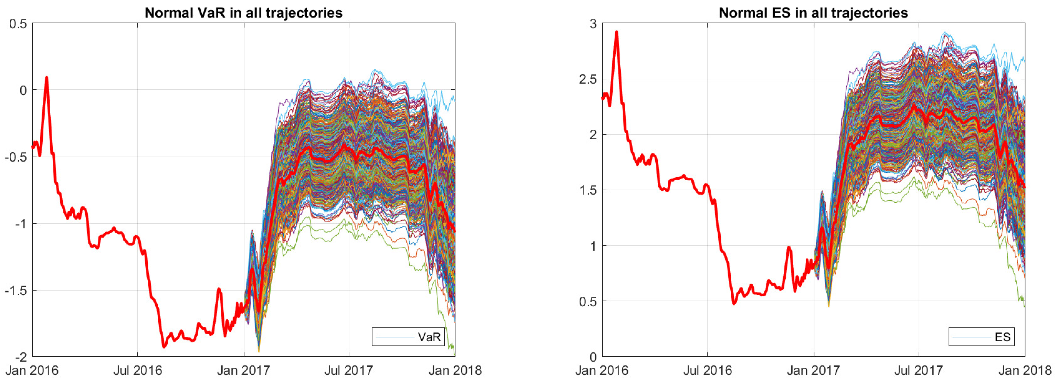
Figure 11 shows VaR and ES obtained by applying the normal method; red curves identify the average of VaR and ES from all of the simulated trajectories.
This being done, applying the worst case approach that is based on VaR and ES removes outliers/worst scenarios that, if not expunged, affect prices of weather derivatives and lead to an increased uncertainty. The elimination of extreme tails approach is based on a η = 2.5 % level.
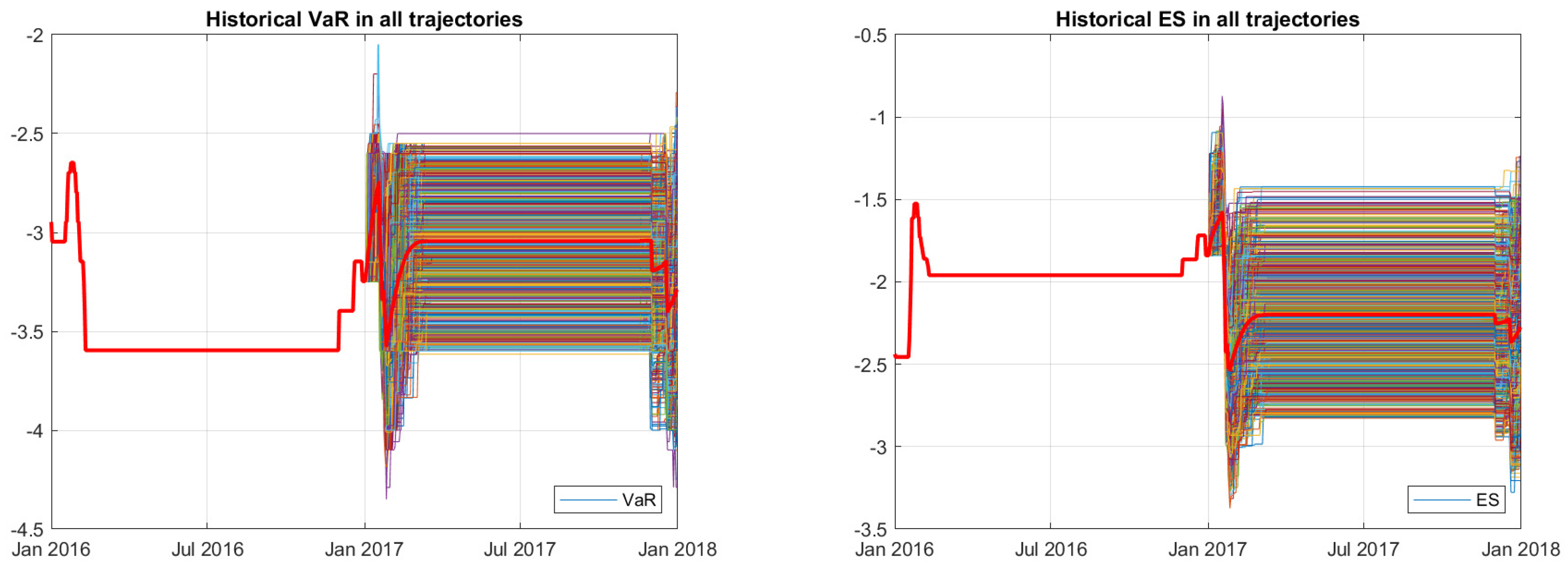
Figure 12 shows VaR and ES after having removed extreme tails by applying the historical method; red curves identify the averages of VaR and ES from the remaining simulated trajectories.
Figure 13 shows VaR and ES after having removed extreme tails by applying the normal method; red curves identify the averages of VaR and ES from the remaining simulated trajectories.
By comparing Figure 12 and Figure 13 with Figure 10 and Figure 11, having removed outliers, the trajectories show a more compact behavior.
In the next section, pricing of pure financial derivatives has been computed removing (Table 3) or not removing (Table 4) extreme tails.

6. Pricing a Temperature-Based Weather Derivative

In this section, the pricing of HDD and CDD (both without and with risk loadings), computed for each month in 2017, are displayed. The temperatures for 2017 have been simulated as said before, while VaR/ES percentiles thresholds have been set equal to 5 % for HDD and 95 % for CDD.
Table 3 encompasses the ‘pure’ financial values of HDD and CDD computed according to formulae (1) and (2) and including tail values discussed above. Table 4 displays the same computations having, instead, removed tail values. The cut-off for considering a value an outlier has been set as equal to 2.5 % .
A comparison between Table 3 and Table 4 shows how the financial prices are not affected by the removal of extreme values. For this reason, and for sake of compactness, the rest of this numerical analysis is going to be performed when considering all values.
To depart from standard actuarial techniques, risk loadings are determined here as a fraction α of the 100 · 1 α percentile of the pay-off distribution of the derivative. Such values are obtained considering the historical temperature time series from 1970 to 2016. As a first step, temperatures are subdivided month by month. Out of these, for each of the twelve sub-sets the 100 · 1 α percentile is determined. Finally, these values become the threshold used to compute the historical pay-off distributions of either HDD and CDD. The complete graphical behavior of these thresholds is depicted above in Figure 1.
By looking at Table 3 and Table 5, it is evident that, as HDD thresholds are lower when ES is applied instead of VaR, prices in the left part of column 2 are lower than those in the right part. A similar but opposite reasoning holds for CDD: here, thresholds are larger for ES rather than VaR so that prices in left part of column 3 are greater then corresponding prices in the right part.
Some descriptive statistics of option values treated in this section can be found in Appendix C.

7. Hedging Strategies with Hybrid Instruments Based on Value-at-Risk and Expected Shortfall

Consider a farmer who needs to hedge against negative weather events in the Arezzo’s area by means of some tailor-made derivative contract.
According to computation that was performed above, the temperature risk for each month in 2017 can be hedged by means of either an HDD or CDD with monthly maturity.
In Benth and Saltyte-Benth (2013), it is stated that Chicago Mercantile Exchange (CME) offers HDD contracts from November to June, while CDD and CAT contracts are offered from May to September. This leads to the conclusion that, when considering WD, some months (i.e., summer and winter seasons) are more relevant than others.
When comparing final prices of these derivatives (see Table 5) with their actual 2017 daily pay-off obtained by using observed data leads to Table 6, where only winter and summer data are reported.
Aside monthly contracts, in order to test if the ES’s diversification property holds in this context, the analysis has been extended to seasonal contracts.
For this reason, two seasonal contracts, the first encompassing the winter period ranging from January to March 2017, the second the summer one (June to August 2017) have been priced with the same methodology applied for monthly WDs.
Table 7 summarizes the pure financial prices (column 2), the full prices (i.e., adding risk loadings—column 3) and profit and losses (column 4) for HDD in the winter 2017 season.
By looking at Table 7, it is evident, in terms of P/L, that a seasonal HDD contract leads to a profit for the insured farmer. Such profit would have turned into a loss in the case that the farmer had bought monthly contracts.
A somehow less clear-cut result occurs for the summer season (see Table 8), where CDD contracts are used. Final column in Table 8 shows that P/L for contracts priced while using VaR as a threshold is larger when considering a three-month duration derivative instead of three monthly CDDs. The opposite results, still leading, though, to a profit, occurs when ES is used.
To end this section, there is no need to say that some variables chosen in the above analysis, such as, for instance, tick sizes and contract maturities, can be chosen, so to match a large number of needs an agent might require to manage weather-related business risks. Insurance companies can, on their side, perform some fine tuning with respect to some quantities that are involved in WD so to avoid facing losses on their side, as displayed in Table 7 and Table 8.
Further, according at least to data that were exploited in this article, the Expected Shortfall shows to maintain, even if not fully, its diversification property. Nevertheless, it has been numerically assessed that seasonal WD derivatives lead to better profit and loss results when compared with monthly contracts written on the same period.

8. Conclusions

This article has presented a way to hedge temperature risk exploiting weather derivatives contracts. This has been achieved when considering ‘tail events’ and the standard financial approach to tackle them: namely, Value-at-Risk and Expected Shortfall.
Using as a starting point historical time series for a very specific area, an ‘hybrid’ contract, composed of a Weather Derivative whose price also encompasses a risk loading, has been evaluated. The aim of this choice is to combine the efficient pricing of a derivative with the gains that are required by an insurer to carry a specific risk.
Pay-offs have been determined by means of a stochastic simulation technique and compared with those that were obtained observing 2017 temperatures.
According to risk measure theory, proved that Expected Shortfall captures diversification while Value-at-Risk does not, the numerical results presented above show that it is more convenient to enter a single contract that covers more months rather than monthly contracts spanned on the same period.
Research performed in this paper can be extended in a number of directions. As meteorological data are easily accessible, a possible extension might encompass different sites, letting for more sources of randomness to be explored. Another path is evaluating more complex derivatives instead of standard options. Beside this, the fact that temperatures present thin tails is an interesting, as well as a non-standard financial issue, research topic. Finally, a full comparison between hybrid and tailored-made Weather Derivatives and the financial contracts periodically issued on some regulated market, such as the Chicago Mercantile Exchange, might further shed some more light on this specific field.

Author Contributions

All authors have contributed equally to this work. All authors have read and agreed to the published version of the manuscript.

Funding

This research received no external funding.

Acknowledgments

The authors of this paper gratefully thank the staff at the Servizio Idrologico Regionale della Regione Toscana (SIR) for its excellent management of data source and the referees whose precious reports helped to substantially improve and ameliorate this paper.

Conflicts of Interest

The authors declare no conflict of interest.

Appendix A

Two of the most common quantile-based risk measures are Value-at-Risk (VaR) and Expected Shortfall (ES).
In general terms, let X Ω be a random variable depicting the future outcome in T > 0 of a risk. In the ADEH framework, a risk manager is assumed to be always capable of distinguishing between acceptable and non acceptable risks.
Let A ( A C = Ω A ) be the set containing all acceptable (non acceptable) risks. In order for the theory to be consistent, these sets must obey some “common sense” assumptions.
If Y A C , a risk measure is some function ρ : Ω R defined as
inf β β v : Y + β A
where β is a positive amount of money while v is the risk-less discount factor in 0 ; T .
A risk measure is, then, the smallest amount of money β to be added to a non acceptable random variable Y that makes it, as some future epoch, Y + β an acceptable one.
Let
F X x = P X x x R
be the distribution function for a monetary-measured risk X and consider α , 0 < α < 1 , a probability level.
  • the Value-at-Risk (VaR) for a risk X with 1 α confidence level is defined as
    VaR α X = inf z F X z > α ,
    If X A C X A , then VaR α X > 0 VaR α X < 0
  • the Expected Shortfall (ES) for a risk X with 1 α confidence level is expressed as
    ES α X = E X | X VaR α X
Even if such tail-based risk measures look appropriate in handling WD features, ADEH’s work determines a fundamental result in risk management: some measures are unable to capture fully capture risks.
VaR, for instance is not a sub-additive measure. Let X , Y Ω be two risks.
It can be shown that
VaR α X + VaR α Y VaR α X + Y
a feature that defies the notion of diversification: when analyzing two, or more, risks together, VaR might suggests not tohedge by means of a portfolio of random variables but to invest all the money into a single asset.
Otherwise said, the right hand side of inequality (A1) reports that risks X and Y , measured separately, are not as risky as the same risks included in a portfolio.
ES is instead sub-additive:
ES α X + ES α Y ES α X + Y .
A complete discussion of risk measures can be found in Artzner et al. (1999); Meucci (2009).

Appendix B

This section presents the ES back-test in order to assess the performance of the non-parametric and parametric models studied in the previous section. The ES back-test uses the unconditional test statistics proposed by Acerbi and Szekely (2014), given by
Z u n c = 1 N p VaR t = 1 N T t I t E S t + 1
where N is the number of observations, T t is the temperature for period t, p VaR is the probability of VaR failure defined as 1 VaR level, I t is the VaR failure indicator on period t with a value of 1 if T t < VaR t , and 0 otherwise and E S t is the estimated expected shortfall for period t expressed as follows:
E S t = E t T t I t p VaR ,
where operator E t stands for the expected value conditioned to information available up to time t.
The expected value for this test statistics is 0; it should be negative when there is evidence of risk under-estimation. To determine how negative this estimate should be for the model to be rejected, some critical values are needed. These, of course, require some distributional assumptions on the observed variable T t .
The unconditional test statistics turns out to be stable across a range of distributional assumptions for T t , from thin-tailed distributions through the normal one and up to heavy-tailed distributions such as Student’s t with a few degrees of freedom. Only very heavy-tailed Student’s t-distributions lead to more noticeable differences in the critical values (see Acerbi and Szekely (2014)). The ES back-test takes advantage of the stability of the critical values of the unconditional test statistic and uses tables of pre-computed critical values to run ES back tests. The ES back-test has two sets of critical-value tables. The first set of critical values assumes that the temperature outcomes T t follow a standard normal distribution; this is the unconditional normal test. The second set of critical values uses the heaviest possible tails, it assumes that the temperature outcomes T t follow a t distribution with ν = 3 degrees of freedom; this is the unconditional t-test.
The unconditional test statistics is sensitive to both the severity of the VaR failures relative to the ES estimate, and also to the number of VaR failures (how many times the VaR is violated, since, whenever losses exceed VaR, a VaR violation occurs).
Expected average ratio is the average ratio of ES to VaR, over the period under scrutiny, with VaR failures while observed average severity ratio is the average ratio of loss to VaR over the periods with VaR failures.
Therefore, a single but very large VaR failure relative to the ES may cause the rejection of a model in a particular time window. A large increase/decrease of temperature on a day when the ES estimate is also large may not impact the test results as much as a large increase/decrease of temperature when the ES is smaller. A model can also be rejected in periods with many VaR failures, even if all the VaR violations are relatively small and only slightly higher than the VaR.
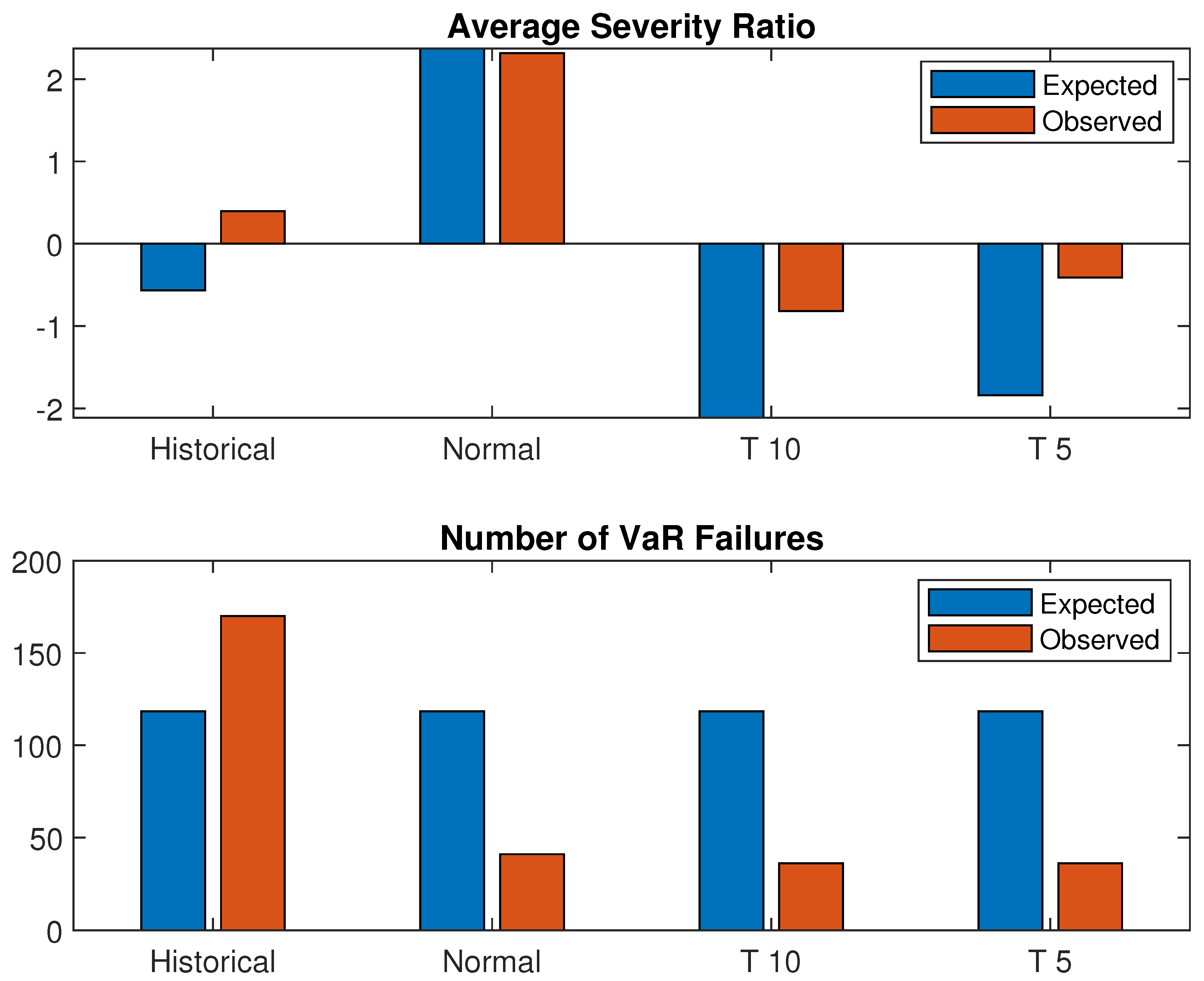
In Figure A1 the observed severity column shows the average ratio of increased/decreased temperature to VaR on periods when the VaR was violated. The expected severity column uses the average ratio of ES to VaR for the VaR violation periods. For the “Historical” and “Normal” models, the observed and expected severities are comparable. However, for the Historical method, the observed number of failures (red bars) is considerably higher than the expected number of failures (blu bars), about 2% higher. Both the “T5” and the “T10” models have observed severities much higher than the expected ones.
Figure A1. Severity of VaR failures relative to the ES estimate and to the number of VaR failures.
Risks 08 00118 g0a1
For the 2004–2016 window, all models pass both tests with a 95 % level.
Even though all models pass both tests, it is clear from Figure A1 that T5 and T10 have a higher average severity ratio and number of VaR failures. To conclude this section, it results that from all the four methods (Historical, Normal, T5 and T10) under study, Historical and Normal VaR and ES are the ones that perform better when applied to the temperature data-set under scrutiny.

Appendix C

The following tables report some descriptive statistics for option data. Table A1 and Table A2 show some descriptive statistics for seasonal HDD and CDD option contracts. Months considered for seasonal HDD are January to June, for seasonal CDD such months are May to September.
Table A1. Descriptive Statistics for seasonal HDDs for the period of time 1970–2016 and 10% percentile threshold.
Temp. ( ° C)MeanVarStd DevMinMaxSkewnessKurtosis
VaR ( K = 4.25 ° C)40.431503.1938.773.25236.653.0513.68
ES ( K = 2.27 ° C)13.06231.4815.21065.861.994.28
Table A2. Descriptive Statistics for seasonal CDDs for the period of time 1970–2016 and 90% percentile threshold.
Temp. ( ° C)MeanVarStd DevMinMaxSkewnessKurtosis
VaR ( K = 26 ° C)19.38316.6117.79083.51.442.53
ES ( K = 20.26 ° C)303.418112.5190.07102.51565.110.270.47
Table A3 and Table A4 show descriptive statistics for June monthly HDD and CDD.
Table A3. Descriptive Statistics for monthly HDDs for the period of time 1970–2016 and 10% percentile threshold.
Temp. ( ° C)MeanVarStd DevMinMaxSkewnessKurtosis
VaR ( K = 16.5 ° C)40.433.4417.464.1801.772.78
ES ( K = 15.24 ° C)1.084.332.0809.042.445.62
Table A4. Descriptive Statistics for monthly CDDs for the period of time 1970–2016 and 90% percentile threshold.
Temp. ( ° C)MeanVarStd DevMinMaxSkewnessKurtosis
VaR ( K = 24.4 ° C)3.9443.476.59027.52.073.64
ES ( K = 19.97 ° C)45.54744.3927.2812.26144.751.392.56

References

  1. Acerbi, Carlo, and Balazs Szekely. 2014. Back-testing expected shortfall. Risk 27: 76–81. [Google Scholar]
  2. Acerbi, Carlo, and Dirk Tasche. 2002. Expected shortfall: A natural coherent alternative to value at risk. Economic Notes 31: 379–88. [Google Scholar] [CrossRef] [Green Version]
  3. Alaton, Peter, Boualem Djehiche, and David Stillberger. 2002. On modelling and pricing weather derivatives. Applied Mathematical Finance 9: 1–20. [Google Scholar] [CrossRef]
  4. Alexandridis, Antonis K., and Achilleas D. Zapranis. 2013. The weather derivatives market. In Weather Derivatives. New York: Springer, pp. 1–20. [Google Scholar]
  5. Artzner, Philippe, Freddy Delbaen, Jean-Marc Eber, and David Heath. 1999. Coherent measures of risk. Mathematical Finance 9: 203–8. [Google Scholar] [CrossRef]
  6. Barger, Norah, and Alan Adkins. 2013. Consultative Document: Fundamental Review of the Trading Book Rules—Further Response. Available online: https://www.gfma.org/wp-content/uploads/0/83/91/161/69270c81-740c-4447-bcdd-5ecbadd0a88a.pdf (accessed on 18 July 2020).
  7. Basel Committee on Banking Supervision. 2019. Minimum Capital Requirements for Market Risk. Available online: https://www.bis.org/bcbs/publ/d457.htm (accessed on 18 July 2020).
  8. Benth, Fred Espen, Gleda Kutrolli, and Silvana Stefani. 2019. Dynamic Probabilistic Forecasting with Uncertainty. Available online: https://papers.ssrn.com/sol3/papers.cfm?abstract_id=3405890 (accessed on 18 July 2020).
  9. Benth, Fred Espen, and Jurate Saltyte-Benth. 2005. Stochastic modeling of temperature variations with a view towards weather derivatives. Applied Mathematical Finance 12: 53–85. [Google Scholar] [CrossRef]
  10. Benth, Fred Espen, and Jurate Saltyte-Benth. 2011. Weather Derivatives and Stochastic Modelling of Temperature. International Journal of Stochastic Analysis. [Google Scholar] [CrossRef]
  11. Benth, Fred Espen, and Jurate Saltyte-Benth. 2013. Modeling and Pricing in Financial Markets for Weather Derivatives. Singapore: World Scientific, vol. 17. [Google Scholar]
  12. Black, Fisher, and Myron Scholes. 1973. The pricing of options and corporate liabilities. Journal of Political Economy 81: 637–54. [Google Scholar] [CrossRef] [Green Version]
  13. Brix, Anders, Stephen Jewson, and Christine Ziehmann. 2005. Weather Derivative Valuation: The Meteorological, Statistical, Financial and Mathematical Foundations. Cambridge: Cambridge University Press. [Google Scholar]
  14. Kelly, David L., Charles D. Kolstad, and Glenn T. Mitchell. 2005. Adjustment costs from environmental change. Journal of Environmental Economics and Management 50: 468–95. [Google Scholar] [CrossRef]
  15. Le Den, Xavier, Matilda Persson, Audrey Benoist, Paul Hudson, Marleen de Ruiter, Lars de Ruig, and Onno Kuik. 2017. Insurance of Weather and Climate-Related Disaster Risk: Inventory and Analysis of Mechanisms to Support Damage Prevention in the EU. Available online: https://op.europa.eu/en/publication-detail/-/publication/4f366956-a19e-11e7-b92d-01aa75ed71a1/language-en (accessed on 18 July 2020).
  16. McNeil, Alexander J., Rüdiger Frey, and Paul Embrechts. 2015. Quantitative Risk Management: Concepts, Techniques and Tools—Revised Edition. Princeton: Princeton University Press. [Google Scholar]
  17. Merton, Robert C. 1973. Theory of rational option pricing. The Bell Journal of Economics and Management Science 4: 141–83. [Google Scholar] [CrossRef] [Green Version]
  18. Meucci, Attilio. 2009. Risk and Asset Allocation. Berlin: Springer. [Google Scholar]
  19. Mills, Evan. 2005. Insurance in a climate of change. Science 309: 1040–44. [Google Scholar] [CrossRef] [PubMed] [Green Version]
  20. Pindyck, Robert S. 2011. Fat tails, thin tails, and climate change policy. Review of Environmental Economics and Policy 5: 258–74. [Google Scholar] [CrossRef]
  21. Rockafellar, Tyrrell R., and Stanislav Uryasev. 2002. Conditional Value-at-Risk for general loss distributions. Journal of Banking and Finance 26: 1443–71. [Google Scholar] [CrossRef]
  22. Saltyte-Benth, Jurate, and Fred Espen Benth. 2012. A critical view on temperature modeling for application in weather derivatives markets. Energy Economics 34: 592–602. [Google Scholar] [CrossRef] [Green Version]
  23. Stefani, Silvana, Enrico Moretto, Matteo Parravicini, Simone Cambiaghi, Adeyemi Sonubi, Gleda Kutrolli, and Vanda Tulli. 2018. Managing adverse temperature conditions through hybrid financial instruments. Journal of Energy Markets 11: 25–41. [Google Scholar]
  24. Taib, Che Mohd Imran Che, and Fred Espen Benth. 2012. Pricing of temperature index insurance. Review of Development Finance 2: 22–31. [Google Scholar] [CrossRef] [Green Version]
  25. Tang, Chun-Hung Hugo, and SooCheong Shawn Jang. 2011. Weather risk management in ski resorts: Financial hedging and geographical diversification. International Journal of Hospitality Management 30: 301–11. [Google Scholar] [CrossRef]
  26. Tang, Chun-Hung Hugo, and SooCheong Shawn Jang. 2012. Hedging Weather Risk in Nature-Based Tourism Business: An Example of Ski Resorts. Journal of Hospitality & Tourism Research 36: 143–63. [Google Scholar]
  27. Wang, Zhiliang, Peng Li, Lingyong Li, Chunyan Huang, and Min Liu. 2015. Modeling and forecasting average temperature for weather derivative pricing. Advances in Meteorology 2015: 1–8. [Google Scholar] [CrossRef]
  28. Zenghelis, Dimitri. 2006. The Stern Review on the Economics of Climate Change. Available online: http://videolectures.net/site/normal_dl/tag=12665/ccog07_zenghelis_tsr_01.pdf (accessed on 18 July 2020).
1.
2.
Figure 1. Thresholds K α VaR and K α ES for heating degree days (HDD) and cooling degree days (CDD) for different confidence levels and in different months (HDD corresponds to percentiles 0% to 50% while CDD corresponds to percentiles 50% to 100%). Note that the abbreviations J 1 , A 1 , J 2 , J 3 , and A 2 are used to identify the months of January, April, June, July, and August, respectively.
Risks 08 00118 g001
Figure 2. Historical distribution for daily temperature, Arezzo, 1970–2016.
Risks 08 00118 g002
Figure 3. Exponential fit of temperature distribution—tail beyond 90% percentile.
Risks 08 00118 g003
Figure 4. Exponential fit of temperature distribution—tail below 10% percentile.
Risks 08 00118 g004
Figure 5. The daily average temperature, Value-at-Risk (VaR), and Expected Shortfall (ES) estimated with the historical method.
Risks 08 00118 g005
Figure 6. The daily average temperature, VaR, and ES estimated with the normal method.
Risks 08 00118 g006
Figure 7. Daily average temperature, VaR and ES estimated with the T10 and T5 methods.
Risks 08 00118 g007
Figure 8. Simulated mean temperature and errors for each trajectory for year 2017.
Risks 08 00118 g008
Figure 9. Daily errors of simulated data when compared to observed 2017 temperatures (mean absolute percentage error (MAPE), mean absolute error (MAE), and root mean square error (RMSE)).
Risks 08 00118 g009
Figure 10. Simulated VaR and ES for 2017 obtained by means of 1000 trajectories using the historical method.
Risks 08 00118 g010
Figure 11. Simulated VaR and ES for 2017 applying in 1000 different trajectories using the normal method.
Risks 08 00118 g011
Figure 12. Simulated VaR and ES for 2017 upon removing extreme tails using historical method.
Risks 08 00118 g012
Figure 13. The simulated VaR and ES for 2017 after removing extreme tails using normal method.
Risks 08 00118 g013
Table 1. Descriptive Statistics of the daily average temperature in Arezzo (Tuscany) 1970–2016.
MeanVarStd DevMinMaxSkewnessKurtosis
Temp. ( ° C) 14.26 51.34 7.17 8.1 34 0.028 2.01
Table 2. Normality tests of temperature data in Arezzo (Tuscany), 1970–2016.
Jarque-BeraLillefors (Kolmogorov-Smirnov)
Statistic value 693.99 0.0564
p-value 0.001 0.001
Table 3. Pure financial derivative values for heating degree days (HDD) and CDD computed from data simulated for 2017—thresholds 5 % for HDD and 95 % for CDD—tick size λ = 20 EUR—tail values have not been removed.
MonthHDD (VaR/ES)CDD (VaR/ES)
January 48.92 / 19.15 EUR 55.09 / 846.03 EUR
February 35.49 / 11.84 EUR 116.39 / 805.06 EUR
March 50.65 / 17.18 EUR 43.59 / 958.18 EUR
April 36.43 / 12.71 EUR 83.09 / 845.55 EUR
May 33.81 / 11.39 EUR 46.08 / 849.19 EUR
June 25.90 / 11.66 EUR 73.05 / 833.31 EUR
July 35.28 / 10.16 EUR 34.13 / 741.01 EUR
August 38.17 / 12.88 EUR 30.76 / 816.59 EUR
September 34.63 / 11.83 EUR 69.72 / 834.55 EUR
October 45.56 / 14.59 EUR 28.51 / 938.44 EUR
November 33.52 / 10.98 EUR 79.63 / 954.93 EUR
December 51.28 / 17.91 EUR 38.86 / 924.04 EUR
Table 4. Pure financial derivative values for HDD and CDD computed from data simulated for 2017—thresholds 5 % for HDD and 95 % for CDD—tick size λ = 20 EUR—tail values have been removed.
MonthHDD (VaR/ES)CDD (VaR/ES)
January 48.90 / 19.14 EUR 55.08 / 846.02 EUR
February 35.48 / 11.83 EUR 116.38 / 805.05 EUR
March 50.64 / 17.17 EUR 43.59 / 958.18 EUR
April 36.42 / 12.70 EUR 83.07 / 845.54 EUR
May 33.80 / 11.38 EUR 46.09 / 849.18 EUR
June 25.90 / 11.66 EUR 73.04 / 833.30 EUR
July 35.27 / 10.15 EUR 34.12 / 741.00 EUR
August 38.16 / 12.87 EUR 30.75 / 816.58 EUR
September 34.62 / 11.82 EUR 69.70 / 834.53 EUR
October 45.55 / 14.58 EUR 28.50 / 938.43 EUR
November 33.51 / 10.97 EUR 79.62 / 954.92 EUR
December 51.27 / 17.90 EUR 38.85 / 924.03 EUR
Table 5. Final prices (i.e., financial value + risk loadings) for HDD and CDD—simulations for 2017—tick size λ = 20 Euro—thresholds 5 % for HDD and 95 % for CDD—tail values have not been removed.
MonthsHDD (VaR/ES)CDD (VaR/ES)
January 61.09 / 24.09 EUR 65.08 / 926.09 EUR
February 41.95 / 16.70 EUR 170.62 / 889.76 EUR
March 67.43 / 25.57 EUR 57.31 / 1084.86 EUR
April 46.99 / 17.57 EUR 96.4 / 928.79 EUR
May 41.03 / 13.98 EUR 52.64 / 935.06 EUR
June 33.39 / 15.85 EUR 84.54 / 920.02 EUR
July 44.59 / 13.76 EUR 40.28 / 822.81 EUR
August 47.43 / 18.22 EUR 38.48 / 922.24 EUR
September 44.32 / 14.27 EUR 79.82 / 929.98 EUR
October 56.18 / 18.39 EUR 36.13 / 1048.33 EUR
November 43.19 / 14.08 EUR 92.49 / 1029.81 EUR
December 63.59 / 22.69 EUR 49.41 / 1006.49 EUR
Table 6. HDD and CDD Profit/Losses for 2017—Prices in Table 5 have been compared with actual 2017 pay-offs.
MonthsHDD (VaR/ES)CDD (VaR/ES)
January 85.51 / 20.92 EUR−65.08/−744.92 EUR
February−41.95/−16.70 EUR−120.62/354.61 EUR
March−67.43/−25.56 EUR−12.71/408.03 EUR
June−33.39/−15.85 EUR−52.54/828.07 EUR
July−44.59/−13.76 EUR−21.28/188.90 EUR
August−38.43/−18.22 EUR 147.52 / 816.34 EUR
Table 7. Comparison between HDDs pure financial prices, financial prices + risk loadings (RL) and Profit and Loss (P/L) − winter season 2017.
MonthsPure Fin. Prices (VaR/ES)Fin. Prices + RL (VaR/ES)P/L (VaR/ES)
Winter season 138.12 / 48.92 EUR 162.64 / 58.4 EUR 111.36 / 28.61 EUR
Jan-Feb-Mar 135.06 / 48.17 EUR 170.47 / 66.36 EUR−23.87/−21.34 EUR
Table 8. Comparison between CDDs pure financial prices, financial prices + RL and P/L − summer season 2017.
MonthsPure Fin. Prices (VaR/ES)Fin. Prices + RL (VaR/ES)P/L (VaR/ES)
Summer season 88.60 / 2638.38 EUR 107.97 / 2877.86 EUR 242.03 / 1754.69 EUR
Jun-Jul-Aug 137.94 / 2390.91 EUR 163.30 / 2665.07 EUR 73.70 / 1833.31 EUR
Publisher’s Note: MDPI stays neutral with regard to jurisdictional claims in published maps and institutional affiliations.