Good-Deal Bounds for Option Prices under Value-at-Risk and Expected Shortfall Constraints

Abstract

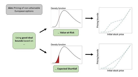
In this paper, we deal with the pricing of European options in an incomplete market. We use the common risk measures Value-at-Risk and Expected Shortfall to define good-deals on a financial market with log-normally distributed rate of returns. We show that the pricing bounds obtained from the Value-at-Risk admit a non-smooth behavior under parameter changes. Additionally, we find situations in which the seller’s bound for a call option is smaller than the buyer’s bound. We identify the missing convexity of the Value-at-Risk as main reason for this behavior. Due to the strong connection between good-deal bounds and the theory of risk measures, we further obtain new insights in the finiteness and the continuity of risk measures based on multiple eligible assets in our setting.

1. Introduction

Pricing in incomplete financial markets is a demanding task for which various approaches are considered in the finance literature. On the one hand, no arbitrage pricing theory leads to wide price ranges. On the other hand, equilibrium theory could give unique prices, but these are not very robust with respect to (w.r.t.) model parameter changes. The theory of good-deal bounds is a compromise between these two concepts. Essentially, good-deals provide portfolios, which are acceptable in terms of the risk measure under consideration, but which have price zero. So, a good-deal bound not only excludes prices that lead to arbitrage opportunities, but also good-deals and thus prices that are viewed as too favorable for one of the market participants.

The important point is the way of quantifying a good-deal. The seminal paper of Cochrane and Saa-Requejo (2000) uses Sharpe-ratios to define good-deals. This approach is extended in Černý (2003) and Björk and Slinko (2006). Bernardo and Ledoit (2000) look at the gain-loss ratio. Another approach are test measures and floors, see for example, Carr et al. (2001). This idea is extended to a dynamic framework in Larsen et al. (2005). Černý and Hodges (2002) put together all these ideas and present a unifying theory for good-deal bounds. They also draw parallels to the classical arbitrage pricing theory. Arai (2011) uses risk measures based on shortfall risk to determine good-deal bounds. The strong connection between good-deal bounds and risk measures is presented for the first time in Jaschke and Küchler (2001). The extension of their results to a non-coherent set of good-deals can be found in Staum (2004). Different representation results for convex risk measures in a pricing setup are given in Arai and Fukasawa (2014) and Farkas et al. (2015).

To the best of our knowledge, there is no comprehensive analysis of good-deal bounds characterized by acceptance sets based on Value-at-Risk and on Expected Shortfall. We would like to fill this gap in a special but standard market setting. Therefore, we use the concept of risk measures based on multiple eligible assets as for example, given in Scandolo (2004), Artzner et al. (2009) and Farkas et al. (2015). They are an extension of risk measures based on a single eligible asset, see Artzner et al. (1999). Inspired by Cochrane and Saa-Requejo (2000), our focus lies on the pricing of European type options in a Black-Scholes market setup without intermediate trading. The restriction to a one-period market model is justified by the following reasons: First of all, for discrete time models the problem of pricing in an incomplete market is rather the rule than the exception. Second, recent works in the field of risk measures are restricted to such kind of models, see for example, Liebrich and Svindland (2017), Liebrich and Svindland (2019) and Baes et al. (2020).

Our contributions are divided into three main parts, corresponding to Section 3, Section 4 and Section 5. In Section 3 we examine risk measures based on multiple eligible assets. In our one-period market model, we find an equivalent condition to the so-called absence of acceptability arbitrage condition in Artzner et al. (2009). If this condition is fulfilled, the multi-asset risk measure is finite. For the coherent acceptance set based on the Expected Shortfall this is a consequence of the results in Farkas et al. (2015). In Section 3.2 we also use their results to prove lower semicontinuity for the multi-asset risk measure w.r.t. the non-coherent acceptance set based on the Value at Risk. But the results in Farkas et al. (2015) do not apply in our concrete setting for showing that the multi-asset risk measure w.r.t. the Value-at-Risk is finite and not globally upper semicontinuous. We prove this in Proposition 3 and Theorem 2. As a concrete application, we choose an European option payoff as future risky position. For its risk calculation we develop numerical approaches to determine the value and the optimal solution of these risk measures. The benefits of fast algorithms is for example, pointed out in (Björk and Slinko 2006, Section 5): “[...] the problem of numerically determining good-deal bounds is relatively complex in terms of CPU time, so there is a very clear need to develop fast, approximative good-deal pricing algorithms”.

In Section 4 we find new relations between the absence of acceptability arbitrage condition and the absence of good-deals of the first kind in Jaschke and Küchler (2001). Working under the latter condition, the consideration of the Value-at-Risk and the Expected Shortfall allows us to demonstrate the differences between non-convex and convex pricing bounds. From this we obtain that the seller’s good-deal bound based on the Value-at-Risk does not behave smooth if we vary the strike of an option. This behavior is triggered by jumps in the optimal solution of the underlying optimization problem. Additionally, in the Value-at-Risk case the seller’s bound could become smaller than the buyer’s bound even if there are no good-deals of the first kind on the market. This is not the case for the Expected Shortfall due to a separation argument, as we show in Section 5.

Our results allow to conclude that pricing w.r.t. the non-convex bounds is problematic, whereas the good-deal bounds based on Expected Shortfall provide a reasonable way for option pricing in incomplete markets.

The paper is organized as follows: In Section 2.1, we introduce the financial market and repeat some well-known results within this market. In Section 2.2 and Section 2.3, we recall the definition of risk measures using multiple eligible assets. Section 3, Section 4 and Section 5 include our findings for good-deal bounds based on Value-at-Risk and Expected Shortfall risk measures as outlined above.

Throughout the whole manuscript we use the following standard notations: For two sets A and B, $A\subset B$ denotes that A is a subset of B. Moreover, $A⊊B$ describes that A is a proper subset of B. The complement of a set A is written as $A^{\mathrm{\complement }}$. For $n\in \mathbb{N}$ the standard scalar product of two points $x,y\in {\mathbb{R}}^n$ is denoted by $〈x,y〉$. The Euclidean norm of a vector $x\in {\mathbb{R}}^n$ is written as ${∥x∥}_2$. The unit sphere is defined by $\partial B_{{\mathbb{R}}^n}:=\left\{x\in {\mathbb{R}}^n|{∥x∥}_2=1\right\}$.

The positive cone of a partially ordered vector space $\mathcal{X}$ is denoted by ${\mathcal{X}}_{+}$. The linear span of a set of vectors $S\subset \mathcal{X}$ is written as $spanS$. The epigraph of a function $f:\mathcal{X}\to \left[-\infty ,\infty \right]$ is defined as $epi\left(f\right):=\left\{\left(X,\alpha \right)\in \mathcal{X}\times \mathbb{R}|f\left(X\right)\le \alpha \right\}$, see for example, (Aliprantis and Border 2006, Section 1.7).

For a probability space $\left(\Omega ,\mathcal{F},P\right)$ and $p\in \left[1,\infty \right)$ the space of equivalence classes of p-integrable random variables is denoted by $L^p\left(\Omega ,\mathcal{F},P\right)$ or $L^p$ for short. In the following, we always equip them with the usual $L^p$-norm and the P-almost sure (a.s.) order, that is, every space $L^p$ is a Banach lattice, see (Aliprantis and Border 2006, Theorem 13.5). The distribution function of a random variable X is denoted by $F_X$. The corresponding upper quantile function is $q_X^{+}$, see for example, (Föllmer and Schied 2016, Section A.3).

2. Multi-Asset Risk Measures

2.1. Financial Market

We use a Black-Scholes market setup with one risk-free and one risky asset. We consider financial positions up to a time horizon $T\in {\mathbb{R}}_{>0}$. A filtered probability space $\left(\Omega ,\mathcal{F},{\left({\mathcal{F}}_t\right)}_{t\in \left[0,T\right]},P\right)$ with ${\mathcal{F}}_T=\mathcal{F}$ is used. The financial market consists of a bank account B and a stock price process S. The bank account has initial price $B_0\in {\mathbb{R}}_{>0}$ and interest rate $r\in \mathbb{R}$. The stock price is modeled via a geometric Brownian motion with initial price $S_0\in {\mathbb{R}}_{>0}$, trend $b\in \mathbb{R}$, volatility $\sigma \in {\mathbb{R}}_{>0}$ and Brownian motion W. The values of the bank account and the stock price at time $t\in \left[0,T\right]$ are

$$\begin{array}{c}\hfill B_t=B_{0}exp\left(rt\right),S_t=S_{0}exp\left(\left(b-\frac{1}{2}{\sigma }^2\right)t+\sigma W_t\right).\end{array}$$

(1)

Remark 1.

The option pricing results in this manuscript rely on the use of this financial market model. Nevertheless, some of our results could be extended to a financial market model with multiple stocks modeled as a multi-dimensional geometric Brownian motion. When discussing these results in Remarks 5 and 7 we denote by $\widehat{S}$ a d-dimensional geometric Brownian motion with $d\in \mathbb{N}$.

Now we need to describe the relevant spaces for our pricing problem. They are used in the next subsection to introduce risk measures based on multiple eligible assets.

Definition 1

(Marketed space). The space of financial payoffs is $\mathcal{X}:=L^1\left(\Omega ,\mathcal{F},P\right)$. The marketed space is $\mathcal{M}:=span\left\{B_T,S_T\right\}$. The pricing functional $\pi :\mathcal{M}\to \mathbb{R}$ is defined such that (s.t.) for each ${\phi }^B,{\phi }^S\in \mathbb{R}$ it holds that $\pi \left({\phi }^B{B}_T+{\phi }^S{S}_T\right):={\phi }^B{B}_0+{\phi }^S{S}_0$. Further, for $x\in \mathbb{R}$ we set ${\mathcal{M}}_x:=\left\{Z\in \mathcal{M}|\pi \left(Z\right)=x\right\}$.

Remark 2.

Our results hold for every choice of $L^p$-space with $p\in \left[1,\infty \right)$. For the sake of simplicity, we use the concrete choice $p=1$.

As mentioned before, we only allow for trading at time 0, that is, no intermediate trading is allowed. We call this the one-period Black-Scholes model (one-period BSM). In a discrete time setting, an incomplete market is the rule rather than the exception. As it is pointed out in (Föllmer and Schied 2016, Section 5.5), under an additional homogeneity assumption the binomial model in Cox et al. (1979) is the only complete financial market model in discrete time. We repeat the well-known finding that the one-period BSM is incomplete, and hence the problem of pricing an option is a demanding task.

Lemma 1.

In the one-period BSM the following statements hold:

(i) 

The market is incomplete.

(ii) 

A European call option with strike $K\in {\mathbb{R}}_{>0}$ is not attainable.

Proof. 

(i) The probability space $\left(\Omega ,\mathcal{F},P\right)$ supports the random variable $S_T$ which has a continuous distribution. By (Föllmer and Schied 2016, Proposition A.31) the probability space $\left(\Omega ,\mathcal{F},P\right)$ is atomless. The first claim follows by (Föllmer and Schied 2016, Corollary 1.42).

(ii) The arbitrage-free price range of the European call option is $\left(max\left\{0,S_0-K\right\},S_0\right)$. The second result is then a consequence of (Föllmer and Schied 2016, Corollary 1.35). □

2.2. Acceptance Sets

Assume that the future risky payoff of a market agent is $X\in \mathcal{X}$. Further, the agent adheres to an acceptability criterion, modeled as a specific set of future payoffs. If X is not contained in this set the agent has to take management actions to ensure the acceptability of the future payoff.

Definition 2

(Acceptance set). An acceptance set is a nonempty subset $\mathcal{A}⊊\mathcal{X}$ which is monotone, that is, $\mathcal{A}+{\mathcal{X}}_{+}\subset \mathcal{A}$.

The acceptance sets which we consider are typically defined with the help of monetary risk measures. We use the following definition for them, see for example, (Cheridito and Li 2009, Definition 2.1) or (Geissel et al. 2018, Definition 1.1).

Definition 3

(Monetary risk measures). A map ${\rho }_{}:\mathcal{X}\to \left(-\infty ,\infty \right]$ is called a monetary risk measure on $\mathcal{X}$ if it fulfills the following properties:

(i) 

Finiteness at 0:${\rho }_{}\left(0\right)\in \mathbb{R}$.

(ii) 

Monotonicity:For all $X,Y\in \mathcal{X}$ s.t. $X\le YP$-a.s. it holds ${\rho }_{}\left(X\right)\ge {\rho }_{}\left(Y\right)$.

(iii) 

Cash invariance:For all $X\in \mathcal{X}$ and $m\in \mathbb{R}$ it holds ${\rho }_{}\left(X+m\right)={\rho }_{}\left(X\right)-m$.

Further, we say ${\rho }_{}$ is convex if it satisfies:

(iv) 

Convexity:For all $X,Y$ and $\lambda \in \left(0,1\right)$ it holds ${\rho }_{}\left(\lambda X+\left(1-\lambda \right)Y\right)\le \lambda {\rho }_{}\left(X\right)+\left(1-\lambda \right){\rho }_{}\left(Y\right)$.

${\rho }_{}$ is called coherent if it is convex and it also satisfies:

(v) 

Positive homogeneity:For all $X\in \mathcal{X}$ and $\lambda \in {\mathbb{R}}_{\ge 0}$ it holds ${\rho }_{}\left(\lambda X\right)=\lambda {\rho }_{}\left(X\right)$.

The acceptance set w.r.t. the monetary risk measure ${\rho }_{}$ is defined by

$$\begin{array}{c}\hfill {\mathcal{A}}_{{\rho }_{}}:=\left\{X\in \mathcal{X}|{\rho }_{}\left(X\right)\le 0\right\}.\end{array}$$

(2)

Remark 3.

For the sake of consistency with Lemma 2, we note that the convexity, respectively positive homogeneity, in Definition 3 is equivalent to the convexity, respectively conicity, of the epigraph of the monetary risk measure ${\rho }_{}$.

As mentioned before, our focus lies on the most prominent monetary risk measures, namely the Value-at-Risk and the Expected Shortfall.

Example 1

(Acceptance sets).

(i) 

The Value-at-Risk (VaR) for a random variable $X\in \mathcal{X}$ at level $\lambda \in \left(0,0.5\right)$ is defined by ${VaR}_{\lambda }\left(X\right):=-q_X^{+}\left(\lambda \right)$. We obtain the following expression for it:

$$\begin{array}{c}\hfill {VaR}_{\lambda }\left(X\right)=inf\left\{m\in \mathbb{R}|P\left(X+m<0\right)\le \lambda \right\}.\end{array}$$

(3)

The VaR acceptance set

$$\begin{array}{c}\hfill {\mathcal{A}}_{{VaR}_{\lambda }}=\left\{X\in \mathcal{X}|{VaR}_{\lambda }\left(X\right)\le 0\right\},\end{array}$$

(4)

is a cone, but not a convex set in general.

(ii) 

The Expected Shortfall (ES) with level $\lambda \in \left(0,0.5\right)$ is defined for a random variable $X\in \mathcal{X}$ by ${ES}_{\lambda }\left(X\right):=\frac{1}{\lambda }\underset{0}{\overset{\lambda }{\int }}{VaR}_t\left(X\right)dt$. The corresponding acceptance set

$$\begin{array}{c}\hfill {\mathcal{A}}_{{ES}_{\lambda }}=\left\{X\in \mathcal{X}|{ES}_{\lambda }\left(X\right)\le 0\right\}.\end{array}$$

(5)

is a convex cone.

Remark 4.

VaR and ES are in use in several regulatory frameworks, like for example, Basel III/IV or Solvency II. Wang and Zitikis (2020) introduce an intuitive set of four axioms to describe economic intentions in a risk assessment framework, namely monotonicity, law-invariance, prudence and no reward for concentration (NRC). The main intention of the regulator is reflected by the NRC axiom. It states the following: If two payoffs realize large losses in the case of a specific stress scenario, then no diversification effects occur and the capital requirement of the sum of the payoffs is equal to the sum of the individual capital requirements, that is, no capital reduction is possible. A functional ${\rho }_{}:L^1\to \mathbb{R}$ satisfies the four axioms if and only if it is the ES at a specific level, see for example, (Wang and Zitikis 2020, Theorem 1). Therefore, the ES is the only monetary risk measure satisfying these economic desirable axioms. This is especially one advantage of using ES instead of VaR in a capital adequacy test. In Section 4 and Section 5 we justify that the ES is also preferable to VaR when pricing financial derivatives.

2.3. Multi-Asset Risk Measures

The basic idea of risk measures is to buy assets on a financial market s.t. the resulting position becomes acceptable. The agent in the one-period BSM would search for a marketed portfolio $Z\in \mathcal{M}$ s.t. together with the risky position $X\in \mathcal{X}$ it holds that

$$\begin{array}{c}\hfill X+Z\in \mathcal{A}.\end{array}$$

(6)

Usually, there are multiple portfolios s.t. this condition is satisfied. Hence, we need an objective function to decide which portfolio should be used. We assume the agent wants to achieve the acceptability constraint at minimal costs. This leads to the definition of risk measures based on multiple eligible assets.

Definition 4

(Multi-asset risk measures). For an acceptance set $\mathcal{A}\subset \mathcal{X}$, the multi-asset risk measure for a risky position $X\in \mathcal{X}$ is given by

$$\begin{array}{c}\hfill {\rho }_{\mathcal{A},\mathcal{M},\pi }\left(X\right):=inf\left\{\pi \left(Z\right)|Z\in \mathcal{M},X+Z\in \mathcal{A}\right\}.\end{array}$$

(7)

The single-asset risk measure for a nonzero, positive random variable $U\in \mathcal{M}$ is

$$\begin{array}{c}\hfill {\rho }_{\mathcal{A},U,\pi }\left(X\right):=inf\left\{m\in \mathbb{R}|X+\frac{m}{\pi \left(U\right)}U\in \mathcal{A}\right\}.\end{array}$$

(8)

The following result recalls well-known properties of a multi-asset risk measure, see for example, Farkas et al. (2015) [Lemma 2].

Lemma 2.

For an arbitrary acceptance set $\mathcal{A}\subset \mathcal{X}$, the corresponding multi-asset risk measure fulfills the following properties:

(i) 

${\rho }_{\mathcal{A},\mathcal{M},\pi }$ is decreasing.

(ii) 

${\rho }_{\mathcal{A},\mathcal{M},\pi }$ is $\mathcal{M}$-additive, that is, for all $X\in \mathcal{X}$ and all $Z\in \mathcal{M}$ the translation property ${\rho }_{\mathcal{A},\mathcal{M},\pi }\left(X+Z\right)={\rho }_{\mathcal{A},\mathcal{M},\pi }\left(X\right)-\pi \left(Z\right)$ holds.

(iii) 

If $\mathcal{A}$ is convex, then ${\rho }_{\mathcal{A},\mathcal{M},\pi }$ is convex, that is, the epigraph $epi\left({\rho }_{\mathcal{A},\mathcal{M},\pi }\right)$ is convex.

(iv) 

If $\mathcal{A}$ is a cone, then ${\rho }_{\mathcal{A},\mathcal{M},\pi }$ is positively homogeneous, that is, the epigraph $epi\left({\rho }_{\mathcal{A},\mathcal{M},\pi }\right)$ is a cone.

3. Hedging with Multi-Asset Risk Measures

In this section we present several properties of the multi-asset risk measures in our concrete market framework and provide explicit formulas for measuring the risk of European options.

3.1. Representation and Absence of Acceptability Arbitrage

We start by showing a new representation for multi-asset risk measures. This is used to determine the risk measures in our examples.

Proposition 1

(Representation in terms of stock holdings). Assume a monetary risk measure ${\rho }_{}$. For every $X\in \mathcal{X}$ we obtain:

$$\begin{array}{c}\hfill {\rho }_{{\mathcal{A}}_{{\rho }_{}},\mathcal{M},\pi }\left(X\right)=\underset{\phi \in \mathbb{R}}{inf}\left(\phi S_0+\frac{{\rho }_{}\left(\phi S_T+X\right)}{B_T}{B}_0\right).\end{array}$$

(9)

Proof. 

The claim follows from the cash invariance of the monetary risk measure and the relation

$$\begin{array}{c}\hfill {\rho }_{{\mathcal{A}}_{{\rho }_{}},\mathcal{M},\pi }\left(X\right)=inf\left\{{\phi }^B{B}_0+{\phi }^S{S}_0|{\phi }^B,{\phi }^S\in \mathbb{R},{\rho }_{}\left({\phi }^S{S}_T+X\right)\le {\phi }^B{B}_T\right\}.\end{array}$$

So, the minimum for given ${\phi }^S=\phi$ is attained for ${\phi }^B={\rho }_{}\left(\phi S_T+X\right)/B_T$. □

Before we focus on acceptance sets based on VaR and ES, we examine an expression which is helpful to determine finiteness and continuity properties of multi-asset risk measures. It is a characterization of the so-called absence of acceptability arbitrage condition in (Farkas et al. 2015, Section 3). If this condition is not satisfied, it is possible to construct acceptable positions with arbitrary negative costs, see Example 2. This would destroy any reasonable pricing and lead to infinite capital requirements. Therefore, in the following we discuss the important concept of the absence of acceptability arbitrage opportunities, which is closely related to the absence of good-deals of the first kind, which is introduced rigorously in Definition 5 below.

Theorem 1

(Absence of acceptability arbitrage). Assume a positive homogeneous monetary risk measure ${\rho }_{}$ s.t. ${\rho }_{}\left(S_T\right)$ and ${\rho }_{}\left(-S_T\right)$ are finite. In the one-period BSM it holds that

$$\begin{array}{c}\hfill {\rho }_{{\mathcal{A}}_{{\rho }_{}},\mathcal{M},\pi }\left(0\right)=0,\mathrm{if}\frac{B_T}{B_0}\in \left[\frac{-{\rho }_{}\left(S_T\right)}{S_0},\frac{{\rho }_{}\left(-S_T\right)}{S_0}\right],\end{array}$$

(10)

and ${\rho }_{{\mathcal{A}}_{{\rho }_{}},\mathcal{M},\pi }\left(0\right)=-\infty$ otherwise. The condition (10) is equivalent to the existence of a value $m\in \mathbb{R}$ s.t. ${\mathcal{A}}_{{\rho }_{}}\cap \left\{Z\in \mathcal{M}|\pi \left(Z\right)\le m\right\}=\mathrm{⌀}$, which is the classical definition for absence of acceptability arbitrage.

Proof. 

By positive homogeneity, we have

$$\begin{array}{c}\hfill \phi S_0+\frac{{\rho }_{}\left(\phi S_T+0\right)}{B_T}{B}_0=\left\{\begin{array}{cc}\phi \left(S_0+{\rho }_{}\left(S_T\right)\frac{B_0}{B_T}\right)\hfill & ,\phi >0,\hfill \\ 0\hfill & ,\phi =0,\hfill \\ \phi \left(S_0-{\rho }_{}\left(-S_T\right)\frac{B_0}{B_T}\right)\hfill & ,\phi <0.\hfill \end{array}\right.\end{array}$$

This yields for

$$\begin{array}{c}\hfill {\rho }_{}^{*,1}=\underset{\phi >0}{inf}\left(\phi S_0+\frac{{\rho }_{}\left(\phi S_T+0\right)}{B_T}{B}_0\right),{\rho }_{}^{*,2}=\underset{\phi <0}{inf}\left(\phi S_0+\frac{{\rho }_{}\left(\phi S_T+0\right)}{B_T}{B}_0\right),\end{array}$$

that ${\rho }_{}^{*,1}=-\infty$ if $\frac{B_T}{B_0}<\frac{-{\rho }_{}\left(S_T\right)}{S_0}$ and 0 otherwise, as well as, ${\rho }_{}^{*,2}=-\infty$ if $\frac{B_T}{B_0}>\frac{{\rho }_{}\left(-S_T\right)}{S_0}$ and 0 otherwise. This yields the claim, since by Proposition 1 we get

$$\begin{array}{c}\hfill {\rho }_{{\mathcal{A}}_{{\rho }_{}},\mathcal{M},\pi }\left(0\right)=min\left\{0,{\rho }_{}^{*,1},{\rho }_{}^{*,2}\right\}.\end{array}$$

The second part is a direct consequence of (Farkas et al. 2015, Lemma 4). □

Remark 5.

(i) 

Consider a level $\lambda \in \left(0,0.5\right)$, initial prices $S_0=B_0=1$, zero interest rate and $-{ES}_{\lambda }\left(S_T\right)\le B_T<-{VaR}_{\lambda }\left(S_T\right)$. In such a model, VaR leads to acceptability arbitrage opportunities, while ES does not.

(ii) 

Assume that there are more risky assets $\widehat{S}$ in the market. In an analog manner to the proof of Theorem 1 we could show that the multi-asset risk measure of the zero payoff is zero iff for every point in the unit sphere $\phi \in \partial B_{{\mathbb{R}}^d}$ it holds that $〈\frac{B_T}{B_0}{\widehat{S}}_0,\phi 〉\le {\rho }_{}\left(-〈{\widehat{S}}_T,\phi 〉\right)$. Furthermore, we obtain a representation result by taking the infimum over all elements in ${\mathbb{R}}^d$ and replacing products with the scalar product in (9) if necessary.

Example 2

(Acceptability arbitrage opportunities). If acceptability arbitrage exists, that is, for every $m\in \mathbb{R},{\mathcal{A}}_{{\rho }_{}}\cap \left\{Z\in \mathcal{M}|\pi \left(Z\right)\le m\right\}\ne \mathrm{⌀}$ or equivalently $\frac{B_T}{B_0}\notin \left[\frac{-{\rho }_{}\left(S_T\right)}{S_0},\frac{{\rho }_{}\left(-S_T\right)}{S_0}\right]$ by Theorem 1, then there exists a sequence of acceptable marketed portfolios which falls below every negative bound of costs. For instance, if $\frac{B_T}{B_0}<\frac{-{\rho }_{}\left(S_T\right)}{S_0}$, we build long-positions in the stock and short-positions in the bank account, s.t. we obtain the sequence of buy and hold trading strategies

$$\begin{array}{c}\hfill {\left({\phi }_n^B,{\phi }_n^S\right)}_{n\in \mathbb{N}}={\left(\frac{-n{\rho }_{}\left(S_T\right)}{B_0{\rho }_{}\left(S_T\right)+S_0{B}_T},\frac{-n{B}_T}{B_0{\rho }_{}\left(S_T\right)+S_0{B}_T}\right)}_{n\in \mathbb{N}}.\end{array}$$

Such a strategy corresponds by positive homogeneity to portfolios with ${\rho }_{}\left({\phi }_n^B{B}_T+{\phi }_n^S{S}_T\right)=0$ and prices $\pi \left({\phi }_n^B{B}_T+{\phi }_n^S{S}_T\right)=-n$.

The previous example shows that if there exists an acceptability arbitrage opportunity, one can construct portfolio payoffs which have an arbitrary low price but are still acceptable. If there are no such opportunities one can hope for reasonable prices following the idea of acceptability. This is also strongly related with finiteness and continuity of the associated multi-asset risk measures as we analyze in detail in the following.

3.2. Value-at-Risk and Expected Shortfall

In this subsection we give basic finiteness and continuity properties for multi-asset risk measures based on VaR and ES acceptance sets. The analysis in this section is inspired by Farkas et al. (2015). Not all of the results in Farkas et al. (2015) are applicable in our concrete setting in combination with VaR acceptance sets. Therefore, Proposition 3 and Theorem 2 show that the risk measure based on the VaR acceptance set is finite and not globally upper semicontinuous.

We start with the easier case of an ES acceptance set. The coherence of the acceptance set allows us to apply some of the findings in Farkas et al. (2015) in order to show that the multi-asset risk measure is finite and continuous.

Proposition 2

(Finiteness and continuity of ES). Assume a level $\lambda \in \left(0,0.5\right)$ and let the absence of acceptability arbitrage condition be fulfilled, that is, ${\rho }_{{\mathcal{A}}_{{ES}_{\lambda }},\mathcal{M},\pi }\left(0\right)>-\infty$. Then ${\rho }_{{\mathcal{A}}_{{ES}_{\lambda }},\mathcal{M},\pi }$ is finite and continuous.

Proof. 

Note that the strictly positive elements of $L^1$ are all random variables which are P-a.s. strictly positive. Hence, $S_T$ is a strictly positive element of $\mathcal{M}$. Further, by (Farkas et al. 2014, Lemma 4.3), we see that $S_T\in {int}_{}\left({\mathcal{A}}_{{ES}_{\lambda }}\right)$, that is, ${int}_{}\left({\mathcal{A}}_{{ES}_{\lambda }}\right)\ne \mathrm{⌀}$. Therefore, all conditions in (Farkas et al. 2015, Proposition 2) are satisfied. This leads to the claim. □

In our setup we cannot employ the results of Farkas et al. (2015), to say something about finiteness and continuity of the multi-asset risk measure w.r.t. VaR. Due to the missing convexity, we could not apply (Farkas et al. 2015, Proposition 2) for convex or (Farkas et al. 2015, Proposition 3) for coherent acceptance sets. Moreover, since the space $L^1$ does not admit any order unit, we are also not allowed to apply (Farkas et al. 2015, Proposition 1). Therefore, we present new results for finiteness and continuity of VaR in our concrete setting.

Proposition 3

(Finiteness and lower semicontinuity of VaR). Let $\lambda \in \left(0,0.5\right)$. If $\frac{B_T}{B_0}\in \left(\frac{-{VaR}_{\lambda }\left(S_T\right)}{S_0},\frac{{VaR}_{\lambda }\left(-S_T\right)}{S_0}\right)$ then the following two statements hold:

(i) 

${\rho }_{{\mathcal{A}}_{{VaR}_{\lambda }},\mathcal{M},\pi }$ is finite.

(ii) 

${\rho }_{{\mathcal{A}}_{{VaR}_{\lambda }},\mathcal{M},\pi }$ is lower semicontinuous.

Proof. 

(i) As a direct consequence of Proposition 1 we have ${\rho }_{{\mathcal{A}}_{{VaR}_{\lambda }},\mathcal{M},\pi }<\infty$. Without loss of generality (w.l.o.g.) assume that $S_0=B_0=1$. Let $X\in L^1$ and $ϵ\in {\mathbb{R}}_{>0}$ s.t. $B_T\in \left(q_{S_T}^{+}\left(\lambda \right)+ϵ,q_{S_T}^{+}\left(1-\lambda \right)-ϵ\right)$. Choose an arbitrary sequence of real numbers ${\left({\phi }_n\right)}_{n\in \mathbb{N}}$. For each $n\in \mathbb{N}$ we obtain:

$$\begin{array}{c}\hfill P\left(X\le n{S}_T+{\phi }_n\left(B_T-S_T\right)\right)\ge \left\{\begin{array}{cc}P\left(\left\{X\le n{S}_T\right\}\cap \left\{S_T<q_{S_T}^{+}\left(\lambda \right)+ϵ\right\}\right)\hfill & ,{\phi }_n\ge 0,\hfill \\ P\left(\left\{X\le n{S}_T\right\}\cap \left\{S_T>q_{S_T}^{+}\left(1-\lambda \right)-ϵ\right\}\right)\hfill & ,{\phi }_n<0.\hfill \end{array}\right.\end{array}$$

This implies that there exists $n^{*}\in \mathbb{N}$ s.t. for every sequence ${\left({\phi }_n\right)}_{n\in \mathbb{N}}$ and every $n>n^{*}$ we obtain $P\left(X\le n{S}_T+{\phi }_n\left(B_T-S_T\right)\right)>\lambda$. This implies ${\rho }_{{\mathcal{A}}_{{VaR}_{\lambda }},\mathcal{M},\pi }>-\infty$.

(ii) It holds that ${\mathcal{A}}_{{VaR}_{\lambda }}$ is closed (see (Farkas et al. 2014, Section 4.1)), $0\in {\mathcal{A}}_{{VaR}_{\lambda }}$ and $\mathcal{M}$ is finite-dimensional. Further, from our assumption we obtain ${\mathcal{A}}_{{VaR}_{\lambda }}\cap {\mathcal{M}}_0=\left\{0\right\}$. Therefore, every condition in (Farkas et al. 2015, Proposition 5) is fulfilled. This implies that ${\mathcal{A}}_{{VaR}_{\lambda }}+{\mathcal{M}}_0$ is a closed set. The lower semicontinuity then follows from (Farkas et al. 2015, Proposition 4). □

Remark 6.

The condition $\frac{B_T}{B_0}\in \left(\frac{-{VaR}_{\lambda }\left(S_T\right)}{S_0},\frac{{VaR}_{\lambda }\left(-S_T\right)}{S_0}\right)$ is further characterized in Section 4.

To show that ${\rho }_{{\mathcal{A}}_{{VaR}_{\lambda }},\mathcal{M},\pi }$ is not upper semicontinuous, we start by identifying the interior of the set ${\mathcal{A}}_{{VaR}_{\lambda }}+{\mathcal{M}}_0$. In view of (Farkas et al. 2014, Section 4.1) we see that

$$\begin{array}{c}\hfill {\mathcal{A}}_{{VaR}_{\lambda }}+{\mathcal{M}}_0=\left\{X\in L^1|\exists \phi \in \mathbb{R}:P\left(X+\phi \frac{S_0}{B_0}{B}_T-\phi S_T<0\right)\le \lambda \right\}.\end{array}$$

(11)

The following result characterizes ${int}_{}\left({\mathcal{A}}_{{VaR}_{\lambda }}+{\mathcal{M}}_0\right)$, the interior of ${\mathcal{A}}_{{VaR}_{\lambda }}+{\mathcal{M}}_0$. We omit the proof because it is analog to the one in (Farkas et al. 2014, Lemma 4.1).

Lemma 3

(Interior augmented acceptance set). For a level $\lambda \in \left(0,0.5\right)$ we obtain:

$$\begin{array}{c}\hfill {int}_{}\left({\mathcal{A}}_{{VaR}_{\lambda }}+{\mathcal{M}}_0\right)=\left\{X\in L^1|\exists \phi \in \mathbb{R}:P\left(X+\phi \frac{S_0}{B_0}{B}_T-\phi S_T\le 0\right)<\lambda \right\}.\end{array}$$

(12)

To complete the analysis, we show that VaR is not globally continuous in our setting. Therefore, we use (Farkas et al. 2015, Proposition 4) to create a counterexample for upper semicontinuity, that is, we try to find $X\in \mathcal{X}$ and $Z\in \mathcal{M}$ with $X+Z\notin {int}_{}\left({\mathcal{A}}_{{VaR}_{\lambda }}+{\mathcal{M}}_0\right)$ but ${\rho }_{{\mathcal{A}}_{{VaR}_{\lambda }},\mathcal{M},\pi }\left(X\right)<\pi \left(Z\right)$.

The proof then demonstrates the difficulty in characterizing continuity properties, if we use a non-convex acceptance set in combination with multiple eligible assets. The reason for this is the complex structure of the augmented acceptance set ${\mathcal{A}}_{{VaR}_{\lambda }}+{\mathcal{M}}_0$, which makes it harder to characterize the points in it.

Theorem 2

(Absence of upper semicontinuity of VaR). Let $\lambda \in \left(0,0.5\right)$ and assume that there are no acceptability arbitrage opportunities, that is, $\frac{B_T}{B_0}\in \left[\frac{-{VaR}_{\lambda }\left(S_T\right)}{S_0},\frac{{VaR}_{\lambda }\left(-S_T\right)}{S_0}\right]$. This implies that ${\rho }_{{\mathcal{A}}_{{VaR}_{\lambda }},\mathcal{M},\pi }$ is not (globally) upper semicontinuous.

Proof. 

W.l.o.g. we assume $S_0=B_0=1$. We use a constructive proof, that is, we construct $X\in L^1$ and ${\phi }^S,{\phi }^B\in \mathbb{R}$ with ${\phi }^S+{\phi }^B>0$ s.t. $X+{\phi }^S{S}_T+{\phi }^B{B}_T\notin {int}_{}\left({\mathcal{A}}_{{VaR}_{\lambda }}+{\mathcal{M}}_0\right)$. In view of Lemma 3 this means that for every $\phi \in \mathbb{R}$ we have that

$$\begin{array}{c}\hfill P\left(X+{\phi }^S{S}_T+{\phi }^B{B}_T+\phi \left(B_T-S_T\right)\le 0\right)\ge \lambda .\end{array}$$

This is equivalent to the validity of the following three cases:

$$\begin{array}{cccccc}& \phi ={\phi }^S:\hfill & & P\left(\left({\phi }^B+{\phi }^S\right)B_T+X\le 0\right)\hfill & & \ge \lambda ,\hfill \\ & \phi <{\phi }^S:\hfill & & P\left(S_T\le \frac{1}{\phi -{\phi }^S}\left(\left({\phi }^B+\phi \right)B_T+X\right)\right)\hfill & & \ge \lambda ,\hfill \\ & \phi >{\phi }^S:\hfill & & P\left(S_T\ge \frac{1}{\phi -{\phi }^S}\left(\left({\phi }^B+\phi \right)B_T+X\right)\right)\hfill & & \ge \lambda .\hfill \end{array}$$

For the sake of brevity, we use the following function depending on a concrete scenario $\omega \in \Omega$:

$$\begin{array}{c}\hfill f\left(\phi ;\omega \right)=\frac{1}{\phi -{\phi }^S}\left(\left({\phi }^B+\phi \right)B_T+X\left(\omega \right)\right).\end{array}$$

Now, we construct a concrete risky position. Therefore, set $C=\left\{S_T<q_{S_T}^{+}\left(\lambda \right)\right\}$ and $D=\left\{S_T>q_{S_T}^{+}\left(1-\lambda \right)\right\}$. The risky position is defined in the following way:

$$\begin{array}{c}\hfill X=-\left({\phi }^B+{\phi }^S\right)\left(1_C+1_D\right)B_T.\end{array}$$

For every $\omega \in C\cup D$ it holds that $\left({\phi }^B+{\phi }^S\right)B_T+X\left(\omega \right)=0$, that is, ${\phi }^B+\frac{X\left(\omega \right)}{B_T}=-{\phi }^S$. Hence, for each such $\omega$ we obtain

$$\begin{array}{c}\hfill f\left(\phi ;\omega \right)=\frac{\left({\phi }^B+X\left(\omega \right)/B_T\right)+\phi }{\phi -{\phi }^S}{B}_T=\frac{-{\phi }^S+\phi }{\phi -{\phi }^S}{B}_T=B_T.\end{array}$$

Together with the law of total probability this implies the following expressions for our three cases:

$$\begin{array}{cccccc}& \phi ={\phi }^S:\hfill & & P\left(\left({\phi }^B+{\phi }^S\right)B_T+X\le 0\right)=P\left(C\cup D\right)=2\lambda \hfill & & \ge \lambda ,\hfill \\ & \phi <{\phi }^S:\hfill & & P\left(S_T\le f\left(\phi ;.\right)\right)\ge P\left(C\right)P\left(S_T\le B_T|C\right)\hfill & & =\lambda ,\hfill \\ & \phi >{\phi }^S:\hfill & & P\left(S_T\ge f\left(\phi ;.\right)\right)\ge P\left(D\right)P\left(S_T\ge B_T|D\right)\hfill & & =\lambda .\hfill \end{array}$$

This proves that $X+{\phi }^S{S}_T+{\phi }^B{B}_T\notin {int}_{}\left({\mathcal{A}}_{{VaR}_{\lambda }}+{\mathcal{M}}_0\right)$. It remains to show that ${\rho }_{{\mathcal{A}}_{{VaR}_{\lambda }},\mathcal{M},\pi }\left(X\right)<{\phi }^S+{\phi }^B$. First, assume that $B_T\in \left[q_{S_T}^{+}\left(\lambda \right),q_{S_T}^{+}\left(1-\lambda \right)\right)$ and set $\phi =-{\phi }^B$. Choose an arbitrary $ϵ\in \left(0,{\phi }^S+{\phi }^B\right)$. With ${\phi }^{*}\left(ϵ\right)=\left({\phi }^S+{\phi }^B\right)/\left({\phi }^S+{\phi }^B-ϵ\right)>1$ we get:

$$\begin{array}{cc}\hfill P\left(X+{\phi }^B{B}_T+{\phi }^S{S}_T+\phi \left(B_T-S_T\right)-ϵS_T<0\right)& =P\left(S_T<{\phi }^{*}\left(ϵ\right)\left(1_C+1_D\right)B_T\right)\hfill \\ \hfill & =P\left(C\right)P\left(S_T<{\phi }^{*}\left(ϵ\right)B_T|C\right)\hfill \\ \hfill & +P\left(D\right)P\left(S_T<{\phi }^{*}\left(ϵ\right)B_T|D\right)\hfill \\ \hfill & +P\left(C^{\mathrm{\complement }}\cap D^{\mathrm{\complement }}\right)P\left(S_T<0|C^{\mathrm{\complement }}\cap D^{\mathrm{\complement }}\right).\hfill \end{array}$$

The claim ${\rho }_{{\mathcal{A}}_{{VaR}_{\lambda }},\mathcal{M},\pi }\left(X\right)<{\phi }^S+{\phi }^B$ follows by the fact that we are able to find $ϵ>0$ small enough s.t. $P\left(S_T<{\phi }^{*}\left(ϵ\right)B_T|D\right)=0$. This implies that the previous probability is equal to $\lambda$.

Secondly, if $B_T=q_{S_T}^{+}\left(1-\lambda \right)$ choose $ϵ\in \left(0,{\phi }^S+{\phi }^B\right)$ and $\delta \in {\mathbb{R}}_{>0}$ arbitrary. Set $\phi ={\phi }^S+\delta$. This gives us

$$\begin{array}{cc}\hfill P\left(X+\left({\phi }^B+{\phi }^S+\delta \right)B_T-\left(\delta +ϵ\right)S_T<0\right)& =P\left(S_T>\frac{{\phi }^B+{\phi }^S+\delta }{\delta +ϵ}{B}_T+\frac{1}{\delta +ϵ}X\right)\hfill \\ \hfill & =P\left(C\right)P\left(S_T>\frac{\delta }{\delta +ϵ}{B}_T|C\right)\hfill \\ \hfill & +P\left(D\right)P\left(S_T>\frac{\delta }{\delta +ϵ}{B}_T|D\right)\hfill \\ \hfill & +P\left(C^{\mathrm{\complement }}\cap D^{\mathrm{\complement }}\right)P\left(S_T>\frac{{\phi }^B+{\phi }^S+\delta }{\delta +ϵ}{B}_T|C^{\mathrm{\complement }}\cap D^{\mathrm{\complement }}\right).\hfill \end{array}$$

Due to the fact that $q_{S_T}^{+}\left(\lambda \right)<q_{S_T}^{+}\left(1-\lambda \right)=B_T$ we are able to choose $\delta \in {\mathbb{R}}_{>0}$ s.t. $q_{S_T}^{+}\left(\lambda \right)<\frac{\delta }{\delta +ϵ}{B}_T$. This implies that the first term is equal to zero. This completes the proof. □

3.3. European Options

Now we introduce a new formulation to calculate multi-asset risk measures for European call options. The result makes use of the specific form of their payoff functions.

Theorem 3.

Assume a monetary risk measure ${\rho }_{}$ which is finite-valued, positive homogeneous and comonotone1. Let $K\in {\mathbb{R}}_{>0}$. In the one-period BSM the seller’s risk measure for the payoff of a European call option $X={\left(S_T-K\right)}^{+}$ can be represented by

$$\begin{array}{c}\hfill {\rho }_{{\mathcal{A}}_{{\rho }_{}},\mathcal{M},\pi }\left(-X\right)=\left\{\begin{array}{cc}\underset{\phi \in \left[0,1\right]}{inf}\left(\phi S_0+\frac{{\rho }_{}\left(\phi S_T-X\right)}{B_T}{B}_0\right)\hfill & ,\frac{B_T}{B_0}\in \left[\frac{-{\rho }_{}\left(S_T\right)}{S_0},\frac{{\rho }_{}\left(-S_T\right)}{S_0}\right],\hfill \\ -\infty \hfill & ,\mathit{otherwise}.\hfill \end{array}\right.\end{array}$$

(13)

The corresponding buyer’s risk measure can be represented by

$$\begin{array}{c}\hfill {\rho }_{{\mathcal{A}}_{{\rho }_{}},\mathcal{M},\pi }\left(X\right)=\left\{\begin{array}{cc}\underset{\phi \in \left[-1,0\right]}{inf}\left(\phi S_0+\frac{{\rho }_{}\left(\phi S_T+X\right)}{B_T}{B}_0\right)\hfill & ,\frac{B_T}{B_0}\in \left[\frac{-{\rho }_{}\left(S_T\right)}{S_0},\frac{{\rho }_{}\left(-S_T\right)}{S_0}\right],\hfill \\ -\infty \hfill & ,\mathit{otherwise}.\hfill \end{array}\right.\end{array}$$

(14)

Proof. 

The proof works in the same manner as the proof of Theorem 1. In the seller’s case we use the representation in Proposition 1 and distinguish the cases $\phi <0,\phi >1$ as well as $\phi \in \left[0,1\right]$. The risk measure admits the value $-\infty$ if one of the cases $\phi <0$ or $\phi >1$ becomes relevant. For the case $\phi <0$ we use the comonotonicity between $-X$ and $\phi S_T$. For the case $\phi >1$ the comonotonicity between X and $\phi S_T-X$ is applied. If there is no acceptability arbitrage in the market, then the expression follows from the case $\phi \in \left[0,1\right]$. The case of the buyer is analog to the case of the seller, but now the cases $\phi <-1,\phi >0$ and $\phi \in \left[-1,0\right]$ have to be distinguished. □

Remark 1.

(i) 

The expression in the infimum in (13) admits a clear interpretation. For a number φ of stocks, we end up with a new position which is influenced by stochastic risk in $S_T$, more precisely this position is $\phi S_T-X$. The discounted risk of this position is the investment into the bank account.

(ii) 

The condition of comonotonicity is among others fulfilled for VaR and ES risk measures.

(iii) 

The risk measures for a European put option could be easily determined by using the put-call parity and Theorem 3.

Finally, we would like to present our first numerical example comparing the multi-asset risk measures based on VaR and ES acceptance sets. The calculation of these risk measures is based on Proposition 1. The core of the calculation of the seller’s risk measure is the following distribution function for $\phi \in \left(0,1\right)$:

$$\begin{array}{c}\hfill P\left(\phi S_T-{\left(S_T-K\right)}^{+}\le x\right)=\left\{\begin{array}{cc}1-F_{S_T}\left(\frac{K-x}{1-\phi }\right)\hfill & ,x<0,\hfill \\ 1-F_{S_T}\left(\frac{K-x}{1-\phi }\right)+F_{S_T}\left(\frac{x}{\phi }\right)\hfill & ,x\in \left[0,\phi K\right),\hfill \\ 1\hfill & ,x\ge \phi K.\hfill \end{array}\right.\end{array}$$

(15)

The VaR in the representation of Proposition 1 is calculated as quantile w.r.t. this distribution function. If $\lambda \in \left(1-F_{S_T}\left(\frac{K}{1-\phi }\right),1\right)$ we determine the inverse function numerically using a bisection algorithm.

Example 3.

Let the seller and the buyer of a call option agree on a price $p\in {\mathbb{R}}_{>0}$. Assume that the buyer goes short and the seller goes long in the bank account by this value. Let the bank account have interest rate zero. The initial endowments of both are zero. By $\mathcal{M}$-additivity of the multi-asset risk measures we obtain:

$$\begin{array}{cccccccc}& \mathit{Seller}:\hfill & & {\rho }_{\mathcal{A},\mathcal{M},\pi }\left(-X+p{1}_{\Omega }\right)\hfill & & =\hfill & & {\rho }_{\mathcal{A},\mathcal{M},\pi }\left(-X\right)-p,\hfill \\ & \mathit{Buyer}:\hfill & & {\rho }_{\mathcal{A},\mathcal{M},\pi }\left(X-p{1}_{\Omega }\right)\hfill & & =\hfill & & {\rho }_{\mathcal{A},\mathcal{M},\pi }\left(X\right)+p.\hfill \end{array}$$

We use the Black-Scholes formula to determine the call price and use the following parameter specification:

$$\begin{array}{c}\hfill T=1,B_0=1,S_0=1,\lambda =2.5\%,b=5\%,\sigma =20\%,K=1.05.\end{array}$$

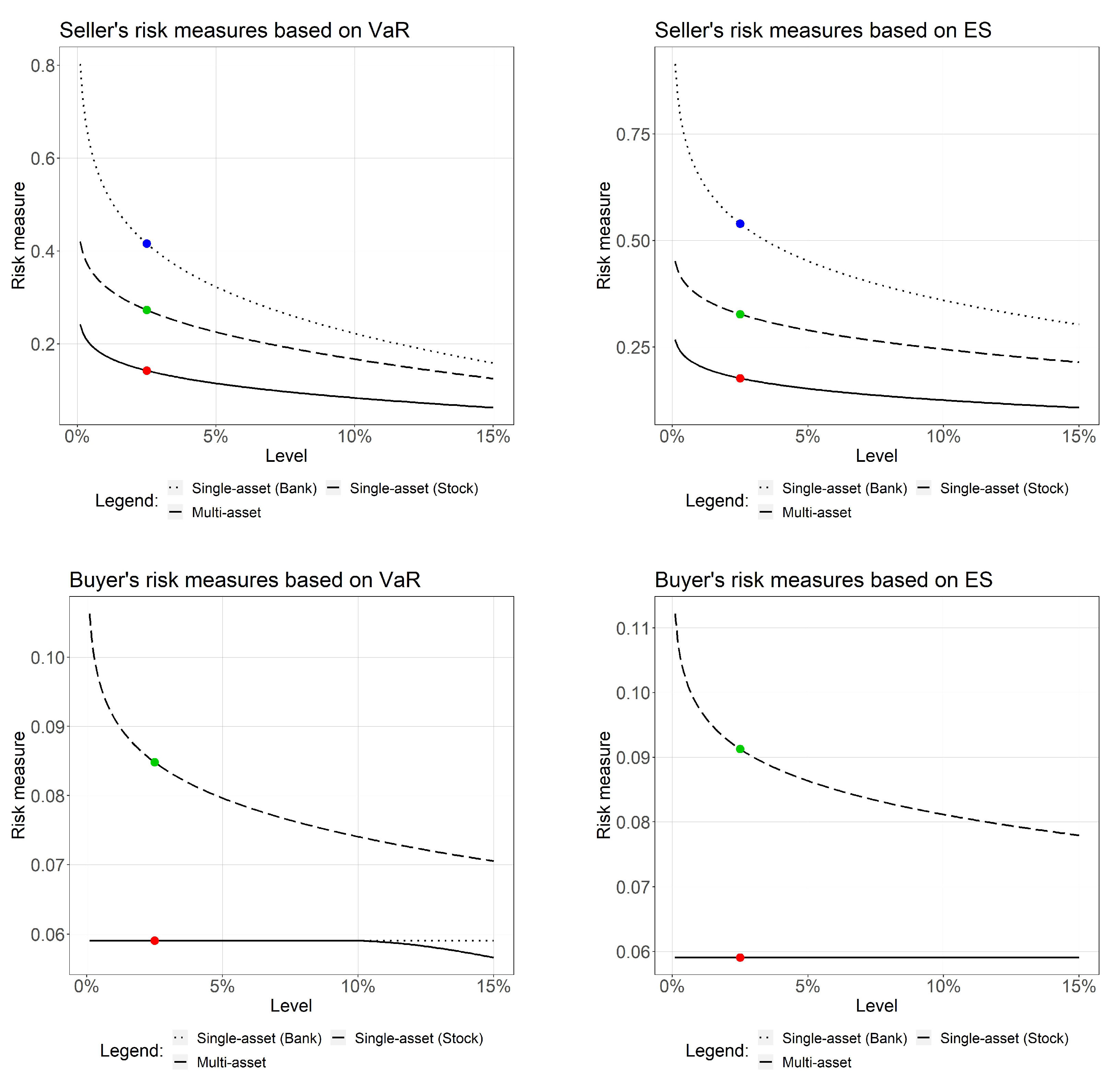
First, we compare the multi-asset risk measure with the single-asset risk measures based on the bank account and the stock. We plot them for different levels in Figure 1. The points correspond to the level $\lambda =2.5\%$. The plots for the VaR and the ES are quite similar. For the seller, there are significant differences between the three risk measures, that is, the multi-asset risk measure leads to a significantly smaller value. In contrast, the buyer’s multi-asset risk measure is in nearly every case equal to the single-asset risk measure w.r.t. the bank account. This is due to the fact that the long call position is already acceptable. If we would go short in the bank account, then the VaR and ES of the final payoff would be positive and therefore not acceptable. This means, the single-asset risk measure (dotted line) is equal to p.

For the multi-asset risk measure a short position in the stock is not meaningful, because the option is out-of-the money, that is, it is more likely that the option is not executed and the buyer relies on the loss of the short position. On the opposite, for lower strike values, short positions in the stock are hedged by the executed option with higher probability. This means, a short position in the stock would not necessarily lead to an unacceptable position and it is therefore also possible to reduce the capital requirement under the value of the single-asset risk measure w.r.t. the bank account.

The single-asset risk measure w.r.t. the stock (dashed line) is significantly larger than the other two risk measures. This is due to the fact that there is no kind of translation invariance property for the short position of the value p, that is, there is a high effort to secure the negative amount $-p$.

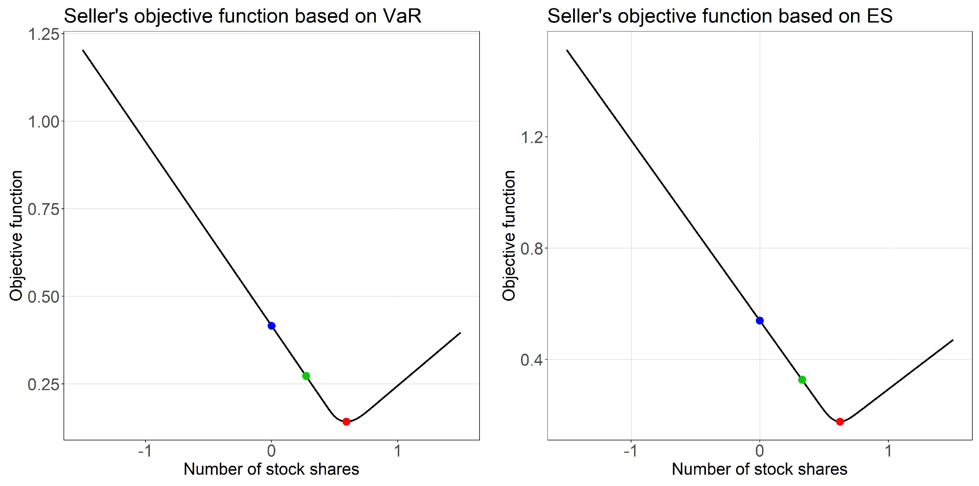
To get an intuition of the corresponding hedging strategies, we plot in Figure 2 the capital requirement in dependence on the number of stock shares, for example, for the seller we plot the following function:

$$\begin{array}{c}\hfill \mathbb{R}\to \mathbb{R},\phi \mapsto \phi S_0+\frac{{\rho }_{}\left(\phi S_T-X\right)}{B_T}{B}_0,\end{array}$$

with ${\rho }_{}\in \left\{{VaR}_{\lambda },{ES}_{\lambda }\right\}$ and level $\lambda =2.5\%$. The red point corresponds to the multi-asset risk measure. We see that there exists a unique optimal solution. The blue and the green points are the single-asset risk measures w.r.t. bank account and stock.

For the seller, hedging with the bank account is most expensive. Further, the multi-asset risk measure attains the minimum in the interior of the interval $\left[0,1\right]$. In contrast, the buyer does not need the additional hedging opportunity given by the stock, that is, the red point is overlapping the blue point.

4. Pricing with Multi-Asset Risk Measures

We use the previous results for multi-asset risk measures to obtain pricing bounds for European options. If a price is chosen within these bounds it is guaranteed that there are no trading strategies at zero costs s.t. the resulting portfolio would be acceptable.

In a first step, we define good-deals and illustrate pricing bounds based on VaR and ES acceptance sets. In a second step in Section 5, we show a duality relation. If this relation holds, there is an option price s.t. there are no good-deals on the extended market, that is, the market which allows for trading of the option.

4.1. Good-Deals of the First Kind

A good-deal is a payoff which is too profitable for a marketed agent. This means the market should not allow for such payoffs. As pointed out in Arai and Fukasawa (2014), there is a strong connection between risk measures and so-called good-deal bounds. We use the concept of no good-deals of the first kind as introduced in (Jaschke and Küchler 2001, Section 4).

Definition 5

(Good-deals of the first kind). Assume an acceptance set $\mathcal{A}\subset \mathcal{X}$. A payoff $X\in \mathcal{X}$ is a good-deal of the first kind, if $X\in \left(\mathcal{A}\cap {\mathcal{M}}_0\right)\backslash \left\{0\right\}$.

The following result admits an equivalent condition for the absence of good-deals of the first kind in the one-period BSM.

Lemma 4.

Let ${\rho }_{}$ be a positive homogeneous monetary risk measure. The absence of good-deals of the first kind w.r.t. the acceptance set ${\mathcal{A}}_{{\rho }_{}}$ is equivalent to the condition that

$$\begin{array}{c}\hfill \frac{B_T}{B_0}\in \left(\frac{-{\rho }_{}\left(S_T\right)}{S_0},\frac{{\rho }_{}\left(-S_T\right)}{S_0}\right).\end{array}$$

(16)

Proof. 

The absence of good-deals of the first kind is equivalent to the condition that for each $\phi \in \mathbb{R}\backslash \left\{0\right\}$ it holds that ${\rho }_{}\left(-\frac{\phi S_0}{B_0}{B}_T+\phi S_T\right)>0$. By this statement we are able to consider the cases of $\phi \in {\mathbb{R}}_{>0}$ and $\phi \in {\mathbb{R}}_{<0}$ s.t. we obtain the required equivalent statement of $\frac{B_T}{B_0}\in \left(\frac{-{\rho }_{}\left(S_T\right)}{S_0},\frac{{\rho }_{}\left(-S_T\right)}{S_0}\right)$. □

Remark 7.

(i) 

In a financial market model with multiple stocks $\widehat{S}$ the absence of good-deals of the first kind is equivalent to the condition that for each $\phi \in \partial B_{{\mathbb{R}}^d}$ it holds that $〈\frac{B_T}{B_0}{\widehat{S}}_0,\phi 〉<{\rho }_{}\left(-〈{\widehat{S}}_T,\phi 〉\right)$.

(ii) 

Lemma 4 shows that in our model the absence of good-deals of the first kind implies the absence of acceptability arbitrage, since (16) implies (10) which by Theorem 1 is equivalent to the absence of acceptability arbitrage opportunities. But this is not true in general, as the subsequent counterexample shows.

Example 4.

We present a setup in which the following implication does not hold in general:

$$\begin{array}{c}\hfill \left(\mathcal{A}\cap {\mathcal{M}}_0\right)\backslash \left\{0\right\}=\mathrm{⌀}\Rightarrow \mathcal{A}\cap {\mathcal{M}}_x=\mathrm{⌀}\mathrm{for}\mathrm{some}x\in \mathbb{R}.\end{array}$$

The only case in which this implication could fail is that $\mathcal{A}\cap {\mathcal{M}}_0=\left\{0\right\}$. We use a one-period BSM with marketed set $\mathcal{M}=span\left\{1_{\Omega }\right\}$, the pricing functional given by $\pi \left(\phi \right)=\phi$ and the acceptance set $\mathcal{A}={\bigcup }_{m\in \mathbb{R}}\left\{X\in L^1|X\ge mP-\mathrm{a}.\mathrm{s}.\right\}$. Then ${\mathcal{M}}_0=\left\{0\right\}$ implies that there are no good-deals of the first kind, because of $\mathcal{A}\cap {\mathcal{M}}_0=\mathcal{A}\cap \left\{0\right\}=\left\{0\right\}$. But the no acceptability arbitrage condition is not fulfilled, because for every $x\in \mathbb{R}$ we have

$$\begin{array}{c}\hfill \mathcal{A}\cap {\mathcal{M}}_x=\mathcal{A}\cap \left\{x{1}_{\Omega }\right\}=\left\{x{1}_{\Omega }\right\}\ne \mathrm{⌀},\end{array}$$

that is, the pricing functional π is unbounded on $\mathcal{A}\cap \mathcal{M}$.

4.2. Good-Deal Bounds for Option Prices

In the following we work under the assumption that the one-period BSM does not admit good-deals of the first kind. By Remark 7 (ii), then also the absence of acceptability arbitrage condition is satisfied. Let ${\rho }_{}\in \left\{{VaR}_{\lambda },{ES}_{\lambda }\right\}$ with level $\lambda \in \left(0,0.5\right)$. As described in Jaschke and Küchler (2001), the good-deal bounds for a call option are then given by ${\rho }_{{\mathcal{A}}_{{\rho }_{}},\mathcal{M},\pi }\left(-X\right)$ and $-{\rho }_{{\mathcal{A}}_{{\rho }_{}},\mathcal{M},\pi }\left(X\right)$. From our previous results we obtain:

$$\begin{array}{cccccccc}& \mathbf{Seller}:\hfill & & {\rho }_{{\mathcal{A}}_{{\rho }_{}},\mathcal{M},\pi }\left(-X\right)\hfill & & =\hfill & & \underset{\phi \in \left[0,1\right]}{inf}\left(\phi S_0+{\rho }_{}\left(\phi S_T-{\left(S_T-K\right)}^{+}\right)\frac{B_0}{B_T}\right),\hfill \end{array}$$

(17)

$$\begin{array}{cccccccc}& \mathbf{Buyer}:\hfill & & -{\rho }_{{\mathcal{A}}_{{\rho }_{}},\mathcal{M},\pi }\left(X\right)\hfill & & =\hfill & & -\underset{\phi \in \left[-1,0\right]}{inf}\left(\phi S_0+{\rho }_{}\left(\phi S_T+{\left(S_T-K\right)}^{+}\right)\frac{B_0}{B_T}\right).\hfill \end{array}$$

(18)

Remark 8.

Sub- and superhedging prices could be obtained by using the positive cone $L_{+}^1$ as acceptance set. It is possible to rewrite the buyer good-deal bound to emphasize the analogy to the subhedging price. For the VaR we get the following expression:

$$\begin{array}{c}\hfill -{\rho }_{{\mathcal{A}}_{{VaR}_{\lambda }},\mathcal{M},\pi }\left(X\right)=\underset{\phi \in \left[0,1\right]}{sup}\left(\phi S_0+{VaR}_{1-\lambda }\left(\phi S_T-{\left(S_T-K\right)}^{+}\right)\frac{B_0}{B_T}\right).\end{array}$$

(19)

In the following we calculate good-deal bounds for VaR and ES acceptance sets. For the sake of illustration, we choose a large level $\lambda$. This leads to plots demonstrating the advantage of the Expected Shortfall over the Value-at-Risk.

Example 5.

In Figure 3 we illustrate the good-deal bounds for the following parameters:

$$\begin{array}{c}\hfill T=1,B_0=1,r=0,\lambda =25\%,b=5\%,\sigma =20\%,K=1.\end{array}$$

The plots show the good-deal bounds as a function of the initial price of the underlying stock. Additionally, the prices using the Black-Scholes formula for instantaneous trading and the subhedging prices are given. Note that the no arbitrage price range is $\left(max\left\{0,S_0-K\right\},S_0\right)$. The plots are inspired by Cochrane and Saa-Requejo (2000) [Figure 1].

Compared with the Black-Scholes and subhedging price the good-deal bounds w.r.t. the ES do not admit an unexpected behavior. For the VaR the buyer good-deal bounds seem plausible. What is not directly intuitive is that the seller’s bound is sometimes lower than the buyer’s bound. For instance, this is the case for stock prices in the interval $\left[1.11,1.15\right]$. For a specific $\phi \in \left[0,1\right]$ and any $\lambda \in \left(0,0.5\right)$ we obtain:

$$\begin{array}{c}\hfill \phi S_0+{VaR}_{1-\lambda }\left(\phi S_1-{\left(S_1-K\right)}^{+}\right)\le \phi S_0+{VaR}_{\lambda }\left(\phi S_1-{\left(S_1-K\right)}^{+}\right).\end{array}$$

Nevertheless, we are not able to conclude that the seller’s bound is always greater or equal than the buyer’s bound as our counterexample shows. This undesirable behavior occurs if there does not exist an equivalent martingale measure s.t. the extended market is free of good-deals. We will discuss this fact in detail in Section 5.2 below.

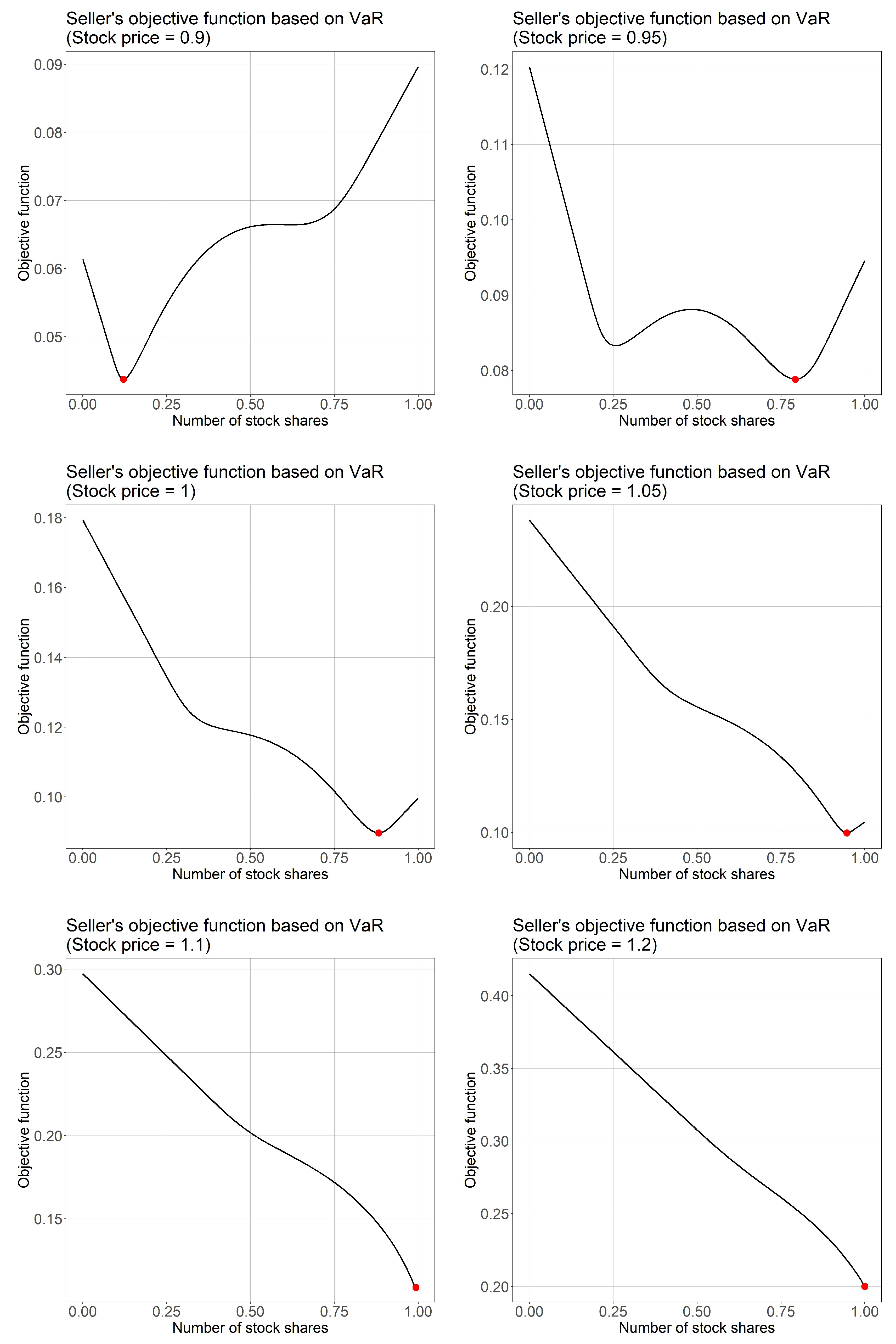
To provide more intuition on the shape of the seller’s good-deal bound based on VaR in Figure 3, in Figure 4 we plot the objective function from the optimization problem of the seller using VaR as preference criterion, that is, we plot the function $\phi \mapsto \phi S_0+{VaR}_{\lambda }\left(\phi S_1-{\left(S_1-K\right)}^{+}\right)$. Each plot corresponds to a specific stock price $S_0$. We see that the minimum for rising stock prices goes hand in hand with a rising number of stock shares. For the stock prices of $0.9$ and $0.95$ there are one local and one global minimum. For increasing stock prices in the interval $\left(0.9,0.95\right)$ the stock position belonging to the global minimum changes in a discontinuous manner, because at some stock price local and global minima change their roles. This is the reason for the kink of the seller good-deal bound in Figure 3.

Finally, we would like to elaborate on the level λ. Therefore, we alter the previous parameters in the following way:

$$\begin{array}{c}\hfill T=1,B_0=1,{\mathbf{S}}_{\mathbf{0}}=\mathbf{1}.\mathbf{12},r=0,b=5\%,\sigma =20\%,K=1.\end{array}$$

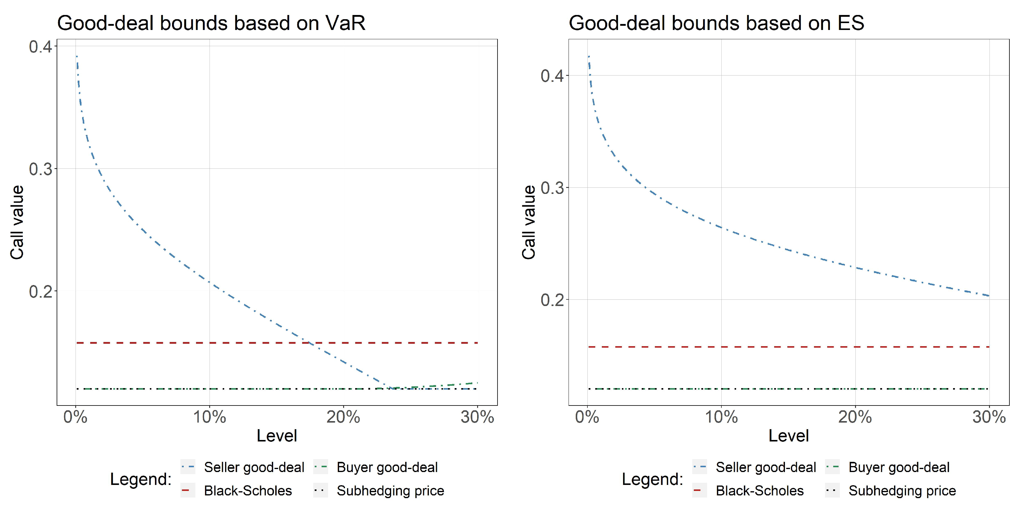
In Figure 5 we illustrate the good-deal bounds depending on the level λ. For the VaR acceptance set we see that only for high levels the seller’s price is lower than the buyer’s price.

4.3. Limiting Behavior

For increasing stock prices the seller’s good-deal bound in Figure 3 tends to the subhedging price. In this short subsection we give the reason for this behavior in the VaR-case. There is an intuitive explanation. If the stock price goes up the call option is deeper in-the-money. This results in the following two effects:

• It becomes more likely that the option is exercised, resulting in a loss for the seller.
• Higher losses for the seller become more probable.

Therefore, it is more expensive to hedge the short call position. As we have seen in Figure 4, the seller buys one stock share for high enough stock prices. Even if the seller goes short in the bank account, the future loss is bounded from below. The resulting seller good-deal bound is

$$\begin{array}{c}\hfill S_0+{VaR}_{\lambda }\left(S_1-{\left(S_1-K\right)}^{+}\right).\end{array}$$

(20)

If $\lambda >F_{S_1}\left(K\right)$, then

$$\begin{array}{c}\hfill S_0+{VaR}_{\lambda }\left(S_1-{\left(S_1-K\right)}^{+}\right)=S_0-K,\end{array}$$

(21)

that is, the seller’s bound is equal to the subhedging price. For large enough stock prices the condition is fulfilled, because of

$$\begin{array}{c}\hfill \underset{S_0\to \infty }{lim}{F}_{S_1}\left(K\right)=\underset{S_0\to \infty }{lim}\Phi \left(\frac{ln\left(K/S_0\right)-\left(b-{\sigma }^2/2\right)}{\sigma }\right)=0.\end{array}$$

(22)

An analog explanation holds for the case if the stock price tends to zero.

5. Extension of the Basis Market

In this section we explain why it can happen that the seller’s good-deal bound is smaller than the buyer’s good-deal bound using a VaR acceptance set. This is due to the failure of the so-called extension theorem for VaR. Subsequently, we prove the validity of the extension theorem for an ES acceptance set, showing that such a situation cannot happen for ES.

5.1. Duality Relations

We develop a duality relation for the seller’s good-deal bound w.r.t. an acceptance set based on a positive homogeneous monetary risk measure ${\rho }_{}$. Let ${\mathcal{P}}_{{\rho }_{}}\left(C\right)$ be the set of prices for a financial payoff $C\in \mathcal{X}$ s.t. there are no good-deals of the first kind in the extended market, that is, for $p\in {\mathcal{P}}_{{\rho }_{}}\left(C\right)$ there do not exist ${\phi }^S,{\phi }^C\in \mathbb{R}$ excluding the case ${\phi }^S={\phi }^C=0$ s.t.

$$\begin{array}{c}\hfill {\rho }_{}\left({\phi }^S\left(S_T-S_0\frac{B_T}{B_0}\right)+{\phi }^C\left(C-p\frac{B_T}{B_0}\right)\right)\le 0.\end{array}$$

(23)

By positive homogeneity of ${\rho }_{}$ we obtain that $L_{+}^1\subset \mathcal{A}$. This implies that every arbitrage opportunity is also a good-deal. Hence, the set ${\mathcal{P}}_{{\rho }_{}}\left(C\right)$ is a subset of the no arbitrage price range of C. Therefore, the set of no good-deal prices in the extended market can be characterized as a subset of all equivalent martingale measures. This subset of equivalent martingale measures is denoted by ${\mathcal{P}}_{{\rho }_{}}^{*}\left(C\right)$.

In the following we assume that there exists at least one price s.t. there are no good-deals in the extended market, that is, we work under the assumption

$$\begin{array}{c}\hfill {\mathcal{P}}_{{\rho }_{}}^{*}\left(C\right)\ne \mathrm{⌀}.\end{array}$$

(24)

Remark 9.

This condition implies that the basis market $\mathcal{M}$ satisfies the condition of the absence of good-deals of the first kind.

Now we are able to present the duality result. It is analog to the corresponding result for the superhedging price, see for example, (Föllmer and Schied 2016, Theorem 1.32).

Proposition 4.

The seller’s good-deal bound for a P-a.s. non-negative random variable C in the one-period BSM is given by

$$\begin{array}{c}\hfill {\rho }_{}\left(-C\right)=\underset{\phi \in \mathbb{R}}{inf}\left(\phi S_0+\frac{{\rho }_{}\left(\phi S_T-C\right)}{B_T}{B}_0\right)=\underset{P^{*}\in {\mathcal{P}}_{{\rho }_{}}^{*}\left(C\right)}{sup}{E}_{P^{*}}\left(C\right).\end{array}$$

(25)

Proof. 

From the discussion before we obtain that $\underset{P^{*}\in {\mathcal{P}}_{{\rho }_{}}^{*}\left(C\right)}{sup}{E}_{P^{*}}\left(C\right)=sup{\mathcal{P}}_{{\rho }_{}}\left(C\right)$. Assume there exists $\phi \in \mathbb{R}$ s.t. for a value $m\in \mathbb{R}$ it holds that ${\rho }_{}\left(m\frac{B_T}{B_0}+\phi \left(S_T-S_0\frac{B_T}{B_0}\right)-C\right)\le 0$. From cash invariance we obtain $\frac{B_0}{B_T}{\rho }_{}\left(\phi \left(S_T-S_0\frac{B_T}{B_0}\right)-C\right)\le m$. Therefore, every $p\ge m$ cannot be a price in the extended market s.t. there does not exist a good-deal. This implies ${\rho }_{}\left(-C\right)\ge sup{\mathcal{P}}_{{\rho }_{}}\left(C\right)$.

It is left to show that for every $m>sup{\mathcal{P}}_{{\rho }_{}}\left(C\right)$ it holds that $m\ge {\rho }_{}\left(-C\right)$. Therefore, assume $m>sup{\mathcal{P}}_{{\rho }_{}}\left(C\right)$. There are ${\phi }^S,{\phi }^C\in \mathbb{R}$ excluding the case ${\phi }^S={\phi }^C=0$ such that

$$\begin{array}{c}\hfill {\rho }_{}\left({\phi }^S\left(S_T-S_0\frac{B_T}{B_0}\right)+{\phi }^C\left(C-m\frac{B_T}{B_0}\right)\right)\le 0.\end{array}$$

The basis market does not admit good-deals of the first kind. This implies ${\phi }^C\ne 0$. If ${\phi }^C<0$, we obtain from the positive homogeneity of ${\rho }_{}$ that

$$\begin{array}{c}\hfill {\rho }_{}\left(m\frac{B_T}{B_0}-\frac{{\phi }^S}{{\phi }^C}\left(S_T-S_0\frac{B_T}{B_0}\right)-C\right)\le 0.\end{array}$$

It remains to show that the case ${\phi }^C>0$ is not feasible. We know that there exists a price $p\in {\mathcal{P}}_{{\rho }_{}}\left(C\right)$ for each $a,b\in \mathbb{R}$ excluding the case $a=b=0$ and we have

$$\begin{array}{c}\hfill {\rho }_{}\left(a\left(S_T-S_0\frac{B_T}{B_0}\right)+b\left(C-p\frac{B_T}{B_0}\right)\right)>0.\end{array}$$

At the same time positive homogeneity of ${\rho }_{}$ implies

$$\begin{array}{c}\hfill {\rho }_{}\left(\frac{{\phi }^S}{{\phi }^C}\left(S_T-S_0\frac{B_T}{B_0}\right)+C-m\frac{B_T}{B_0}\right)\le 0.\end{array}$$

These two statements together with monotonicity of ${\rho }_{}$ and $m>p$ imply

$$\begin{array}{c}\hfill 0\ge {\rho }_{}\left(\frac{{\phi }^S}{{\phi }^C}\left(S_T-S_0\frac{B_T}{B_0}\right)+C-m\frac{B_T}{B_0}\right)>{\rho }_{}\left(\frac{{\phi }^S}{{\phi }^C}\left(S_T-S_0\frac{B_T}{B_0}\right)+C-p\frac{B_T}{B_0}\right)>0,\end{array}$$

which is a contradiction. □

Remark 10.

A corresponding result holds for the buyer’s good-deal bound:

$$\begin{array}{c}\hfill {\rho }_{}\left(-C\right)=\underset{P^{*}\in {\mathcal{P}}_{{\rho }_{}}^{*}\left(C\right)}{sup}{E}_{P^{*}}\left(C\right)\ge \underset{P^{*}\in {\mathcal{P}}_{{\rho }_{}}^{*}\left(C\right)}{inf}{E}_{P^{*}}\left(C\right)=-{\rho }_{}\left(C\right).\end{array}$$

(26)

5.2. Failure of the Extension Theorem

If we go back to Figure 3, we are now able to answer the question why the seller’s bound w.r.t. the VaR is lower than the buyer’s bound. If we recall Remark 10, then we know that this is only possible if

$$\begin{array}{c}\hfill {\mathcal{P}}_{{VaR}_{\lambda }}^{*}\left({\left(S_T-K\right)}^{+}\right)=\mathrm{⌀}.\end{array}$$

(27)

This means that there is no price s.t. the extended market is free of good-deals of the first kind. This must also hold if there are no good-deals of the first kind on the basis market $\mathcal{M}$. From lemma 4, we obtain that the absence of good-deals on the basis market is equivalent to

$$\begin{array}{c}\hfill \frac{B_T}{B_0}\in \left(\frac{q_{S_T}^{+}\left(\lambda \right)}{S_0},\frac{q_{S_T}^{+}\left(1-\lambda \right)}{S_0}\right).\end{array}$$

(28)

This condition is independent of the stock price and is in particular fulfilled in Example 5. The situation that every possible option price leads to an extended market which is not free of good-deals means that for every price $p\in \mathbb{R}$ there exists $\theta \in \mathbb{R}$ such that

$$\begin{array}{c}\hfill \theta S_0+{VaR}_{\lambda }\left(\theta S_T+{\left(S_T-K\right)}^{+}\right)\frac{B_T}{B_0}\le -p,\end{array}$$

(29)

or

$$\begin{array}{c}\hfill \theta S_0+{VaR}_{1-\lambda }\left(\theta S_T+{\left(S_T-K\right)}^{+}\right)\frac{B_T}{B_0}\ge -p.\end{array}$$

(30)

In contrast to the basis market the absence of good-deals of the first kind depends on the stock price. For $\theta =1$, the earlier argument that the seller’s good-deal bound converges to the subhedging price, could be used in an analog way to show that for high enough stock prices both VaR expressions in the previous inequalities are equal to the subhedging price $S_0-K$. Hence, one of the above conditions is fulfilled for large enough stock prices.

Remark 11.

The extension theorem as described in (Černý and Hodges 2002, Section 2.1) states, that a basis market which is free of good-deals could be extended s.t. the extended market, is free of good-deals of the first kind. But this would be a contradiction to our Value-at-Risk example, that is, a contradiction to ${\mathcal{P}}_{{VaR}_{\lambda }}^{*}\left({\left(S_T-K\right)}^{+}\right)=\mathrm{⌀}$. Therefore, a sufficient assumption in the extension theorem is not satisfied. In fact, in our setting the VaR acceptance set is not boundedly generated2^,3. This is intuitive, because the proof of the extension theorem is based on a separation argument. Such a separation is likely to fail if the acceptance set is not convex, like in the VaR-case.

The previous remark raises the question if the extension theorem holds for the ES acceptance set. This is indeed the case. The reason is that the convexity of the acceptance set allows for a separation argument to extend the pricing functional to the whole space of contingent claims. The arguments in the following proof are in line with the ones in the Proof of Theorem 2.3 in Černý and Hodges (2002). Nevertheless, our setup differs slightly from the one in Černý and Hodges (2002), for example, the intersection of ${\mathcal{M}}_0$ and $\mathcal{A}$ could contain the zero vector, which is not the case in Černý and Hodges (2002). Furthermore, our proof does not explicitly use the condition of a boundedly generated set and we apply the Interior Separating Hyperplane Theorem instead of relying on the Hahn-Banach Theorem.

Theorem 4

(Expected Shortfall extension theorem). Assume the one-period BSM model and good-deals defined by the ES acceptance set w.r.t. a level $\lambda \in \left(0,0.5\right)$. Assume that there are no good-deals of the first kind on the basis market $\mathcal{M}$. In this setup, there exists an extension of the pricing functional $\pi :\mathcal{M}\to \mathbb{R}$ to the whole space of financial payoffs $\mathcal{X}$ s.t. there are no good-deals in the extended market.

Proof. 

From (Farkas et al. 2014, Lemma 4.3) we obtain

$$\begin{array}{c}\hfill {int}_{}\left({\mathcal{A}}_{{ES}_{\lambda }}\right)=\left\{X\in \mathcal{X}|{ES}_{\lambda }\left(X\right)<0\right\}.\end{array}$$

This shows that $0\notin {int}_{}\left({\mathcal{A}}_{{ES}_{\lambda }}\right)$, which in turn implies that ${int}_{}\left({\mathcal{A}}_{{ES}_{\lambda }}\backslash \left\{0\right\}\right)={int}_{}\left({\mathcal{A}}_{{ES}_{\lambda }}\right)$. Again, from (Farkas et al. 2014, Lemma 4.3) we obtain $S_T\in {int}_{}\left({\mathcal{A}}_{{ES}_{\lambda }}\right)$. A straightforward calculation gives that ${\mathcal{A}}_{{ES}_{\lambda }}\backslash \left\{0\right\}$ is convex. The assumption of no good-deals of the first kind on the basis market states that $\left({\mathcal{A}}_{{ES}_{\lambda }}\cap {\mathcal{M}}_0\right)\backslash \left\{0\right\}=\mathrm{⌀}$. Summarizing, ${\mathcal{A}}_{{ES}_{\lambda }}\backslash \left\{0\right\}$ and ${\mathcal{M}}_0$ are two non-empty, disjoint, convex sets for which ${\mathcal{A}}_{{ES}_{\lambda }}\backslash \left\{0\right\}$ contains an interior point. Therefore, by the Interior Separating Hyperplane Theorem (see e.g. (Aliprantis and Border 2006, Theorem 5.67)) there exists a non-zero continuous functional p which properly separates these two sets.

Since ${\mathcal{M}}_0$ is a subspace, we obtain for each $x\in {\mathcal{M}}_0$ that $p\left(x\right)=0$ and additionally we could assume that for each $x\in {\mathcal{A}}_{{ES}_{\lambda }}\backslash \left\{0\right\}$ it holds that $p\left(x\right)\ge 0$. Since the separation is proper, there exists $y\in {\mathcal{A}}_{{ES}_{\lambda }}\backslash \left\{0\right\}$ with $p\left(y\right)>0$.

Note, that every $x\in {\mathcal{A}}_{{ES}_{\lambda }}\backslash \left\{0\right\}$ obtains a representation with $\alpha \in \mathbb{R},s\in \left[p=0\right]$ s.t. $x=\alpha y+s$. This implies $p\left(x\right)=\alpha p\left(y\right)$. The scalar $\alpha$ cannot be zero ($x\notin {\mathcal{M}}_0$) and also not negative ($p\left(x\right)\ge 0$). Hence, it holds that $p\left(x\right)>0$ and the usage of p as pricing functional in the extended market would exclude good-deals. It also would exclude arbitrage opportunities, because of $L_{+}^1\subset {\mathcal{A}}_{{ES}_{\lambda }}$. But, we are not allowed to use p directly as extended pricing functional. This is due to the fact that p could price the basis assets in a different way than before, that is, $p\left({\phi }^B{B}_T+{\phi }^S{S}_T\right)\ne {\phi }^B{B}_0+{\phi }^S{S}_0$. We obtain a suitable functional $\tilde{p}$ by rescaling p with $p\left(B_T\right)/B_0$, that is, for each $x\in L^1$ we set $\tilde{p}\left(x\right)=\frac{p\left(x\right)}{p\left(B_T\right)}{B}_0$. □

6. Conclusions and Outlook

We study good-deal bounds based on Value-at-Risk and Expected Shortfall acceptance sets. Based on a benchmark example we demonstrate that the Value-at-Risk good-deal bounds for a European type call option behave non-smooth under varying the underlying stock price. We find that the reason for this is a jump in the optimal hedging strategy. The application of the Expected Shortfall does not admit this discontinuous behavior. Additionally, in the Value-at-Risk case, the seller’s bound is sometimes smaller than the buyer’s bound. To explain this, we show that the extension theorem in Černý and Hodges (2002) is not applicable in the non-convex Value-at-Risk case. In addition, we present new finiteness and continuity results for risk measures based on multiple eligible assets in our concrete setup.

These results depend on the one-period Black-Scholes market model. Therefore, a future direction of research could be to incorporate a market with more than one risky asset, for which we gave a short outlook in the Remarks 5 and 7. Also the use of intermediate trading strategies is a natural extension of our setup.

References

1. Aliprantis, Charalambos D., and Kim C. Border. 2006. Infinite Dimensional Analysis: A Hitchhiker’s Guide, 3rd ed. Berlin and Heidelberg: Springer. [Google Scholar] [CrossRef]
2. Arai, Takuji. 2011. Good Deal Bounds Induced by Shortfall Risk. SIAM Journal on Financial Mathematics 2: 1–21. [Google Scholar] [CrossRef] [Green Version]
3. Arai, Takuji, and Masaaki Fukasawa. 2014. Convex Risk Measures for Good Deal Bounds. Mathematical Finance 24: 464–84. [Google Scholar] [CrossRef] [Green Version]
4. Artzner, Philippe, Freddy Delbaen, Jean-Marc Eber, and David Heath. 1999. Coherent Measures of Risk. Mathematical Finance 9: 203–28. [Google Scholar] [CrossRef]
5. Artzner, Philippe, Freddy Delbaen, and Pablo Koch-Medina. 2009. Risk Measures and Efficient use of Capital 1. ASTIN Bulletin: The Journal of the IAA 39: 101–16. [Google Scholar] [CrossRef] [Green Version]
6. Baes, Michel, Pablo Koch-Medina, and Cosimo Munari. 2020. Existence, uniqueness, and stability of optimal payoffs of eligible assets. Mathematical Finance 30: 128–66. [Google Scholar] [CrossRef] [Green Version]
7. Bernardo, Antonio E., and Olivier Ledoit. 2000. Gain, Loss, and Asset Pricing. Journal of Political Economy 108: 144–72. [Google Scholar] [CrossRef] [Green Version]
8. Björk, Tomas, and Irina Slinko. 2006. Towards a General Theory of Good-Deal Bounds. Review of Finance 10: 221–60. [Google Scholar] [CrossRef]
9. Carr, Peter, Helyette Geman, and Dilip B. Madan. 2001. Pricing and hedging in incomplete markets. Journal of Financial Economics 62: 131–67. [Google Scholar] [CrossRef]
10. Cheridito, Patrick, and Tianhui Li. 2009. Risk Measures on Orlicz Hearts. Mathematical Finance 19: 189–214. [Google Scholar] [CrossRef]
11. Cochrane, John H., and Jesus Saa-Requejo. 2000. Beyond Arbitrage: Good-Deal Asset Price Bounds in Incomplete Markets. Journal of Political Economy 108: 79–19. [Google Scholar] [CrossRef] [Green Version]
12. Cox, John C., Stephen A. Ross, and Mark Rubinstein. 1979. Option pricing: A simplified approach. Journal of Financial Economics 7: 229–63. [Google Scholar] [CrossRef]
13. Farkas, Walter, Pablo Koch-Medina, and Cosimo Munari. 2014. Beyond cash-additive risk measures: When changing the numéraire fails. Finance and Stochastics 18: 145–73. [Google Scholar] [CrossRef] [Green Version]
14. Farkas, Walter, Pablo Koch-Medina, and Cosimo Munari. 2015. Measuring risk with multiple eligible assets. Mathematics and Financial Economics 9: 3–27. [Google Scholar] [CrossRef] [Green Version]
15. Föllmer, Hans, and Alexander Schied. 2016. Stochastic Finance: An Introduction in Discrete Time. Berlin and Boston: Walter de Gruyter. [Google Scholar]
16. Geissel, Sebastian, Jörn Sass, and Frank Thomas Seifried. 2018. Optimal expected utility risk measures. Statistics & Risk Modeling 35: 73–87. [Google Scholar] [CrossRef]
17. Jaschke, Stefan, and Uwe Küchler. 2001. Coherent risk measures and good-deal bounds. Finance and Stochastics 5: 181–200. [Google Scholar] [CrossRef]
18. Larsen, Kasper, Traian A. Pirvu, Steven E. Shreve, and Reha Tütüncü. 2005. Satisfying convex risk limits by trading. Finance and Stochastics 9: 177–95. [Google Scholar] [CrossRef]
19. Liebrich, Felix-Benedikt, and Gregor Svindland. 2017. Model spaces for risk measures. Insurance: Mathematics and Economics 77: 150–65. [Google Scholar] [CrossRef] [Green Version]
20. Liebrich, Felix-Benedikt, and Gregor Svindland. 2019. Risk sharing for capital requirements with multidimensional security markets. Finance and Stochastics 23: 925–73. [Google Scholar] [CrossRef] [Green Version]
21. Munari, Cosimo-Andrea. 2015. Measuring Risk Beyond the Cash-Additive Paradigm. Ph.D. Thesis, ETH Zurich, Zurich, Switzerland. [Google Scholar]
22. R Core Team. 2020. R: A Language and Environment for Statistical Computing. Vienna: R Foundation for Statistical Computing. [Google Scholar]
23. Scandolo, Giacomo. 2004. Models of Capital Requirements in Static and Dynamic Settings. Economic Notes 33: 415–35. [Google Scholar] [CrossRef]
24. Staum, Jeremy. 2004. Fundamental Theorems of Asset Pricing for Good Deal Bounds. Mathematical Finance 14: 141–61. [Google Scholar] [CrossRef]
25. Wang, Ruodu, and Ričardas Zitikis. 2020. An Axiomatic Foundation for the Expected Shortfall. Management Science. Published online in Articles in Advance 14 Sepertember 2020. [Google Scholar] [CrossRef]
26. Černý, Aleš. 2003. Generalised Sharpe Ratios and Asset Pricing in Incomplete Markets. Review of Finance 7: 191–233. [Google Scholar] [CrossRef]
27. Černý, Aleš, and Stewart Hodges. 2002. The Theory of Good-Deal Pricing in Financial Markets. In Mathematical Finance—Bachelier Congress 2000: Selected Papers from the First World Congress of the Bachelier Finance Society, Paris, June 29–July 1, 2000. Edited by Hélyette Geman, Dilip Madan, Stanley R. Pliska and Ton Vorst. Finance, Berlin and Heidelberg: Springer, pp. 175–202. [Google Scholar] [CrossRef]
1.
For comonotonic risk measures we refer to (Föllmer and Schied 2016, Section 4.7).
2.
Let K be a convex set of claims disjoint from the origin. It is called boundedly generated if there exists a closed bounded subset B K s.t. any point in K can be regarded as a scalar multiple of a point in B, see (Černý and Hodges 2002, Definition 2.2).
3.
Nevertheless, the VaR acceptance set is closed in L p , see (Munari 2015, Proposition 2.4.5).
Figure 1. Single-asset and multi-asset risk measures depending on the level λ.
Risks 08 00114 g001
Figure 2. Capital requirements depending on the number of stock shares.
Risks 08 00114 g002aRisks 08 00114 g002b
Figure 3. Good-deal bounds depending on the stock price
Risks 08 00114 g003
Figure 4. Seller’s objective function for different stock prices.
Risks 08 00114 g004
Figure 5. Good-deal bounds depending on the level λ.
Risks 08 00114 g005
Publisher’s Note: MDPI stays neutral with regard to jurisdictional claims in published maps and institutional affiliations.