Multivariate General Compound Point Processes in Limit Order Books

Abstract

In this paper, we focus on a new generalization of multivariate general compound Hawkes process (MGCHP), which we referred to as the multivariate general compound point process (MGCPP). Namely, we applied a multivariate point process to model the order flow instead of the Hawkes process. The law of large numbers (LLN) and two functional central limit theorems (FCLTs) for the MGCPP were proved in this work. Applications of the MGCPP in the limit order market were also considered. We provided numerical simulations and comparisons for the MGCPP and MGCHP by applying Google, Apple, Microsoft, Amazon, and Intel trading data.

1. Introduction

In this paper, we introduced a new class of stochastic models, which can be considered as a generalization of the multivariate general compound Hawkes process (MGCHP) in Guo and Swishchuk (2020). We called this model the multivariate general compound point processes (MGCPP). A Law of Large Numbers (LLN) and two Functional Central Limit Theorems (FCLT) for MGCPP were proved. FCLTs of the MGCPP can be viewed as a link between price volatility and the order flow. Thus, we applied this asymptotic method to study the mid-price modeling in the limit order book (LOB).

Hawkes process was applied to financial modelling for the first time in 2007 Bowsher (2007). Bacry et al. (2013) proved a LLN and FCLT for multivariate Hawkes process and applied them to study some economic phenomenons in 2013. Volatilities between five stocks were estimated by a 5-dimensional Hawkes process in Bauwens and Hautsch (2009) in 2009. Other types of Hawkes processes have been studied widely as well. The nonlinear Hawkes process was considered by Brémaud and Massoulié (1996) and the corresponding FCLT was proved in Zhu (2013). Some applications of multivariate Hawkes process to financial data are given in Embrechts et al. (2011). The regime-switching Hawkes process was considered by Vinkovskaya (2014) to describe the dynamics dependency on the bid–ask spread in limit order book. In Swishchuk and Vadori (2017), a semi-Markov process based on a renewal process was applied to the mid-price modeling in LOB. Swishchuk et al. (2017) also considered the general case of the semi-Markovian models in 2017. A good textbook for algorithmic and High-Frequency trading methods was written by Cartea et al. (2015) in 2015. Zheng et al. (2014) introduced a multivariate point process describing the dynamics of the Bid and Ask price of a financial asset. The point process is similar to a Hawkes process, with additional constraints on its intensity corresponding to the natural ordering of the best Bid and Ask prices. Chen et al. (2019) developed a new approach for investigating the properties of the Hawkes process without the restriction to mutual excitation or linear link functions. They employed a thinning process representation and a coupling construction to bound the dependence coefficient of the Hawkes process. Using recent developments on weakly dependent sequences, a concentration inequality for second-order statistics of the Hawkes process was established. This concentration inequality was applied to cross-covariance analysis in the high-dimensional regime, and it was verified the theoretical claims with simulation studies. A framework for fitting multivariate Hawkes process for large-scale problems (long history and a wide variety of events) was proposed by Lemonnier et al. (2017). Liniger thesis addresses theoretical and practical questions arising in connection with multivariate, marked, linear Hawkes process Liniger (2009). Yang et al. (2017) developed a nonparametric and online learning algorithm that estimates the triggering functions of a multivariate Hawkes process. An introduction to point processes from a martingale point of view may be found in Bjork’s lecture notes Bjork (2011).

Guo and Swishchuk (2020) constructed a multivariate general compound Hawkes process (MGCHP) which is an extended model from Cont and De Larrard (2013) and Swishchuk (2017). In Guo and Swishchuk (2020), they applied the multivariate Hawkes process to model the order flow of several stocks in limit order market and proved limit theorems for the MGCHP. In this paper, we proposed a new mid-price model which is a generalization of the MGCHP and we called it the multivariate general compound point process (MGCPP). For the MGCPP, we applied a multi-dimensional simple point process to represent the order flow in LOB instead of the Hawkes process. We also proved the corresponding LLN and FCLTs for the MGCPP. One of the reasons why we considered the generalized model is parameters for simple point process are much easier to estimate than Hawkes process. So, we provided the numerical comparisons of the MGCPP and MGCHP by real high-frequency trading data and we found that results of the new generalized model are as good as the MGCHP.

This paper is organized as follows. Definitions and assumptions of the multivariate general compound point process (MGCPP) can be found in Section 2. Functional central limit theorem (FCLT) I and law of large numbers were proved in Section 3. We also provided numerical examples simulated by real data for the FCLT I in Section 3. In Section 4, we considered a FCLT II for the MGCPP and applied it in the mid-price prediction. Section 5 concludes the paper.

2. Definition of Multivariate General Compound Point Process (MGCPP)

In this Section, we proposed a multivariate stochastic model for the mid-price in the limit order book. This is a generalization for models in Cont and De Larrard (2013), Guo and Swishchuk (2020), and Swishchuk (2017). Here, we assume the order flow was described by a multivariate simple point process with some good asymptotic properties.

Definition 1

((Counting Process). (see, e.g., Bjork (2011))). We called a stochastic process $\left\{N\right(t),t\ge 0\}$ counting process if it satisfies: the trajectories of $N_t$ are right continues and piecewise constant with probability one, $N\left(0\right)=0$, and $\Delta N_t=N_t-N_{t-}=0$ or 1 with probability one.

Counting process is the simplest type of point process. In the following discussion of paper, we adopt Definition 1 as the definition of a point process. The point process can be determined by the conditional intensity function λ(t) in the form of

$$\lambda \left(t\right)=\underset{h\to 0}{lim}\frac{E[N(t+h)-N\left(t\right)|{\mathcal{F}}^N\left(t\right)]}{h},$$

(1)

where λ(t) ≥ 0 and ${\mathcal{F}}^N\left(t\right)$ is the corresponding natural filtration.

2.1. Assumptions for Multivariate Point Processes

Let ${\overrightarrow{N}}_t=(N_{1,t},N_{2,t},\cdots ,N_{d,t},)$ be d-dimensional point process with following assumptions:

Assumption 1.

We assume there’s a law of large numbers (LLN) of the ${\overrightarrow{N}}_t$ in the form of:

$$\frac{\overrightarrow{N}\left(nt\right)}{n}\to \overrightarrow{\overline{\lambda }}t$$

(2)

as $n\to +\infty$ almost surely, where $\overrightarrow{\overline{\lambda }}=({\overline{\lambda }}_1,{\overline{\lambda }}_2,{\overline{\lambda }}_3,\cdots ,{\overline{\lambda }}_d)$.

Assumption 2.

We also assume there’s a Functional Central Limit Theorem (FCLT) of the ${\overrightarrow{N}}_t$ in the form of:

$$\frac{1}{\sqrt{n}}({\overrightarrow{N}}_{nt}-E\left({\overrightarrow{N}}_{nt}\right))\stackrel{n\to \infty }{\to }{\Sigma }^{1/2}{\overrightarrow{W}}_t,t\in [0,1]$$

(3)

in law of the Skorohod topology, where ${\overrightarrow{W}}_t$ is a standard d-dimensional Brownian motion and Σ is a d-by-d covariance matrix.

Here, $\overrightarrow{N_t}$ denotes the order flow in the limit order market for d stocks. Liquidity for the high-frequency trading data guarantees there are enough price changes in one day or even a small window size $nt$. So, it is reasonable to consider those two limit assumptions in the limit order book modeling.

Remark 1.

For a simple example, if we consider the point process as a multivariate homogeneous Poisson process with independent coordinates, then two assumptions above are LLN and FCLT for the multi-dimensional Poisson process. Let ${\overrightarrow{P}}_t$ be a d-dimensional Poisson process with intensity $\overrightarrow{\lambda }$. Here, we used notation ${\overrightarrow{P}}_t$ to distinguish the general case and the Poisson example. Then, we have the LLN in the form of

$$su{p}_{t\in [0,1]}∥n^{-1}{\overrightarrow{P}}_{nt}-t\overrightarrow{\lambda }∥\to 0$$

(4)

as $n\to \infty$ almost surely. Further, the FCLT in the form of

$$\sqrt{n}\left(\frac{1}{n}{\overrightarrow{P}}_{nt}-t\overrightarrow{\lambda }\right)$$

converge in law for the Skorokhod topology to ${\overrightarrow{W}}_t\circ {\overrightarrow{\lambda }}^{1/2}$ as $n\to \infty$, where ∘ is the element-wise product.

Remark 2.

Another interesting example is limit theorems for the multivariate Hawkes process (MHP) in Bacry et al. (2013). Let ${\overrightarrow{H}}_t=(H_{1,t},H_{2,t},\cdots ,H_{d,t})$ be a d-dimensional Hawkes process. The intensity function for each H_i is in the form of

$${\lambda }_i\left(t\right)={\lambda }_i+{\int }_{(0,t)}\sum _{j=1}^d{\mu }_{ij}(t-s)d{H}_{j,s},$$

(5)

Let $\mu ={\left({\mu }_{ij}\right)}_{1\le i,j\le d}$, $\overrightarrow{\lambda }={({\lambda }_1,{\lambda }_2,\cdots ,{\lambda }_d)}^T$, and $\mathbf{K}={\int }_0^{\infty }\mu \left(t\right)dt$, then the LLN for MHP is in the form of

$$su{p}_{t\in [0,1]}∥n^{-1}{\overrightarrow{H}}_{nt}-t{(\mathbf{I}-\mathbf{K})}^{-1}\overrightarrow{\lambda }∥\to 0$$

(6)

as $n\to \infty$ almost surely, where $\mathbf{I}$ is a d-by-d identity matrix. We can also have the FCLT for MHP:

$$\frac{1}{\sqrt{n}}({\overrightarrow{H}}_{nt}-E\left({\overrightarrow{H}}_{nt}\right))\stackrel{n\to \infty }{\to }{(\mathbf{I}-\mathbf{K})}^{-1}{\mathbf{D}}^{1/2}{\overrightarrow{W}}_t,t\in [0,1]$$

in law of the Skorohod topology, where ${\overrightarrow{W}}_t$ is a standard d-dimensional Brownian motion and $\mathbf{D}$ is a diagonal matrix determined by ${\mathbf{D}}_{ii}={\left({(\mathbf{I}-\mathbf{K})}^{-1}\overrightarrow{\lambda }\right)}_i$. Details about the LLN and FCLT of MHP can be found in Bacry et al. (2013).

2.2. Definition for MGCPP

Next, we consider a price process $\overrightarrow{S_t}$ in the form ${\overrightarrow{S}}_t=(S_{1,t},S_{2,t},\cdots ,S_{d,t},)$ as:

$$S_{i,t}=S_{i,0}+\sum _{k=1}^{N_{i,t}}{a}_i\left(X_{i,k}\right),$$

(7)

where $X_{i,k}$ are independent ergodic continuous-time Markov chains, independent of ${\overrightarrow{N}}_t$. The state space of $X_{i,k}$ is denoted by $X^{\left\{i\right\}}=\{1,2,\cdots ,{\mathcal{N}}_i\}$. $a_i(·)$ are bounded continuous functions. We refer $\overrightarrow{S_t}$ as multivariate general compound point processes (MGCPP).

Remark 3.

If we consider the one-dimensional case, let $N_t$ be a Poisson process, $a_i\left(x\right)=(-\delta )\vee (x\wedge \delta )$, and $X_k$ is a sequence of independent random variables such that $P(X_1=\delta )=P(X_1=-\delta )=1/2$, then $S_t$ is a stochastic model for the dynamics of a limit order book discussed in Cont and De Larrard (2013).

Remark 4.

When ${\overrightarrow{N}}_t$ is a multivariate Hawkes process in Remark 2, then ${\overrightarrow{S}}_t$ is a multivariate general compound Hawkes processes (MGCHP) which proposed in Guo and Swishchuk (2020).

3. LLNs and Diffusion Limits for MGCPP

In this Section, we considered the diffusion limit theorems for the MGCPP. It provides us a link between the order flow ${\overrightarrow{N}}_t$ and the price process ${\overrightarrow{S}}_t$. The functional central limit theorem (FCLT) and law of large numbers (LLN) for the MGCPP are generalizations for the diffusion limit theorems of the MGCHP in Guo and Swishchuk (2020).

3.1. LLN for MGCPP

Theorem 1

(LLN for MGCPP). Let ${\overrightarrow{S}}_{nt}=(S_{1,nt},S_{2,nt},S_{3,nt},\cdots ,S_{d,nt})$ be a d-dimensional MGCPP defined before, we have

$$\frac{{\overrightarrow{S}}_{nt}}{n}\to \widetilde{a^{*}}\overrightarrow{\overline{\lambda }}t$$

as $n\to \infty$ almost surely.

Proof of Theorem 1.

From the definition of MGCPP in Equation (7), we have

$$\frac{S_{i,nt}}{n}=\frac{S_{i,0}}{n}+\sum _{k=1}^{N_{i,nt}}\frac{a_i\left(X_{i,k}\right)}{n}.$$

Since $S_{i,0}$ is a constant, we have

$$\begin{array}{cc}\hfill \underset{n\to \infty }{lim}\left(\frac{S_{i,t}}{n}\right)& =\underset{n\to \infty }{lim}\left(\frac{S_{i,0}}{n}\right)+\underset{n\to \infty }{lim}\frac{{\sum }_{k=1}^{N_{i,nt}}{a}_i\left(X_{i,k}\right)}{n}\hfill \\ & =0+\underset{n\to \infty }{lim}\frac{{\sum }_{k=1}^{N_{i,nt}}{a}_i\left(X_{i,k}\right)}{n}.\hfill \end{array}$$

(8)

Recall the strong LLN of Markov chain (see, e.g., Norris (1998)), we have

$$\frac{1}{n}\sum _{k=1}^n{a}_i\left(X_{i,k}\right)\stackrel{n\to +\infty }{\to }{a}_i^{*},a.s.,$$

where $a_i^{*}$ is defined by $a_i^{*}={\sum }_{k\in X^{\left\{i\right\}}}{\pi }_{i,k}^{*}{a}_i\left(X_{i,k}\right)$. Consider the LLN of MPP in Assumption 1, we have

$$\frac{N_{i,nt}}{n}\to {\overline{\lambda }}_{i}t$$

as $n\to \infty$ almost surely, we obtain

$$\frac{1}{n}\sum _{k=1}^{N_{i,nt}}{a}_i\left(X_{i,k}\right)=\frac{N_{i,nt}}{n}\frac{1}{N_{i,nt}}\sum _{k=1}^{N_{i,nt}}{a}_i\left(X_{i,k}\right)\stackrel{n\to +\infty }{\to }{a}_i^{*}\overline{{\lambda }_i}t,a.s.$$

(9)

Rewrite (9) in the multivariate case, we derive the LLN for the MGCPP. ☐

3.2. Diffusion Limits for MGCPP: Stochastic Centralization

Theorem 2

(FCLT I: Stochastic Centralization). Let $X_{i,k},i=1,2,\cdots ,d$ be independent ergodic Markov chains defined before. $X^{\left\{i\right\}}=\{1,2,\cdots ,{\mathcal{N}}_i\}$ is the state space and the ergodic probabilities is given by $\left({\pi }_{i,1}^{*},{\pi }_{i,2}^{*},\dots ,{\pi }_{i,n}^{*}\right)$. We assume $X_{i,k}$ is independent of ${\overrightarrow{N}}_t$. Let ${\overrightarrow{S}}_{nt}$ be d-dimensional MGCPP, we have

$$\frac{{\overrightarrow{S}}_{nt}-\widetilde{a^{*}}{\overrightarrow{N}}_{nt}}{\sqrt{n}}\stackrel{n\to \infty }{\to }{\tilde{\sigma }}^{*}{\Lambda }^{1/2}\overrightarrow{W}\left(t\right),forallt>0,$$

(10)

where $\overrightarrow{W}\left(t\right)$ is a standard d-dimensional Brownian motion. Λ is a d-by-d diagonal matrix in the form of $\Lambda =diag({\overline{\lambda }}_1,{\overline{\lambda }}_2,{\overline{\lambda }}_3,\cdots ,{\overline{\lambda }}_d)$. ${\overrightarrow{N}}_{nt}$, $\widetilde{a^{*}}$ and ${\tilde{\sigma }}^{*}$ are given by

$$\widetilde{a^{*}}=\left[\begin{array}{ccc}{a}_1^{*}& \cdots & 0\\ ⋮& \ddots & ⋮\\ 0& \cdots & a_d^{*}\end{array}\right],{\overrightarrow{N}}_{nt}=\left[\begin{array}{c}{N}_{1,nt}\\ ⋮\\ N_{d,nt}\end{array}\right],{\tilde{\sigma }}^{*}=\left[\begin{array}{ccc}{\sigma }_1^{*}& \cdots & 0\\ ⋮& \ddots & ⋮\\ 0& \cdots & {\sigma }_d^{*}\end{array}\right].$$

Here, $a_i^{*}={\sum }_{k\in X^{\left\{i\right\}}}{\pi }_{i,k}^{*}{a}_i\left(X_{i,k}\right)$, and ${\left({\sigma }_i^{*}\right)}^2:={\sum }_{k\in X^{\left\{i\right\}}}{\pi }_{i,k}^{*}{v}_i\left(k\right)$ with

$$\begin{array}{cc}\hfill v_i\left(k\right)& =b_i{\left(k\right)}^2+\sum _{j\in X^{\left\{i\right\}}}{(g_i\left(j\right)-g_i\left(k\right))}^2{P}_i(k,j)-2b_i\left(k\right)\sum _{j\in X^{\left\{i\right\}}}(g_i\left(j\right)-g_i\left(k\right))P_i(k,j)\hfill \\ \hfill b_i& ={(b_i\left(1\right),b_i\left(2\right),\dots ,b_i\left(n\right))}^{\prime }\hfill \\ \hfill b_i\left(k\right):& =a_i\left(k\right)-a_i^{*}\hfill \\ \hfill g_i:& ={\left(P_i+{\Pi }_i^{*}-I\right)}^{-1}{b}_i,\hfill \end{array}$$

where $P_i$ is the transition probability matrix for $X_i$, ${\Pi }_i^{*}$ is the matrix of stationary distributions of $P_i$, and $g_i\left(j\right)$ is the jth entry of $g_i$.

Proof of Theorem 2.

From the definition of MGCPP, we have

$$S_{i,nt}=S_{i,0}+\sum _{k=1}^{N_{i,nt}}{a}_i\left(X_{i,k}\right),$$

(11)

and

$$S_{i,t}=S_{i,0}+\sum _{k=1}^{N_{i,nt}}(a_i\left(X_{i,k}\right)-a_i^{*})+a_i^{*}{N}_{i,nt},$$

(12)

here the $a_i^{*}$ is defined by $a_i^{*}={\sum }_{k\in X^{\left\{i\right\}}}{\pi }_{i,k}^{*}{a}_i\left(X_{i,k}\right)$. Then, for some n, we have

$$\frac{S_{i,t}-a_i^{*}{N}_{i,nt}}{\sqrt{n}}=\frac{S_{i,0}+{\sum }_{k=1}^{N_{i,nt}}(a_i\left(X_{i,k}\right)-a_i^{*})}{\sqrt{n}}.$$

(13)

Since $S_{i,0}$ is a constant, when $n\to \infty$, we have

$$\begin{array}{cc}\hfill \underset{n\to \infty }{lim}\left(\frac{S_{i,t}-a_i^{*}{N}_{i,nt}}{\sqrt{n}}\right)& =\underset{n\to \infty }{lim}\left(\frac{S_{i,0}}{\sqrt{n}}\right)+\underset{n\to \infty }{lim}\left(\frac{{\sum }_{k=1}^{N_{i,nt}}(a_i\left(X_{i,k}\right)-a_i^{*})}{\sqrt{n}}\right)\hfill \\ & =0+\underset{n\to \infty }{lim}\left(\frac{{\sum }_{k=1}^{N_{i,nt}}(a_i\left(X_{i,k}\right)-a_i^{*})}{\sqrt{n}}\right).\hfill \end{array}$$

(14)

Consider the following sums:

$$R_{i,n}^{*}:=\sum _{k=1}^n\left(a_i\left(X_{i,k}\right)-a_i^{*}\right),$$

and

$$U_{i,n}^{*}\left(t\right):=n^{-1/2}\left[(1-(nt-\lfloor nt\rfloor ))R_{i,\lfloor nt\rfloor }^{*}+(nt-\lfloor nt\rfloor )R_{i,\lfloor nt\rfloor +1}^{*}\right],$$

where $\lfloor ·\rfloor$ is the floor function. By applying the martingale method in Swishchuk and Vadori (2017) and Vadori and Swishchuk (2015), we have

$$U_{i,n}^{*}\left(t\right)\stackrel{n\to +\infty }{\to }{\sigma }_i^{*}{W}_i\left(t\right)$$

(15)

converge weakly in Skorokhod topology. From the assumption (1), we have the LLN for the MPP in the form of

$$\frac{N_i\left(nt\right)}{n}\stackrel{n\to \infty }{\to }{\overline{\lambda }}_{i}t.$$

Using change of time in (15) and let $t\to N_i\left(nt\right)/n$, we have

$$U_{i,n}^{*}(N_i\left(nt\right)/n)\stackrel{n\to +\infty }{\to }{\sigma }_i^{*}\sqrt{\overline{{\lambda }_i}}{W}_i\left(t\right).$$

(16)

Rewrite (16) in the multivariate form we derive the weak convergence for MGCPP:

$$\frac{{\overrightarrow{S}}_{nt}-\widetilde{a^{*}}{\overrightarrow{N}}_{nt}}{\sqrt{n}}\stackrel{n\to \infty }{\to }{\tilde{\sigma }}^{*}{\Lambda }^{1/2}\overrightarrow{W}\left(t\right),forallt>0.$$

(17)

☐

Next, we considered a simple special case of the MGCPP. Let $X_{i,k}$ be a Markov chain with two dependent states $(+\delta ,-\delta )$ and the ergodic probabilities $\left({\pi }_i^{*},1-{\pi }_i^{*}\right)$. In the limit order market, the $\delta$ is the fixed tick size and the d-dimensional point process ${\overrightarrow{N}}_{nt}$ represents the order flow for d stocks. Here, we set $a_i\left(x\right)=(-\delta )\vee (x\wedge \delta )$ in Equation (7). Then, we can derive the corresponding limit theorems for this kind of special case.

Corollary 1

(FCLT I two-state MGCPP: Stochastic Centralization).

$$\frac{{\overrightarrow{S}}_{nt}-\widetilde{a^{*}}{\overrightarrow{N}}_{nt}}{\sqrt{n}}{⟶}_{n\to \infty }{\tilde{\sigma }}^{*}{\Lambda }^{1/2}\overrightarrow{W}\left(t\right),forallt>0.$$

(18)

$\widetilde{a^{*}}$ and ${\tilde{\sigma }}^{*}$ are given by

$$\widetilde{a^{*}}=\left[\begin{array}{ccc}{a}_1^{*}& \cdots & 0\\ ⋮& \ddots & ⋮\\ 0& \cdots & a_d^{*}\end{array}\right],{\overrightarrow{N}}_{nt}=\left[\begin{array}{c}{N}_{1,nt}\\ ⋮\\ N_{d,nt}\end{array}\right],{\tilde{\sigma }}^{*}=\left[\begin{array}{ccc}{\sigma }_1^{*}& \cdots & 0\\ ⋮& \ddots & ⋮\\ 0& \cdots & {\sigma }_d^{*}\end{array}\right],$$

where $a_i^{*}=\delta (2{\pi }_i^{*}-1)$, and

$${\sigma }_i^{*2}:=4{\delta }^2\left(\frac{1-p_i^{\prime }+{\pi }_i^{*}\left(p_i^{\prime }-p_i\right)}{{\left(p_i+p_i^{\prime }-2\right)}^2}-{\pi }_i^{*}\left(1-{\pi }_i^{*}\right)\right)$$

(19)

$(p_i,p_i^{\prime })$ are transition probabilities of the Markov chain $X_{i,k}$.

Corollary 2

(LLN for two-state MGCPP). Let ${\overrightarrow{S}}_{nt}$ be d-dimensional general compound point process with two-state Markov chain $X_{i,k}$, we have

$$\frac{{\overrightarrow{S}}_{nt}}{n}\to \widetilde{a^{*}}\overrightarrow{\overline{\lambda }}t,a.s.$$

Here, $\widetilde{a^{*}}$ and $\overrightarrow{\overline{\lambda }}$ are constants defined in Corollary 1.

Proof of Corollarys 1 and 2.

Set Markov chain $X_{i,k}$ with two states $(+\delta ,-\delta )$ and $a_i\left(x\right)=(-\delta )\vee (x\wedge \delta )$ in Theorem 2 and Theorem 1, we can derive Corollarys 1 and 2 directly. ☐

Remark 5.

From the FCLT I of MGCPP, we can derive an approximation for the mid-price ${\overrightarrow{S}}_{nt}$:

$${\overrightarrow{S}}_{nt}\sim {\tilde{\sigma }}^{*}{\Lambda }^{1/2}\overrightarrow{W}\left(t\right)\sqrt{n}+\widetilde{a^{*}}{\overrightarrow{N}}_{nt},$$

(20)

for all $t>0$ and some lagre enough n. Since ${\overrightarrow{S}}_{nt}$ is the price process in high-frequency trading, the time is always measured in a very short period (e.g., milliseconds). So, even if the window size $nt=10$ s with $t=0.001$, the n will equal to 10,000 which is a very large number. In this way, it is reasonable to consider this kind of approximation in the LOB.

Remark 6.

When ${\overrightarrow{N}}_t$ is a multivariate Hawkes process in Remark 2, then the ${\overrightarrow{S}}_{nt}$ is a MGCHP model, corresponding FCLTs and LLNs were considered in Guo and Swishchuk (2020). To distinguish with the general case, we also applied the ${\overrightarrow{H}}_{nt}$ to denote the multivariate Hawkes process and ${\overrightarrow{S}}_{Hawkes}\left(nt\right)$ to denote the price process by MGCHP. Then we have the FCLT for MGCHP in the form of

$$\frac{{\overrightarrow{S}}_{Hawkes}\left(nt\right)-{\tilde{a}}^{*}{\overrightarrow{H}}_{nt}}{\sqrt{n}}\stackrel{n\to \infty }{\to }{\tilde{\sigma }}^{*}{\mathbf{D}}^{1/2}\overrightarrow{W}\left(t\right),forallt>0,$$

where $\overrightarrow{W}\left(t\right)$ is a multivariate standard Brownian motion and $\mathbf{D}$ is defined in Remark 2. We can find clearly that the limit theorem for MGCPP is a generalization of the Hawkes case. Also, when we consider an one-dimensional case, if $N_t$ is a renewal process, the corresponding limit theorems for the semi-Markovian model $S_t$ were discussed in Swishchuk and Vadori (2017) and Swishchuk et al. (2017).

3.3. Numerical Examples for FCLT: Stochastic Centralization

In this Section, we tested the FCLT I of MGCPP model with the LOBSTER data and compared our results with the simulation results by MGCHP in Guo and Swishchuk (2020). In their paper, they applied two stocks in the LOBSTER data set, namely the mid-price of Microsoft and Intel. As for the Markov chain part, they used the two-state Markov chain ($+\delta ,-\delta$).

In order to make our results comparable with the MGCHP, we first applied the same data set (Microsoft and Intel) and same two-state Markov chain ($+\delta ,-\delta$) for the MGCPP model. Next, we explore more simulation examples (by Apple, Amazon, and Google data) which were mentioned in Guo and Swishchuk (2020). For those three stocks, we applied the MGCPP model with both two-state Markov chain and $\mathcal{N}$-state Markov chain.

3.3.1. Data Description and Parameter Estimations

The level one LOBSTER data was considered in this paper. The LOBSTER data set contained the stock prices and order flows of Apple, Amazon, Google, Microsoft, and Intel on 21 June 2012. The tick size is one cent ($\delta =0.005$) and time was measured in milliseconds (0.001 s). We can find the basic data description and check the liquidity from

Table 1. Data description and stock liquidity of Apple, Amazon, Google, Microsoft, and Intel.

Ticker	# of Orders in 1 Day	Avg # of Orders/s	# of Price Changes in 1 Day	Avg # of Price Changes/s
INTC	404,986	17.3071	3218	0.1375
MSFT	411,409	5.0640	4016	0.1716
AAPL	118,497	5.0640	64,351	2.7500
AMZN	57,515	2.4579	27,558	1.1777
GOOG	49,482	2.1146	24,085	1.0293

. Notation # is the number sign.

Next, we estimate $\overrightarrow{\overline{\lambda }}=({\overline{\lambda }}_1,{\overline{\lambda }}_2,{\overline{\lambda }}_3,\cdots ,{\overline{\lambda }}_d)$ via the LLN assumption of ${\overrightarrow{N}}_t$. From Assumption 1, when n is large enough, we can derive the approximation:

$$\frac{\overrightarrow{N}\left(nt\right)}{nt}\sim \overrightarrow{\overline{\lambda }},t\in [0,1].$$

(21)

Take the expectation for (21), we have

$$\frac{\mathrm{E}\left(\overrightarrow{N}\left(nt\right)\right)}{nt}\sim \overrightarrow{\overline{\lambda }},t\in [0,1].$$

(22)

In this way, we derived the estimated parameters $\overrightarrow{\overline{\lambda }}$ for 5 stocks in

Table 2. Estimated parameters of 5 stocks via the law of large numbers (LLN) and functional central limit theorem (FCLT) assumptions.

Ticker	$\overline{\mathit{\lambda }}$
INTC	0.1366
MSFT	0.1729
AAPL	2.2938
AMZN	1.0374
GOOG	0.8178

.

In the definition of the MGCPP, we assumed Markov chains $X_{i,k}$ are independent. So, we checked correlations of the price increments between 5 stocks in

Table 3. Correlations of price increments between 5 stocks. We set the time step as 10 s.

Ticker	INTC	MSFT	AAPL	AMZN	GOOG
INTC	1.0000	0.3870	0.2948	0.2932	0.2389
MSFT	0.3870	1.0000	0.4373	0.3984	0.3474
AAPL	0.2948	0.4373	1.0000	0.3697	0.3322
AMZN	0.2932	0.3984	0.3697	1.0000	0.3251
GOOG	0.2389	0.3474	0.3322	0.3251	1.0000

. As can be seen in Table 3, correlations are relatively weak (around 0.3). So, it is reasonable to consider Markov chains $X_{i,k}$ here are independent. In the future work, we will discuss the dependent case for different data sets.

Next, we estimated parameters for the Markov chain by applying the two-state MGCPP model in Corollary 1. The transition matrix P of two dependent state Markov chain $X_k$ is denoted as

$$P=\left[\begin{array}{cc}{p}_{uu}& 1-p_{uu}\\ 1-p_{dd}& p_{dd}\end{array}\right].$$

We calculated frequency in our data to estimate the $p_{uu}$ and $p_{dd}$ in P by

$$\begin{array}{cc}\hfill p_{uu}& =\frac{q_{uu}}{q_{uu}+q_{ud}},\hfill \\ \hfill p_{dd}& =\frac{q_{dd}}{q_{dd}+q_{du}},\hfill \end{array}$$

where $q_{uu}$, $q_{dd}$, $q_{ud}$, and $q_{du}$ are the number of price goes up twice, goes down twice, goes up and then down, goes down and then up, respectively. The result is in

Table 4. Transition matrix and constant parameters for two-state MGCPP. ${\alpha }^{*}$ and ${\sigma }^{*}$ were calculated by Equation (19).

Ticker	puu	pdd	${\mathit{\sigma }}^{*}$	${\mathit{a}}^{*}$
INTC	0.5373	0.5814	0.0057	−2.5023 × ${10}^{-4}$
MSFT	0.5711	0.6044	0.0060	−2.0145 × ${10}^{-4}$
AAPL	0.4954	0.4955	0.0050	−2.1529 × ${10}^{-7}$
AMZN	0.4511	0.4590	0.0046	−3.6077 × ${10}^{-5}$
GOOG	0.4536	0.4886	0.0047	−1.6584 × ${10}^{-4}$

:

3.3.2. Comparison with MGCHP with Two Dependent Orders

In this Section, we compared the simulation results of MGCPP with the multivariate general compound Hawkes process (MGCHP) model to show that the simple generalized model can also reach a good accuracy as the MGCHP who has a sophisticated intensity function (see Equation (5)). In Guo and Swishchuk (2020), they simulated the MGCHP with two dependent states for Microsoft and Intel’s data. So here we also conduct simulations for Microsoft and Intel’s data with the two-state MGCPP.

We tested the MGCPP model by comparing the standard deviation for the left hand side and right hand side in the FCLT:

$$\frac{{\overrightarrow{S}}_{nt}-{\tilde{N}}_{nt}\overrightarrow{a^{*}}}{\sqrt{n}}\stackrel{n\to \infty }{\to }{\tilde{\sigma }}^{*}{\Lambda }^{1/2}\overrightarrow{W}\left(t\right).$$

We separated the data set into disjoint windows $[int,(i+1\left)nt\right]$. Since the time was measured in milliseconds, we set $t=0.001$. Then we can calculate:

$${\overrightarrow{S}}_i^{*}={\overrightarrow{S}}_{(i+1)nt}-{\overrightarrow{S}}_{int}-(\overrightarrow{N}\left((i+1)nt\right)-\overrightarrow{N}\left(int\right))\overrightarrow{a^{*}},$$

and the standard deviation is in the form of

$$std\left\{{\overrightarrow{S}}^{*}\right\}\approx \sqrt{n}{\tilde{\sigma }}^{*}{\Lambda }^{1/2}\sqrt{\overrightarrow{t}}.$$

(23)

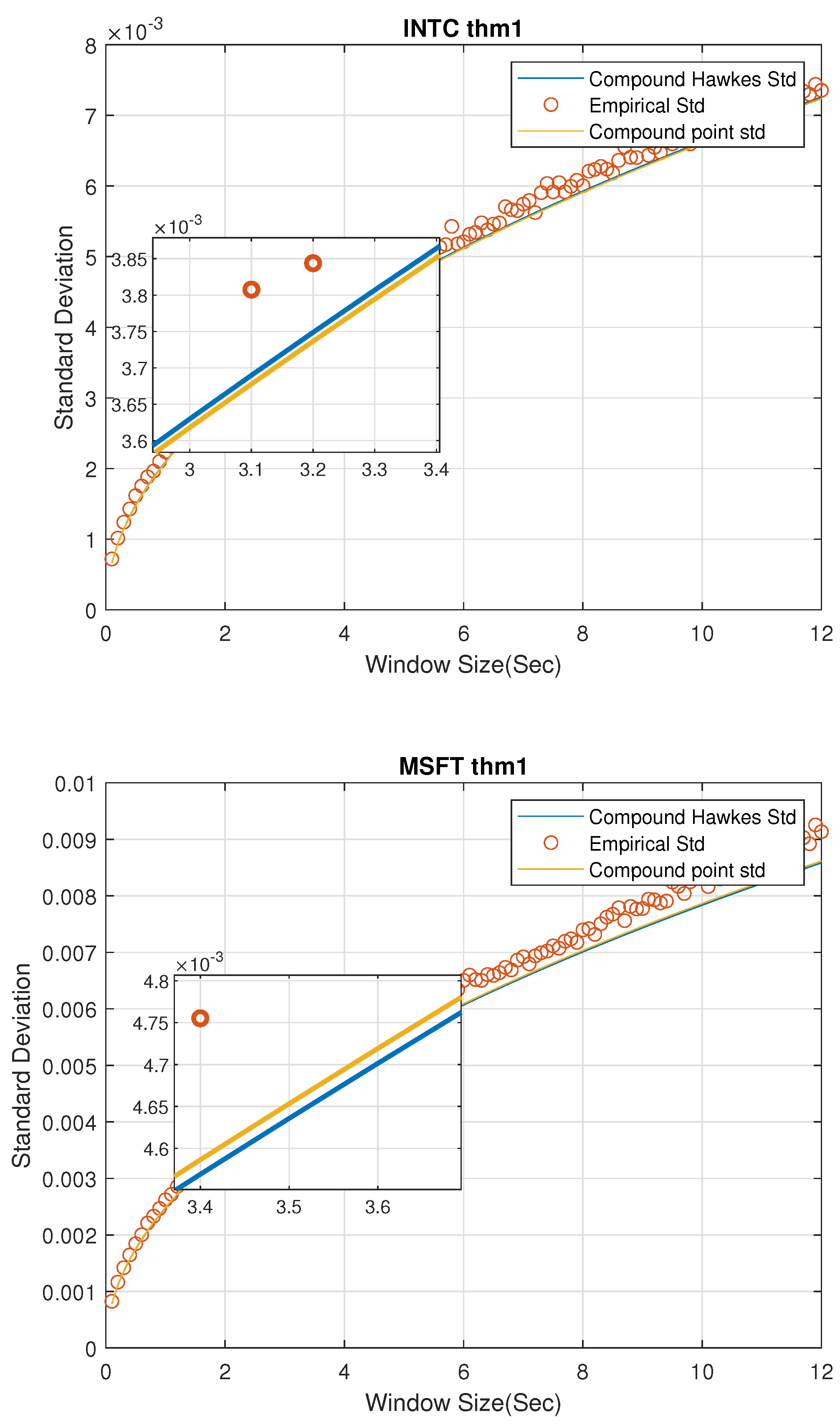
Figure 1 gives a standard deviation comparison of MGCPP, MGCHP, and the raw data for 2 stocks in different window sizes from 0.1 s to 12 s in steps of 0.1 s. First, we could find the MGCPP parameters make the standard deviation of LHS very similar to the RHS for each stocks when n is large. So, generally speaking, we can say our MGCPP model fits the data well. Second, the MGCPP curve is very close to the MGCHP curve or we could say the simulation results via Intel and Microsoft stocks data are nearly same. It shows that even we do not have a sophisticated intensity function as the Hawkes process, we still can reach a relative good result with a simple point process model. This can help us deal with the computing efficiency problem when using the MGCHP model. We’ll give more quantitative error analysis later.

Remark 7.

Since the number of windows decreases as the window size nt increases, we can find that the spread of data increases when the window size increases in Figure 1. For example, when we consider nt = 0.1 s, the number of windows is 234,000. However, a 12-s window size yields 1950 windows which will lead the standard deviation increases.

Intuitively, Figure 1 shows that the standard deviation of MGCHP and MGCPP are very close and both of them fit the real standard deviation very well. Next, we analyze MGCHP and MGCPP models quantitatively.

We computed the mean square error (MSE) of the real standard deviation and theoretical standard deviations in

Table 5. The mean square error (MSE) of the real standard deviation and theoretical standard deviations from MGCHP and MGCPP.

Ticker	MGCHP MSE	MGCPP MSE
INTC	$3.4039\times {10}^{-8}$	$3.9858\times {10}^{-8}$
MSFT	$9.6454\times {10}^{-8}$	$8.6189\times {10}^{-8}$

. As can be seen from Table 5, MGCHP model performs better than the MGCPP model with both Intel and Microsoft data. For Intel stock data, the MSE of MGCHP is 17% better than MGCPP and nearly 10% better than MGCPP model with the Microsoft stock data. However, when we compare the order of magnitude of the MSE (−8) with the real standard deviation (−2 and −3), we still can conclude that MGCPP is good enough for the mid-price modeling task.

Recall Equation (23), we can find the standard deviation and the square root of time step have a linear relationship. So, we can fit the real standard deviation data with the square root curve by using the least-square regression. Then, we can set the regression curve as a benchmark and compare the benchmark coefficients with two stochastic models.

From

Table 6. Coefficients calculated by MGCHP and MGCPP models. Benchmark coefficients are coefficients of the least-square regression curves. Percentage errors are differences between two stochastic models with the benchmark.

Ticker	MGCHP Coefficient	MGCPP Coefficient	Benchmark Coefficient	MGCHP % Error	MGCPP % Error
INTC	0.002086	0.002089	0.002162	$3.515\%$	$3.377\%$
MSFT	0.002494	0.002487	0.002609	$4.408\%$	$4.676\%$

, we can find that the percentage error of both two stochastic models are all smaller than 5% and there is no significant difference between the MGCPP coefficient and the MGCHP coefficient.

Based on the previous analysis, we can conclude that the empirical results of MGCHP and MGCPP are very close and all of them have a very good performance in the mid-price modeling. However, as for the MGCHP, we need to estimate many parameters. As the Guo and Swishchuk (2020) mentioned, if we consider a two-dimensional MGCHP (two stocks), we have to estimate 5 parameters for the Hawkes process part and the number of parameters increases dramatically to 55 when we consider a 5-dimensional case (5 stocks). The parameter estimation procedure is also quite time consuming for the MGCHP because of the complicated likelihood function of multivariate Hawkes process. For example, it takes a dozen hours to estimate parameters for a 3-dimensional Hawkes process (21 parameters) with LOBSTER data set by using the maximum likelihood estimation (MLE) and the particle swarm optimization (PSO) method in Guo and Swishchuk (2020). On the contrary, the number of parameters for MGCPP is much smaller than the MGCHP. In the two-dimensional case, we have 2 parameters to be estimated in the simple point process part and this increases to 5 parameters in the 5-dimensional case, which is much smaller than 55. The parameter estimation procedure is also quite simple and fast (in several seconds with the same data set) because we do not have to deal with the likelihood function. In this way, from the numerical perspective, the generalized model MGCPP is better than the MGCHP because of the fast and simple estimation procedure.

Remark 8.

Note that the numbers of parameters we mentioned before are all parameters of the order flow ${\overrightarrow{N}}_t$. Parameters of Markov chains for MGCHP and MGCPP are same.

In general, we showed that the results of the new generalized model are as good as the MGCHP and this kind of generalization has better numerical properties. In the following parts, we will explore the MGCPP model more.

3.3.3. MGCPP with $\mathcal{N}$-State Dependent Orders

We give more simulation examples by using the Google, Apple, and Amazon data with the MGCPP model with $\mathcal{N}$-state dependent orders in this section. Thanks to Swishchuk and Huffman (2020), we can conclude that the accuracy of the general compound Hawkes process model increases when the number of states increases. For Google, Apple, and Amazon in the LOBSTER data set, the best number of states is 4 to 7. In the previous section, we also showed that simulation results of MGCPP are nearly same as the MGCHP. So, it is reasonable to consider a MGCPP model with 7-state Markov chain here.

We applied the method in Swishchuk and Huffman (2020) to calculate the state values $a\left(X_{i,k}\right)$ for each stock. First, we compute the changes of mid-price and separate the data into two sets by positive increments or negative increments. Next, we calculate the quantiles for both data sets and split the data set according to the quantiles. If there are identical quantiles, we merge them into one. Then, we set the state values $a\left(X_{i,k}\right)$ as the average of mid-price changes located in each quantile (or merged quantile).

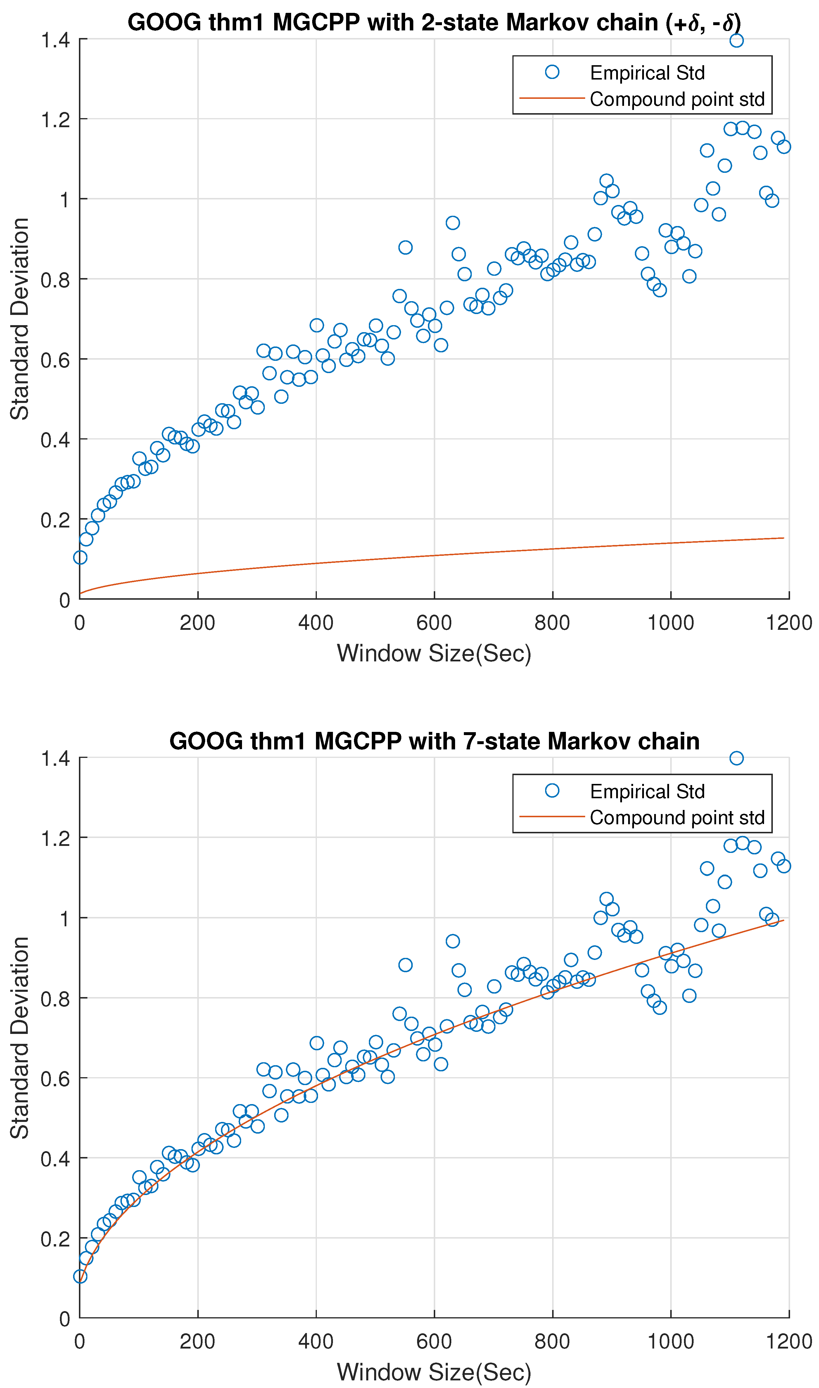
Figure 2, Figure 3 and Figure 4 give standard deviation comparisons for MGCPP with 2-state Markov chain and 7-state Markov chain simulated by different tickers’ data. Since the 2-state simulation results here are not as good as the results simulated by Intel’s and Microsoft’s data, we take bigger time steps and window sizes (from 10 s to 20 min with 10 s time step) to capture more dynamics. From figures we can find that the 7-state model has a significant improvement than the 2-state model. Seven-state curves for AAPL and GOOG are very close to the real standard deviation, although the theoretical curve of AMZN is underestimated even with the 7-state model.

Table 7. The MSE and coefficients computed by MGCPP with 2-state and 7-state Markov chain for different tickers. The regression coefficients were derived by fitting the real standard deviations with square root curve. The MGCPP coefficients were computed by Equation (23).

Ticker	MSE	Regression Ceofficient	MGCPP Ceofficient	Percentage Error
AAPL 2-state	0.2467	0.0278	0.0076	72.66%
AAPL 7-state	0.0064	0.0311	0.0288	7.40%
GOOG 2-state	0.4161	0.0307	0.0044	85.67%
GOOG 7-state	0.0081	0.0307	0.0287	6.51%
AMZN 2-state	0.1233	0.0189	0.0048	74.60%
AMZN 7-state	0.0225	0.0205	0.0147	28.29%

lists the MSE and coefficients of the 2-state and 7-state models with different tickers. We can find the improvement of 7-state model quantitatively from the table. The results of AAPL and GOOG are good enough for the mid-price modeling. As for AMZN, although we derive a remarkable improvement from 2-state model (74.60% error) to 7-state model (28.29% error), we cannot make the error smaller than 5% or 10%. This is to say, MGCPP model may not be able to capture the full dynamics for AMZN data, but it still can be a strong candidate for modeling the mid-price, which is consistent with the conclusion of compound Hawkes model in Swishchuk and Huffman (2020).

Remark 9.

The MGCPP is not only a generalization of MGCHP, but also a generalization for all multivariate compound models whose point processes $\overrightarrow{N_t}$ satisfy the Assumptions 1 and 2. The reason we use Hawkes process for comparison is we want to take the advantage of numerical examples in references.

4. Diffusion Limit for the MGCPP: Deterministic Centralization

We proved a LLN and FCLT for the MGCPP in the previous section. Limit theorems provide us an approximation for the mid-price modeling in the LOB. Recall the approximation in Remark 5, we have

$${\overrightarrow{S}}_{nt}\sim {\tilde{\sigma }}^{*}{\Lambda }^{1/2}\overrightarrow{W}\left(t\right)\sqrt{n}+\widetilde{a^{*}}{\overrightarrow{N}}_{nt},$$

(24)

where the ${\overrightarrow{S}}_{nt}$ is the price process and ${\overrightarrow{N}}_{nt}$ is the order flow. However, in the real-world problems, Equation (24) cannot help us with the forecasting task directly because we cannot observe the future order flow ${\overrightarrow{N}}_{nt}$ in advance. This is the motivation for us to consider a FCLT II for the MGCPP model.

4.1. FCLT for MGCPP: Deterministic Centralization

Theorem 3.

(FCLT II: Deterministic Centralization). Let $X_{i,k},i=1,2,\cdots ,d$ be independent ergodic Markov chains defined before. $X^{\left\{i\right\}}=\{1,2,\cdots ,{\mathcal{N}}_i\}$ is the state space and the ergodic probabilities is given by $\left({\pi }_{i,1}^{*},{\pi }_{i,2}^{*},\dots ,{\pi }_{i,n}^{*}\right)$. Assume $X_{i,k}$ is independent of ${\overrightarrow{N}}_t$. Let ${\overrightarrow{S}}_{nt}$ be d-dimensional MGCPP, we have

$$\frac{{\overrightarrow{S}}_{nt}-\widetilde{a^{*}}E\left({\overrightarrow{N}}_{nt}\right)}{\sqrt{n}}\stackrel{n\to \infty }{\to }{\tilde{\sigma }}^{*}{\Lambda }^{1/2}{\overrightarrow{W}}_1\left(t\right)+\widetilde{a^{*}}{\Sigma }^{1/2}{\overrightarrow{W}}_2\left(t\right),forallt>0,$$

(25)

where ${\overrightarrow{W}}_1\left(t\right)$ and ${\overrightarrow{W}}_2\left(t\right)$ are independent d-dimensional Brownian motions. Parameters ${\tilde{\sigma }}^{*}$, $\stackrel{\Sigma }{a^{*}}$, Λ, and Σ are defined in Theorem 2.

Proof of Theorem 3.

Recall the FCLT for MPP (Assumption 2), we have

$$\left(\frac{1}{\sqrt{n}}{\overrightarrow{N}}_{nt}-\frac{1}{\sqrt{n}}E\left({\overrightarrow{N}}_{nt}\right)\right)\stackrel{n\to \infty }{\to }{\Sigma }^{1/2}{\overrightarrow{W}}_t$$

(26)

in law for the Skorokhod topology. From Theorem 2, we have the FCLT for MGCPP

$$\frac{{\overrightarrow{S}}_{nt}-\widetilde{a^{*}}{\overrightarrow{N}}_{nt}}{\sqrt{n}}\stackrel{n\to \infty }{\to }{\tilde{\sigma }}^{*}{\Lambda }^{1/2}{\overrightarrow{W}}_t,forallt>0$$

(27)

in the weak law of Skorokhod topology. Here, we assume two multivariate Brownian motions in (26) and (27) are mutually independent and we refer them ${\overrightarrow{W}}_2\left(t\right)$ and ${\overrightarrow{W}}_1\left(t\right)$. Let ${\mathcal{G}}_t$ be the $\sigma$-algebra generated by $N_i\left(s\right)$, $s\le t$, $1\le i\le d$. Since ${\overrightarrow{N}}_t$ and the Markov chain $a\left(X_{i,k}\right)$ are independent, ${\overrightarrow{S}}_t$ is only determined by ${\overrightarrow{N}}_t$ and $a\left(X_{i,k}\right)$, we can have processes

$$\left(\frac{1}{\sqrt{n}}{\overrightarrow{N}}_{nt}-\frac{1}{\sqrt{n}}E\left({\overrightarrow{N}}_{nt}\right)\right),$$

(28)

and

$$\frac{{\overrightarrow{S}}_{nt}-\widetilde{a^{*}}{\overrightarrow{N}}_{nt}}{\sqrt{n}}$$

(29)

are ${\mathcal{G}}_t$-conditional independent. Similar to the central limit theorem in Prakasa-Rao (2009), we consider the convergence of conditional expectations for processes (28) and (29) on ${\mathcal{G}}_t$. Then with the characteristic functions for both limiting processes, we have the joint convergence

$$\left(\frac{1}{\sqrt{n}}{\overrightarrow{N}}_{nt}-\frac{1}{\sqrt{n}}E\left({\overrightarrow{N}}_{nt}\right),\frac{{\overrightarrow{S}}_{nt}-{\tilde{a}}^{*}{\overrightarrow{N}}_{nt}}{\sqrt{n}}\right)\stackrel{\mathrm{conditional}\mathrm{on}{\mathcal{G}}_t}{\to }\left({\Sigma }^{1/2}{\overrightarrow{W}}_2\left(t\right),{\tilde{\sigma }}^{*}{\Lambda }^{1/2}{\overrightarrow{W}}_1\left(t\right)\right)$$

(30)

as $n\to \infty$. Next, consider

$$\frac{{\overrightarrow{S}}_{nt}}{\sqrt{n}}-\frac{{\tilde{a}}^{*}E({\overrightarrow{N}}_{nt})}{\sqrt{n}}=\frac{{\overrightarrow{S}}_{nt}-{\tilde{a}}^{*}{\overrightarrow{N}}_{nt}}{\sqrt{n}}+{\tilde{a}}^{*}\left(\frac{1}{\sqrt{n}}{\overrightarrow{N}}_{nt}-\frac{1}{\sqrt{n}}E({\overrightarrow{N}}_{nt})\right).$$

(31)

By (30) we can derive

$$\frac{{\overrightarrow{S}}_{nt}-{\tilde{a}}^{*}{\overrightarrow{N}}_{nt}}{\sqrt{n}}+{\tilde{a}}^{*}\left(\frac{1}{\sqrt{n}}{\overrightarrow{N}}_{nt}-\frac{1}{\sqrt{n}}E\left({\overrightarrow{N}}_{nt}\right)\right)⟶{\tilde{\sigma }}^{*}{\Lambda }^{1/2}{\overrightarrow{W}}_1\left(t\right)+\widetilde{a^{*}}{\Sigma }^{1/2}{\overrightarrow{W}}_2\left(t\right)$$

(32)

as $n\to \infty$ which gives (25). ☐

Remark 10.

We can also consider a special case as the FCLT I. Let $X_{i,k}$ be a Markov chain with two dependent states $(+\delta ,-\delta )$ and the ergodic probabilities are $\left({\pi }_i^{*},1-{\pi }_i^{*}\right)$. Set $a_i\left(x\right)=(-\delta )\vee (x\wedge \delta )$ in the Definition 7. Then, we can derive a similar result for FCLT II. Parameters ${\tilde{a}}^{*}$ and ${\tilde{\sigma }}^{*}$ can be computed by Equation (19).

Remark 11.

For the FCLT II, we can also consider a similar approximation as the FCLT I. For some large enough n, we have

$${\overrightarrow{S}}_{nt}\sim \sqrt{n}{\tilde{\sigma }}^{*}{\Lambda }^{1/2}{\overrightarrow{W}}_1\left(t\right)+\sqrt{n}\widetilde{a^{*}}{\Sigma }^{1/2}{\overrightarrow{W}}_2\left(t\right)+\widetilde{a^{*}}E\left({\overrightarrow{N}}_{nt}\right),forallt>0.$$

(33)

To deal with the $E({\overrightarrow{N}}_{nt})$ term, we consider the approximation derived from Assumption 1 in Equation (22):

$$E(\overrightarrow{N}\left(nt\right))\sim nt\overrightarrow{\overline{\lambda }}.$$

(34)

Rewrite Equation (33), we have the new approximation

$${\overrightarrow{S}}_{nt}\sim \sqrt{n}{\tilde{\sigma }}^{*}{\Lambda }^{1/2}{\overrightarrow{W}}_1\left(t\right)+\sqrt{n}\widetilde{a^{*}}{\Sigma }^{1/2}{\overrightarrow{W}}_2\left(t\right)+\widetilde{a^{*}}nt\overrightarrow{\overline{\lambda }}.$$

(35)

4.2. Numerical Examples for FCLT: Deterministic Centralization

In this Section, we applied the LOBSTER data to test the FCLT II. According to the numerical examples of FCLT I, we consider the standard deviation of the approximation in Remark 11, namely

$$std\left\{{\overrightarrow{S}}_{(i+1)nt}-{\overrightarrow{S}}_{int}\right\}\approx \sqrt{{\left({\tilde{\sigma }}^{*}\right)}^2\Lambda n\overrightarrow{t}+{\left(\widetilde{a^{*}}\right)}^2\Sigma n\overrightarrow{t}}.$$

(36)

First, we estimated the covariance matrix Σ by applying the Assumption 2. When n is large enough, have the approximation:

$$\frac{1}{\sqrt{n}}({\overrightarrow{N}}_{nt}-E\left({\overrightarrow{N}}_{nt}\right))\sim {\Sigma }^{1/2}{\overrightarrow{W}}_t,t\in [0,1].$$

(37)

Take the covariance for both side of (37), we have

$$\frac{1}{nt}\left(\mathrm{Cov}(N_i\left(nt\right),N_j\left(nt\right))\right)\sim {\Sigma }_{i,j},t\in [0,1],i,j=1,2,\cdots ,d.$$

(38)

Then, we can derive the estimated Σ for 5 stocks in

Table 8. Estimated covariance matrix $\Sigma$ of 5 stocks via the FCLT assumption.

Ticker	INTC	MSFT	AAPL	AMZN	GOOG
INTC	0.4844	0.1719	1.2393	0.5317	0.5312
MSFT	0.1719	0.5634	1.8361	0.7834	0.7162
AAPL	1.2393	1.8361	62.3800	6.7811	6.4331
AMZN	0.5317	0.7834	6.7811	19.2883	1.9617
GOOG	0.5312	0.7162	6.4331	1.9617	22.7980

.

Comparisons of real standard deviation and theoretical standard deviation can be found in Figure 5. Since results of INTC and MSFT are good enough with the 2-state Markov chain $(+\delta ,-\delta )$ in FCLT I, we also applied 2-state Markov chain for INTC and MSFT here. As for AAPL, GOOG, and AMZN, we used the MGCPP model with 7-state Markov chain. Window sizes here start from 1 s and increase to 20 min in time steps of 10 s. As can be seen in Figure 5, the results for FCLT II are as good as the FCLT I results in Figure 1, Figure 2, Figure 3 and Figure 4. We also computed the MSE and coefficients in

Table 9. The MSE and coefficients computed by MGCPP FCLT II.

Ticker	MSE	Benchmark Ceofficient	MGCPP Ceofficient	Percentage Error
INTC 2-state	1.4452 × ${10}^{-5}$	2.2361 × ${10}^{-3}$	2.0958 × ${10}^{-3}$	6.27%
MSFT 2-state	6.6227 × ${10}^{-5}$	2.5157 × ${10}^{-3}$	2.4919 × ${10}^{-3}$	0.94%
AAPL 7-state	6.1382 × ${10}^{-3}$	2.7799 × ${10}^{-2}$	2.8788 × ${10}^{-2}$	3.56%
GOOG 7-state	8.0981 × ${10}^{-3}$	3.0736 × ${10}^{-2}$	2.8686 × ${10}^{-2}$	6.67%
AMZN 7-state	1.1156 × ${10}^{-2}$	1.8940 × ${10}^{-2}$	1.4747 × ${10}^{-2}$	22.14%
Overall Percentage Error	7.92%

. Benchmark coefficients are from the least-square regression curves which are similar as benchmarks in Table 6.

We see that the percentage errors of MSFT and AAPL are very small (less than $5\%$) and the results of INTC and GOOG are also good (less than $10\%$). The percentage error of AMZN is large, but it is still smaller than the error derived from FCLT I in Table 7. In general, the simulation results of FCLT II is as good as the FCLT I and we can apply this FCLT II to model a mid-price.

4.3. Rolling Cross-Validation

In this section, we tested the forecast ability of the MGCPP model. Since we did not assume the multivariate point process ${\overrightarrow{N}}_t$ is stationary, we cannot apply the K-fold cross-validation directly. Here, we used the rolling K-fold cross-validation method which proposed in Bergmeir et al. (2018). We divided the last 50 mins’ data into 5 disjoint 10-min windows for each stock. For the fold 1, We take the first 280 mins’ data as the training set to estimate parameters. Then, we applied the data in the next 10-min window to calculate the percentage error. Next, we merge the test set into the training set in fold 1 as the new training set in fold 2 and apply the next 10-min window as a new test set. Repeating this procedure 5 times, we will get 5 percentage errors. The mean value of the 5 percentage errors will be the test error E for this stock. So, the overall test error for our multivariate model is the average of all test errors. Figure 6 gives an example diagram for the rolling cross-validation.

Table 10. Test Errors for different tickers by applying 5-fold cross-validation. The errors are percentage errors between benchmark coefficients and the MGCPP coefficients.

Ticker	Fold 1	Fold 2	Fold 3	Fold 4	Fold 5	Mean Error
INTC	6.75%	0.39%	3.16%	14.32%	16.60%	8.24%
MSFT	20.33%	31.35%	16.96%	8.33%	22.61%	19.92%
AAPL	8.22%	0.51%	22.53%	21.34%	23.33%	15.01%
GOOG	19.60%	20.41%	16.41%	6.13%	12.51%	15.19%
AMZN	20.78%	4.87%	7.98%	18.81%	42.15%	18.92%
Overall Test Error	$E_{test}=15.46\%$

lists test errors for different tickers and the overall test error for the MGCPP model. As can be seen from the table, the test error for each stock is relatively large and the overall test error (15.46%) is nearly double the overall percentage error (7.92%) in Table 9. That is because the results in Table 9 is a fitting error while the test errors in Table 10 is a kind of forecast error. We did not apply any future information when we conduct the forecast task. So, even the 15.46% overall test error is not as good as the fitting one, it is still a good prediction in the LOB and can provide lots of insights in the forecast task.

5. Conclusions and Future Work

In this paper, we proposed a MGCPP model for the mid-price modeling in limit order book. This kind of process is a generalization of several stochastic models in the limit order market. We applied LOBSTER data to conduct simulations and found the multivariate generalized model is as good as the general compound Hawkes process model. We also tested the prediction ability of this kind of process. In general, the MGCPP performs very well in LOB modeling and it can be a meaningful reference in the mid-price prediction. In the future, we will explore more applications of the MGCPP and consider related option pricing problems under this kind of frame work.

References

1. Bacry, Emmanuel, Sylvain Delattre, Marc Hoffmann, and Jean-François Muzy. 2013. Some limit theorems for Hawkes processes and application to financial statistics. Stochastic Processes and Their Applications 123: 2475–99. [Google Scholar] [CrossRef]
2. Bowsher, Clive G. 2007. Modelling security market events in continuous time: Intensity based, multivariate point process models. Journal of Econometrics 141: 876–912. [Google Scholar] [CrossRef] [Green Version]
3. Brémaud, Pierre, and Laurent Massoulié. 1996. Stability of nonlinear Hawkes processes. The Annals of Probability 1: 1563–88. [Google Scholar]
4. Bjork, Tomas. 2011. Introduction to Point Processes from a Martingale Point of View. Stockholm: KTH. [Google Scholar]
5. Bauwens, Luc, and Nikolaus Hautsch. 2009. Modelling Financial High Frequency Data Using Point Processes. Berlin/Heidelberg: Springer. [Google Scholar]
6. Bergmeir, Christoph, Rob J. Hyndman, and Bonsoo Koo. 2018. A note on the validity of cross-validation for evaluating autoregressive time series prediction. Computational Statistics and Data Analysis 120: 70–83. [Google Scholar] [CrossRef]
7. Cartea, Álvaro, Sebastian Jaimungal, and José Penalva. 2015. Algorithmic and High-Frequency Trading. Cambridge: Cambridge University Press. [Google Scholar]
8. Chen, Shizhe, Ali Shojaie, Eric Shea-Brown, and Daniela Witten. 2019. The Multivariate Hawkes Process in High Dimensions: Beyond Mutual Excitation. arXiv arXiv:1707.04928v2. [Google Scholar]
9. Cont, Rama, and Adrien De Larrard. 2013. Price dynamics in a Markovian limit order market. SIAM Journal on Financial Mathematics 4: 1–25. [Google Scholar] [CrossRef] [Green Version]
10. Embrechts, Paul, Thomas Liniger, and Lu Lin. 2011. Multivariate Hawkes processes: An application to financial data. Journal of Applied Probability 48: 367–78. [Google Scholar] [CrossRef] [Green Version]
11. Guo, Qi, and Anatoliy Swishchuk. 2020. Multivariate general compound Hawkes processes and their applications in limit order books. Wilmott 107: 42–51. [Google Scholar] [CrossRef]
12. Lemonnier, Rémi, Kevin Scaman, and Argyris Kalogeratos. 2017. Multivariate Hawkes Processes for Large-Scale Inference. Paper presented at Thirty-First AAAI Conference on Artificial Intelligence, San Francisco, CA, USA, February 4–9. [Google Scholar]
13. Liniger, Thomas Josef. 2009. Multivariate Hawkes Processes. Ph.D. dissertation, Swiss Federal Institute of Technology in Zurich, Zurich, Switzerland. [Google Scholar]
14. Norris, James R. 1998. Markov Chains. Cambridge: Cambridge University Press. [Google Scholar]
15. Rao, B. L. S. Prakasa. 2009. Conditional independence, conditional mixing and conditional association. Annals of the Institute of Statistical Mathematics 61: 441–60. [Google Scholar]
16. Swishchuk, Anatoliy. 2017. Risk model based on compound Hawkes process. Wilmott 94: 50–57. [Google Scholar]
17. Swishchuk, Anatoliy, and Nelson Vadori. 2017. A semi-Markovian modelling of limit order markets. SIAM Journal on Financial Mathematics 8: 240–73. [Google Scholar] [CrossRef] [Green Version]
18. Swishchuk, Anatoliy, Tyler Hofmeister, Katharina Cera, and Julia Schmidt. 2017. General semi-Markov model for limit order books. International Journal of Theoretical and Applied Finance 20: 1750019. [Google Scholar] [CrossRef]
19. Swishchuk, Anatoliy, and Aiden Huffman. 2020. General compound Hawkes processes in limit order books. Risks 8: 28. [Google Scholar] [CrossRef] [Green Version]
20. Vinkovskaya, Ekaterina. 2014. A Point Process Model for the Dynamics of LOB. Ph.D. dissertation, Columbia University, New York, NY, USA. [Google Scholar]
21. Vadori, Nelson, and Anatoliy Swishchuk. 2015. Strong law of large numbers and central limit theorems for functionals of inhomogeneous Semi-Markov processes. Stochastic Analysis and Applications 33: 213–43. [Google Scholar] [CrossRef]
22. Yang, Yingxiang, Jalal Etesami, Niao He, and Negar Kiyavash. 2017. Online Learning for Multivariate Hawkes Processes. Paper presented at 31st Conference on Neural Information Processing Systems, Long Beach, CA, USA, December 4–9. [Google Scholar]
23. Zheng, Ban, François Roueff, and Frédéric Abergel. 2014. Ergodicity and scaling limit of a constrained multivariate Hawkes process. SIAM Journal on Financial Mathematics 5: 99–136. [Google Scholar] [CrossRef]
24. Zhu, Lingjiong. 2013. Central limit theorem for nonlinear Hawkes processes. Journal of Applied Probability 50: 760–71. [Google Scholar] [CrossRef]
Figure 1. Standard deviation comparisons for 2 stocks by FCLT I for multivariate general compound point process (MGCPP) and multivariate general compound Hawkes process (MGCHP).
Risks 08 00098 g001
Figure 2. Standard deviation comparisons for MGCPP with 2-state Markov chain and 7-state Markov chain simulated by Apple’s stock data.
Risks 08 00098 g002
Figure 3. Standard deviation comparisons for MGCPP with 2-state Markov chain and 7-state Markov chain simulated by Google’s stock data.
Risks 08 00098 g003
Figure 4. Standard deviation comparisons for MGCPP with 2-state Markov chain and 7-state Markov chain simulated by Amazon’s stock data.
Risks 08 00098 g004
Figure 5. Standard deviation comparisons for 5 stocks by FCLT II for the MGCPP. INTC and MSFT are simulated with 2-state Markov chain while AAPL, AMZN, and GOOG are using 7-state Markov chain.
Risks 08 00098 g005
Figure 6. Diagram for the Rolling cross-validation.
Risks 08 00098 g006