1. Introduction
A non-life insurance company faces premium risk, among others, which is the risk of financial losses related to premiums earned. The risk in the losses relates to uncertainty in severity, frequency or even timing of claims incurring during the period of exposure. For an operating non-life insurer, premium risk is a key driver of uncertainty both from operational and solvency perspectives. In regards to the solvency perspective, there are many different methods useful to give a correct view of the capital needed to meet adverse outcomes related to premium risk. In particular, evaluation of the distribution of aggregate loss plays a fundamental role in the analysis of risk and solvency levels.
As shown in
Cerchiara and Demarco (
2016), the standard formula under Solvency II for premium and reserve risk defined by the Delegated Acts (DA, see
European Commission 2015) proposes the following formula for the solvency capital requirement (SCR):
where
V denotes the net reinsurance volume measure for Non-Life premium and reserve risk determined in accordance with Article 116 of DA, and
is the volatility (coefficient of variation) for Non-Life premium and reserve risk determined in accordance with Article 117 of DA, combining the volatility
according to the correlation matrix between each segment
s. Then,
is calculated as follows:
In this paper we focus our attention on
, i.e., the coefficient of variation of the Fire segment Premium Risk. Under DA, the premium risk volatility of this segment is equal to 8%. As shown in
Clemente and Savelli (
2017), Equation (
1) “implicitily assumes to measure the difference between the Value at Risk (VaR) at 99.5% confidence level and the mean of the probability distribution of aggregate claims amount by using a fixed multiplier of the volatility equal to 3 for all insurers. From a practical point of view, DA multiplier does not take into account the skewness of the distribution with a potential underestimation of capital requirement for small insurers and an overestimation for big insurers”.
For Insurance Undertakings who do not believe in the standard formula assumptions, they may calculate the Solvency Capital Requirement using an Undertaking Specific Parameters approach (USP, see
Cerchiara and Demarco 2016) and a Full or Partial Internal Model (PIM) after approval by Supervisory Authorities. Calculation of the volatility and VaR of independent or dependent risky positions using PIM is very difficult for large portfolios. In the literature, many different studies are based on definitions of composite models that aim to analyze loss distribution and dependence between the main factors that characterize the risk profile of insurance companies, e.g., frequency and severity, attritional and large claims and so forth. Considering more recent developments in the literature,
Galeotti (
2015) proves the convergence of a geometric algorithm (alternative to Monte Carlo and quasi-Monte Carlo methods) for computing the Value-at-Risk of a portfolio of any dimension, i.e., the distribution of the sum of its components, which can exhibit any dependence structure.
In order to implement PIM and investigate overestimation of the SCR (and the underlying volatility) for large insurers, we used the Danish fire insurance dataset
1 that has been often analyzed according to the parametric approach and composite models.
McNeil (
1997),
Resnick (
1997),
Embrechts et al. (
1997) and
McNeil et al. (
2005) proposed fitting this dataset using Extreme Value Theory and Copula Functions (see
Klugman et al. 2010 for more details on the latter), with special reference to modeling the tail of the distribution.
Cooray and Ananda (
2005) and
Scollnik (
2007) showed that the composite lognormal-Pareto model was a better fit than standard univariate models. Following the previous two papers,
Teodorescu and Vernic (
2009,
2013) fit the dataset firstly with a composite Exponential and Pareto distribution, and then with a more general composite Pareto model obtained by replacing the Lognormal distribution by an arbitrary continuous distribution, while
Pigeon and Denuit (
2011) considered a positive random variable as the threshold value in the composite model. There have been several other approaches to model this dataset, including Burr distribution for claim severity using XploRe computing environment (
Burnecki and Weron 2004), Bayesian estimation of finite time ruin probabilities (
Ausin et al. 2009), hybrid Pareto models (
Carreau and Bengio 2009), beta kernel quantile estimation (
Charpentier and Oulidi 2010) and bivariate composite Poisson process (
Esmaeili and Klüppelberg 2010). An example of non-parametric modeling is shown in
Guillotte et al. (
2011) with a Bayesian inference on bivariate extremes.
Drees and Müller (
2008) showed how to model dependence within joint tail regions.
Nadarajah and Bakar (
2014) improved the fittings for the Danish fire insurance data using various new composite models, including the composite Lognormal–Burr model.
Following this literature, this paper innovates fitting of the Danish fire insurance data by using the
Pigeon and Denuit (
2011) composite model with a random threshold that has a higher goodness-of-fit than the
Nadarajah and Bakar (
2014) model. Once the best model is defined, we show that the Standard formula assumption is prudent, especially for large insurance companies, giving an overestimated volatility of the premium risk (and of the SCR). For illustrative purposes, we also investigate the use of other models, including the Copula function and Fast Fourier Transform (FFT;
Robe-Voinea and Vernic 2016), trying to take into account the dependence between attritional and large claims and understand the effect on SCR.
The paper is organized as follows. In
Section 2 we report some statistical characteristics of Danish data. In
Section 3 and
Section 4 we posit there is no dependence between attritional and large claims. We investigate the use of composite models with fixed or random thresholds in order to fit the Danish fire insurance data, and we compare our numerical results with the fitting of
Nadarajah and Bakar (
2014) based on a composite Lognormal–Burr model. In
Section 5 we try to appraise risk dependence through the Copula function concept and FFT, for which
Robe-Voinea and Vernic (
2016) provide an overview and perform a multidimensional application.
Section 6 concludes the work and presents estimation of the aggregate loss volatility distribution, and results are compared under independence and dependence conditions.
2. Data
In the following, we show some statistics of the dataset used in this analysis. The losses of individual fires covered in Denmark were registered by the reinsurance company Copenhagen Re and, for our study, have been converted into euros. It is worth mentioning that the original dataset (available also in R) covers the period 1980–1990. In 2003–2004, Mette Havning (Chief Actuary of Danish Reinsurance) was on the Astin committee where she met Tine Aabye from Forsikring & Pension. Aabye asked her colleague to send the Danish million re-losses from 1985–2002 to Mette Havning. Based on the two versions from 1980–1990 and 1985–2002, Havning then made an extended version of Danish Fire Insurance Data from 1980 through 2002 with only a few ambiguities in the overlapping period. The data were communicated to us by Mette Havning and consisted of 6870 claims over a time period of 23 years. We bring to the reader’s attention that, to avoid seasonal effects due to the use of the entire historical series that starts from 1980, the costs have been inflated to 2002. In addition, we referred to a wider dataset also including small losses, unlike that used by
McNeil (
1997), among others. In fact, we want to study the entire distribution of this dataset, while in
McNeil (
1997) and in other works the attention was focused especially on the right-tail distribution. We list some descriptive statistics in
Table 1:
The maximum observed was around €55 million and the average cost was 613,100€. The empirical distribution is definitely leptokurtic and asymmetric to the right.
To make applications of composite models and Copula functions easier, we will suppose that claim frequency
k is non-random, while for the Fast Fourier Transform algorithm we consider the frequency as a random variable. The losses have been split by year, so we can report some descriptive statistics for
k in
Table 2:
We note 50% of frequencies were included between 238 and 381 claims, and there is slight negative asymmetry. In addition, the variance is greater than mean value (299).
3. Composite Models
In the Danish fire insurance data we can find both frequent claims with low to medium severity and sporadic claims with high severity. If we want to define a joint distribution for these two types of claims we have to build a composite model.
A composite model is a combination of two different models: One having a light tail below a threshold (attritional claims) and another with a heavy tail suitable to model the value that exceeds this threshold (large claims). Composite distributions (also known as composite, spliced or piecewise distributions) have been introduced in many applications.
Klugman et al. (
2010) expressed the probability density function of a composite distributions as
where
is truncated probability density function of marginal distribution
,
;
are mixing weights,
; and
defines the range limit of the domain.
Formally, the density distribution of a composite model can be written as a special case of (
3) as follows:
where
, and
and
are cut off density distributions of marginals
and
, respectively. In detail, if
is the distribution function of
, then we have
It is simple to note that (
4) is a convex combination of
and
with weights
r and
. In addition, we want (
4) to be continuous, derivable and with a continuously derivative density function, and for this scope we fix the following limitation:
From the first we obtain
while from the second
We can define distribution function
F of (
4)
Suppose
and
admit inverse functions; we can define the quantile function via an inversion method. Let
p be a random number from a standard Uniform distribution, then the quantile function results in
To estimate the parameters of (
9) we can proceed as follows: First, we estimate marginal density function parameters separately (the underlying hypothesis is that there is no relation between attritional and large claims); then, these estimates will be the start values of the density function in order to maximize the following likelihood:
where
n is the sample dimension,
is a vector including composite model parameters, while
m is such that
, otherwise
m is the level of order statistics
immediately previous (or coincident) to
u.
The methodology described in
Teodorescu and Vernic (
2009,
2013) has been used in order to estimate threshold
u, which permits us to discriminate between attritional and large claims.
3.1. Composite Model with Random Threshold
We can define a composite model also using a random threshold (see
Pigeon and Denuit 2011). In particular, given a random sample
, we can assume that every single component
provides its own threshold. So, for the generic observation
we will have the threshold
,
. For this reason,
are realizations of a random variable
U with a distribution function G. The random variable
U is necessarily non-negative and with a heavy-tailed distribution.
A composite model with a random threshold shows a completely new and original aspect: Not only are we unable to choose a value for u, but its whole distribution and the parameters of the latter are implicit in the definition of the composite model. In particular, we define the density function of the Lognormal–Generalized Pareto Distribution model (GPD, see (
Embrechts et al. 1997)) with a random threshold in the following way:
where
,
U is the random threshold with density function
g,
and
are Lognormal and GPD density functions, respectively,
is the Standard Normal distribution function,
is the shape parameter of GPD and
is the Lognormal scale parameter.
3.2. Kumaraswamy Distribution and some Generalization
In this section we describe the Kumaraswamy Distribution (see
Kumaraswamy 1980) and a generalization of the Gumbel distribution (see
Cordeiro et al. 2012). In particular, let
in the distribution proposed in
Kumaraswamy (
1980), where
and
are non-negative shape parameters. If G is the distribution function of a random variable, then we can define a new distribution by
where
and
are shape parameters that influence kurtosis and skewness. The Kumaraswamy–Gumbel (KumGum) distribution is defined throughout (
14) with the following distribution function (see
Cordeiro et al. 2012):
where
is the Gumbel distribution function with density defined by (
20). The quantile function of KumGum is obtained by inverting (
15) and explicating Gumbel parameters (
v and
):
with
.
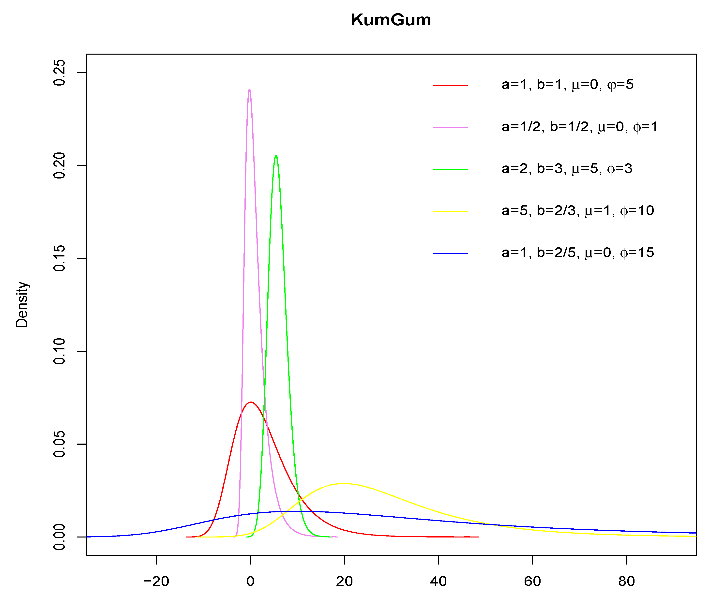
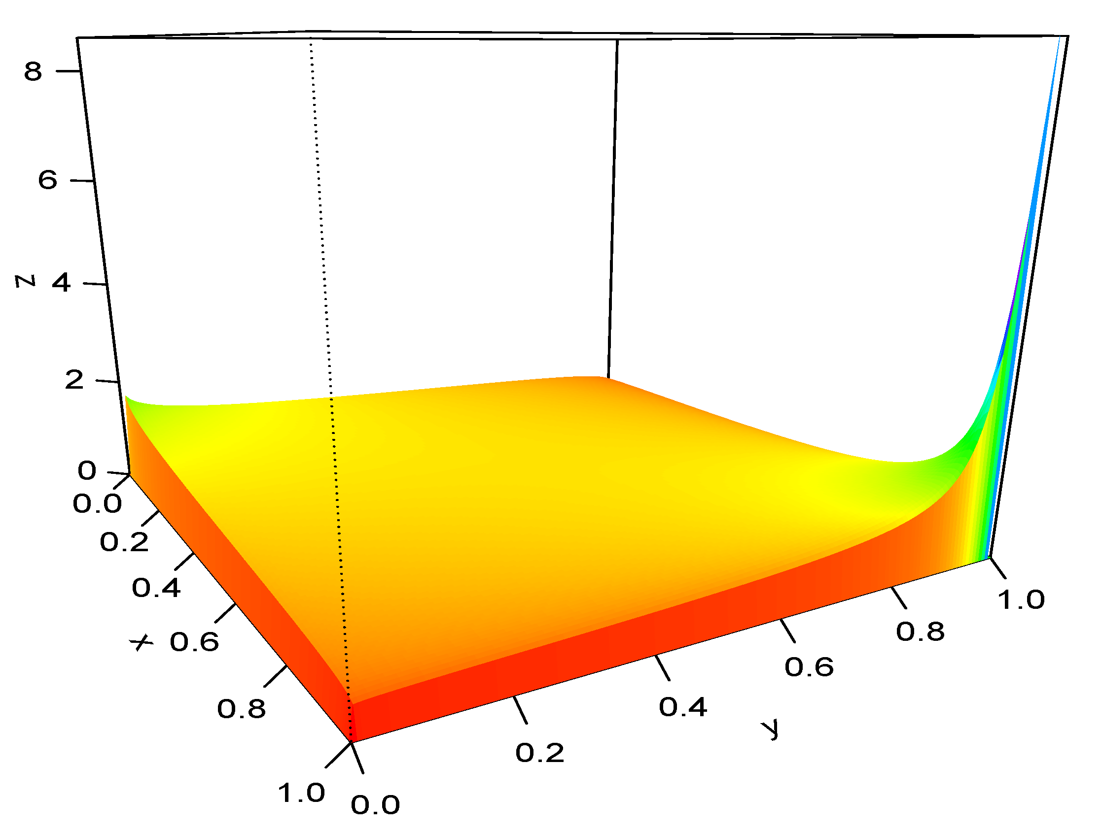
The following
Table 3 and
Figure 1 show the Kurtosis and Skewness of the KumGum density function by varying the four parameters:
Another generalization of the Kum distribution is the Kumaraswamy–Pareto one (KumPareto). In particular, we can evaluate Equation (
14) in the Pareto distribution function
P which is
where
is a scale parameter, and
is a shape parameter. Thus, from (
13), (
14) and (
17) we obtain the KumPareto distribution function:
The corresponding quantile function is
where
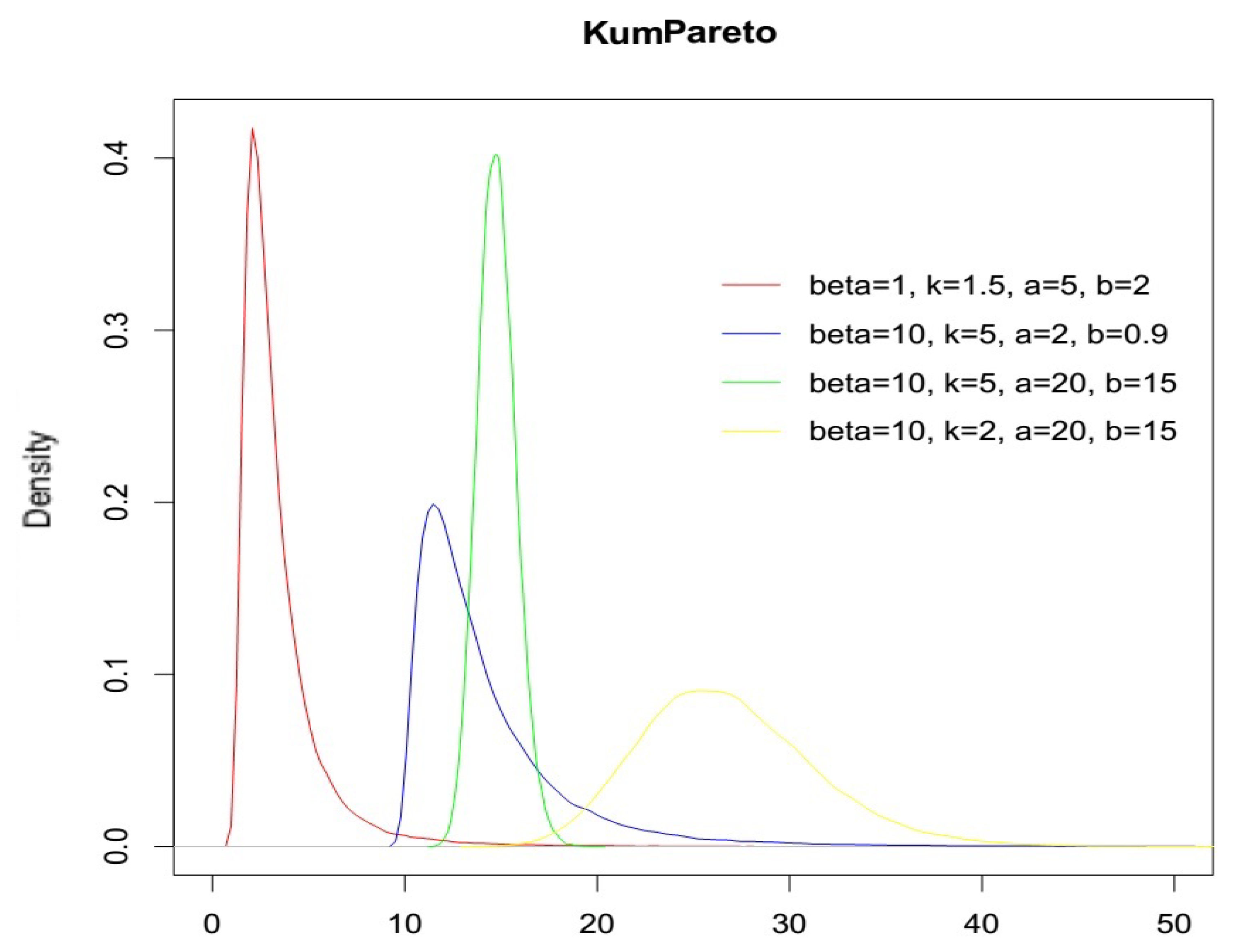
. In the following
Figure 2 we report the KumPareto density function varying the parameters:
4. Numerical Example of Composite Models
In this section we present numerical results on the fitting of Danish fire insurance data by composite models with constant and random thresholds between attritional and large claims. As already mentioned, for the composite models with a constant threshold, we used the methodology described in
Teodorescu and Vernic (
2009,
2013), obtaining
u = 1,022,125€.
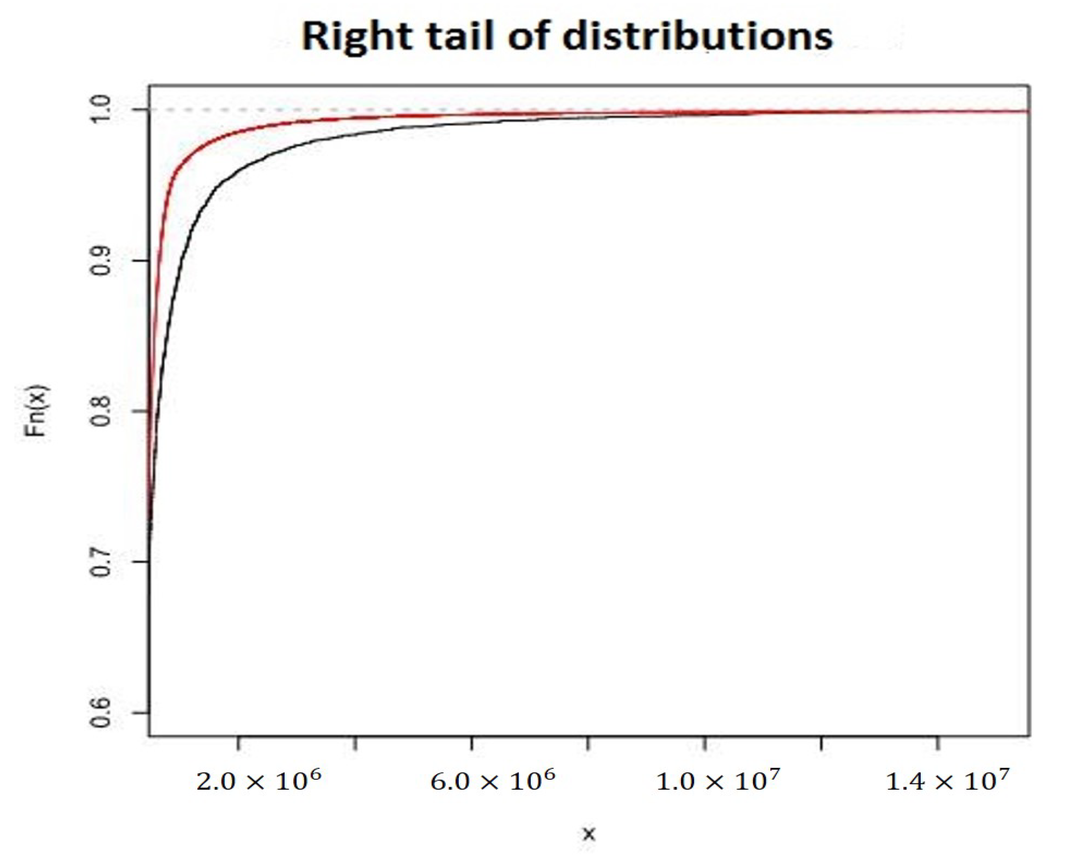
We start with a composite Lognormal–KumPareto model, choosing
and
. From the following
Table 4 we can compare some theoretical and empirical quantiles:
Only the fiftieth percentile of the theoretical distribution function was very close to the same empirical quantile: From this percentile onwards the differences increased. In the following
Figure 3 we show only right tails of the distribution functions (empirical and theoretical):
The red line is always above the dark line. This means Kumaraswamy-generalized families of distributions are very versatile in analyzing different types of data, but in this case the Lognormal–KumPareto model underestimated the right tail.
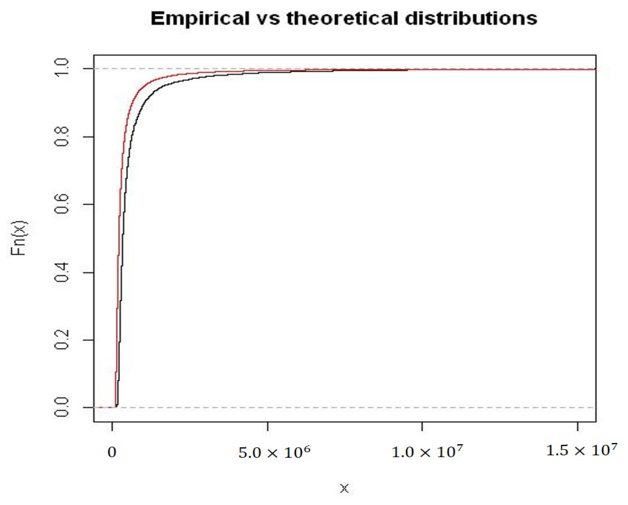
Therefore, we consider the composite model
and
as suggested in
Nadarajah and Bakar (
2014). The parameters are estimated using the CompLognonormal R package as shown in
Nadarajah and Bakar (
2014). From the following
Table 5 we can compare some theoretical quantiles with empirical ones:
This model seemed to be more feasible in catching the right tail of the empirical distribution with respect to the previous Lognormal–KumPareto, as we can see from the
Figure 4 below:
Similar to the Lognormal–KumPareto model, the Lognormal–Burr distribution line is always above the empirical distribution line but not always at the same distance.
We go forward modeling a Lognormal–Generalized Pareto Distribution (GPD), that is we choose
and
and then we generate pseudo-random numbers from quantile function (
10). In
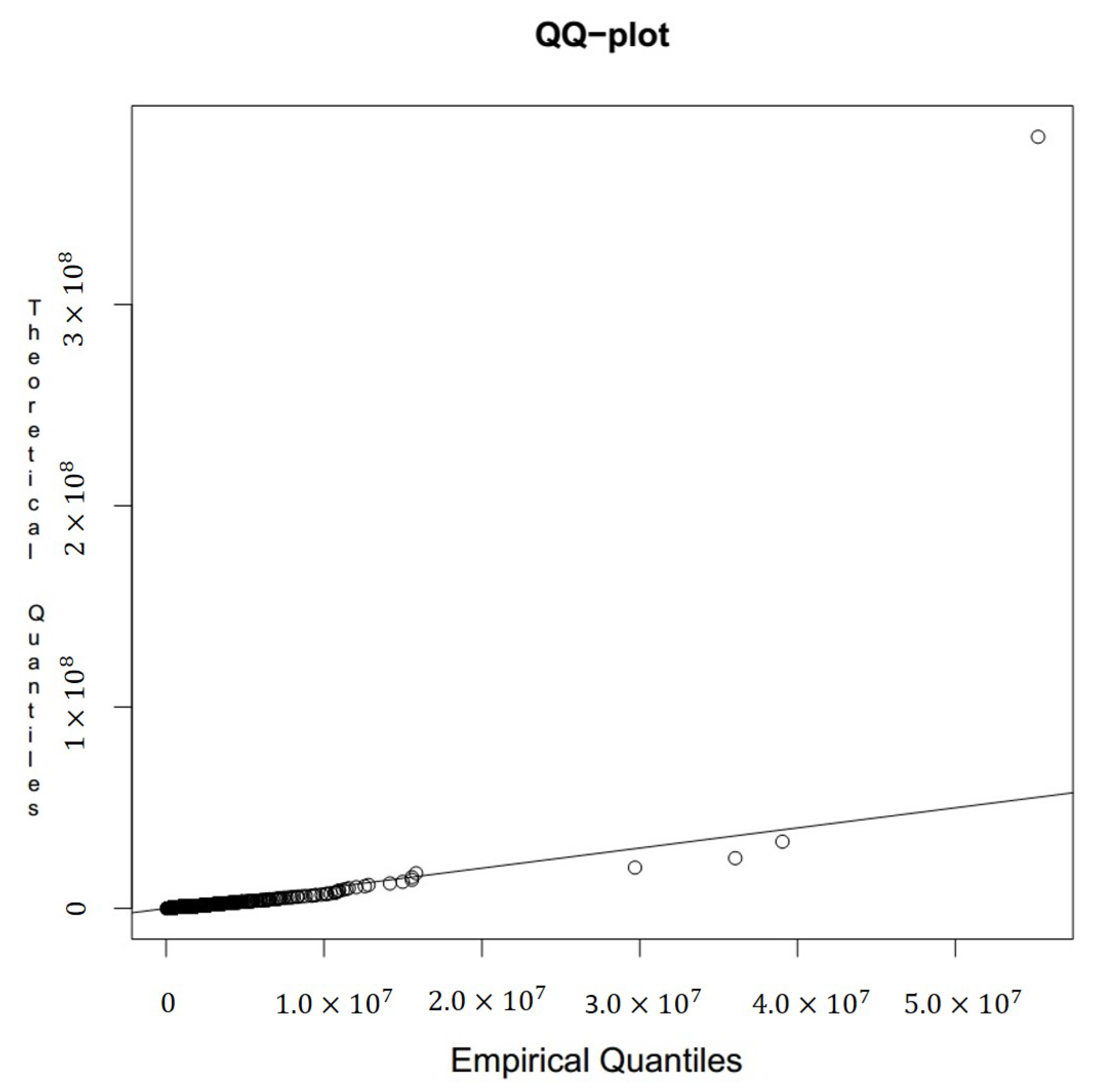
Table 6 and
Figure 5 we report the estimates of parameters, 99% confidence intervals and the QQ plot (
and
are the Lognormal parameters, while
and
are GPD parameters):
We observe that this composite model adapted well to the empirical distribution; in fact, except for a few points, theoretical quantiles are close to corresponding empirical quantiles. In the
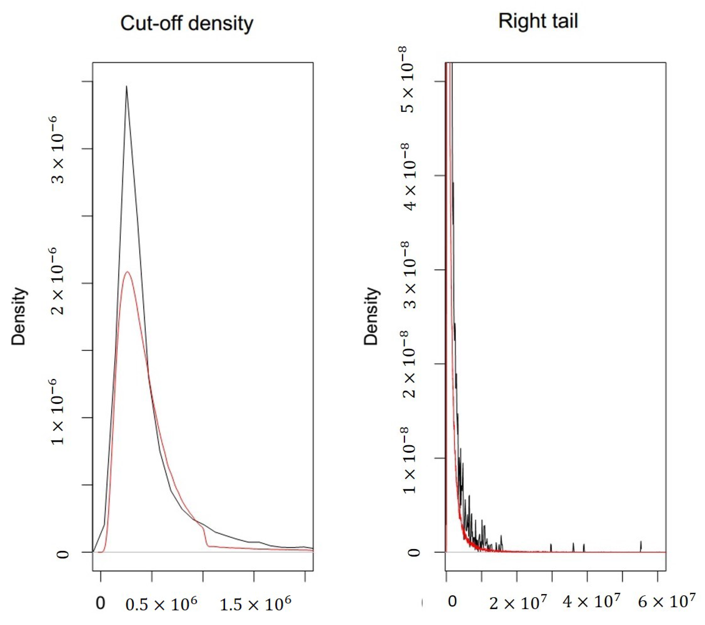
Figure 6 and
Figure 7 we compare the theoretical cut-off density function with the corresponding empirical one and the theoretical right tail with the empirical one.
The model exhibited a non-negligible right tail (kurtosis index is 115,656.2), which can be evaluated comparing the observed distribution function with the theoretical one.
The corresponding Kolmogorov–Smirnov test returned a p-value equal to 0.8590423, using 50,000 bootstrap samples.
Finally, in
Table 7 we report the best estimate and 99% confidence intervals of the composite model Lognormal–GPD with a Gamma random threshold
u (see
Pigeon and Denuit 2011).
The threshold
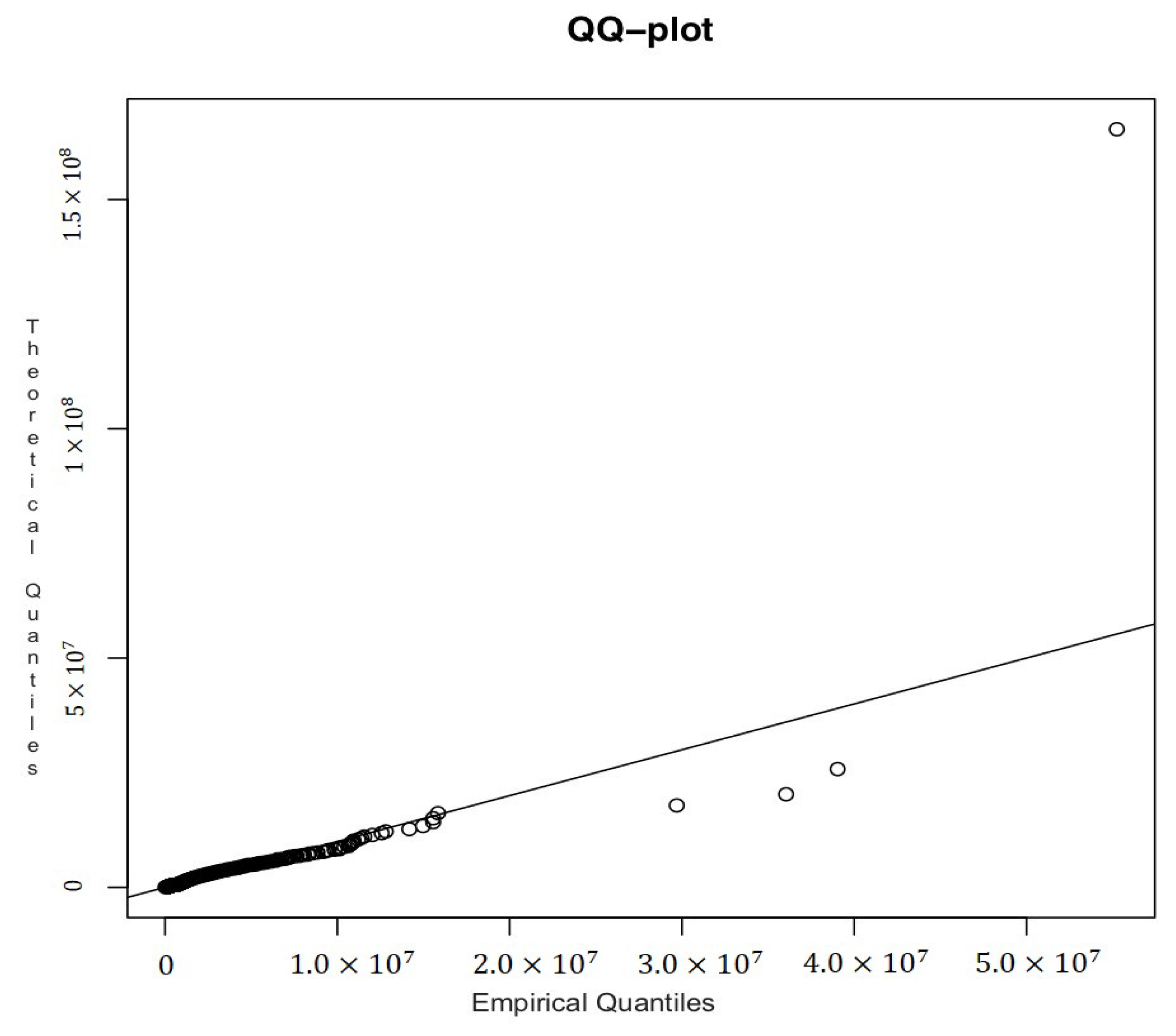
u is a parameter whose value depends on Gamma parameters. In the following
Table 8 and
Figure 8 we report the theoretical and empirical quantiles and the QQ plot.
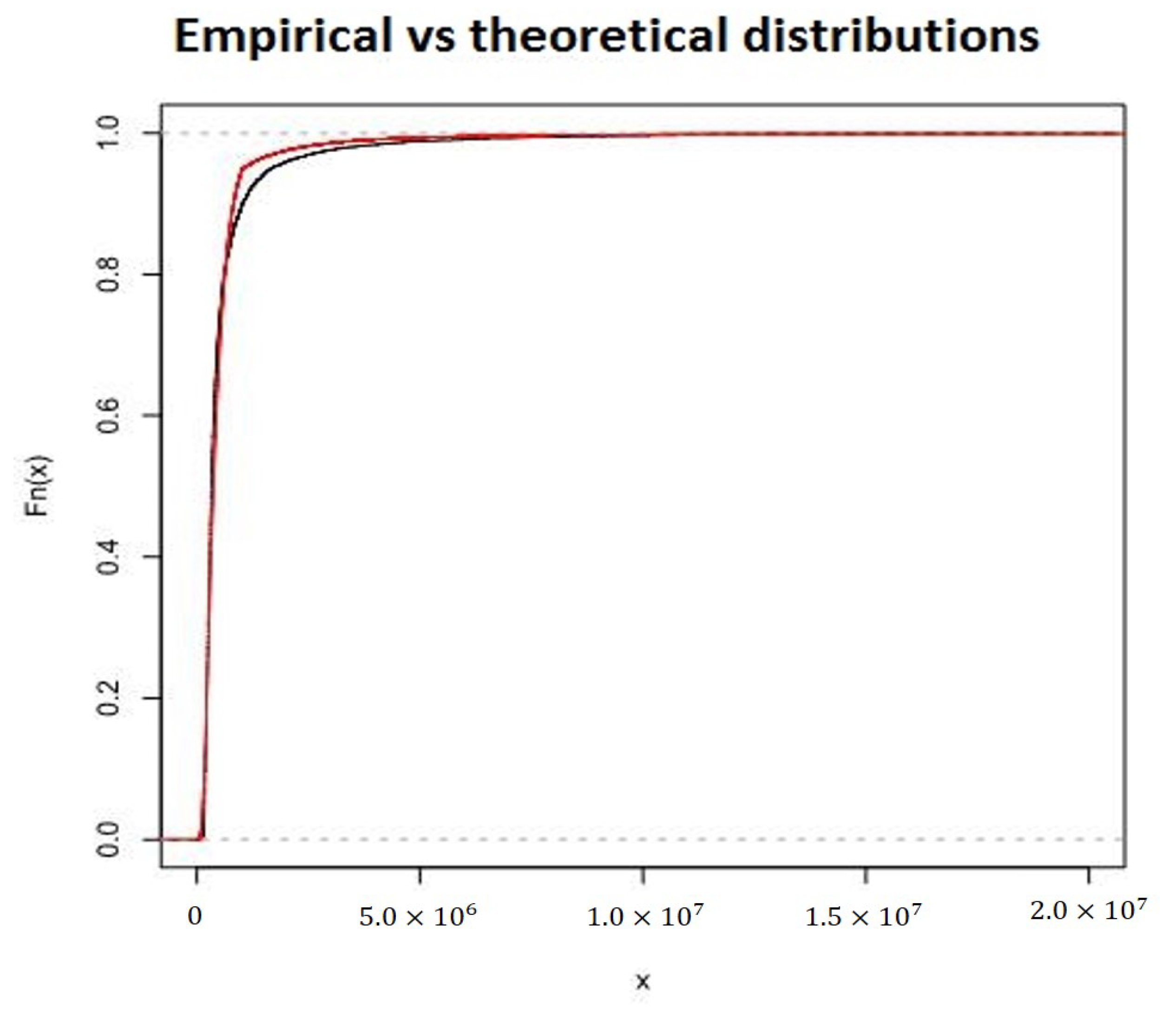
We can see from the
Figure 9 that Lognormal–GPD–Gamma model can be considered a good fitting model.
The Kolmogorov–Smirnov adaptive test returned p-value equal to 0.1971361; therefore, we cannot reject the null hypothesis under which the investigated model is a feasible model for our data.
Finally, Lognormal–KumPareto, Lognormal–Burr, Lognormal–GPD with fixed threshold and Lognormal–GPD with a Gamma random threshold can be compared using the AIC and BIC values,
Table 9.
The previous analysis suggests that the Lognormal–GPD–Gamma gives the best fit.
5. Introducing Dependence Structure: Copula Functions and Fast Fourier Transform
In the previous section we restricted our analysis to the case of independence between attritional and large claims. We now try to extend this work to a dependence structure. Firstly, we defined a composite model using a copula function to evaluate the possible dependence. As marginal distributions, we referenced to a Lognormal distribution for attritional claims and a GPD for large ones. The empirical correlation matrix
R
and Kendall’s Tau and Spearman’s Rho measures of association
suggest a weak but positive correlation between normal and large claims.
For this reason, the individuation of an appropriate copula function will not be easy, but we present an illustrative example based on a Gumbel Copula. We underline that an empirical dependence structure is inducted by distinction between attritional and large losses. In fact, there is no unique event that causes small and large losses simultaneously, but when an insured event occurs, only an attritional or large loss is produced. For this reason, the results showed in the following should be considered as an exercise that highlights the important effects of dependence on the aggregate loss distribution.
Table 10 reports the different methods to estimate the parameter
:
We remind that Gumbel’s parameter
assumes values in
, and for
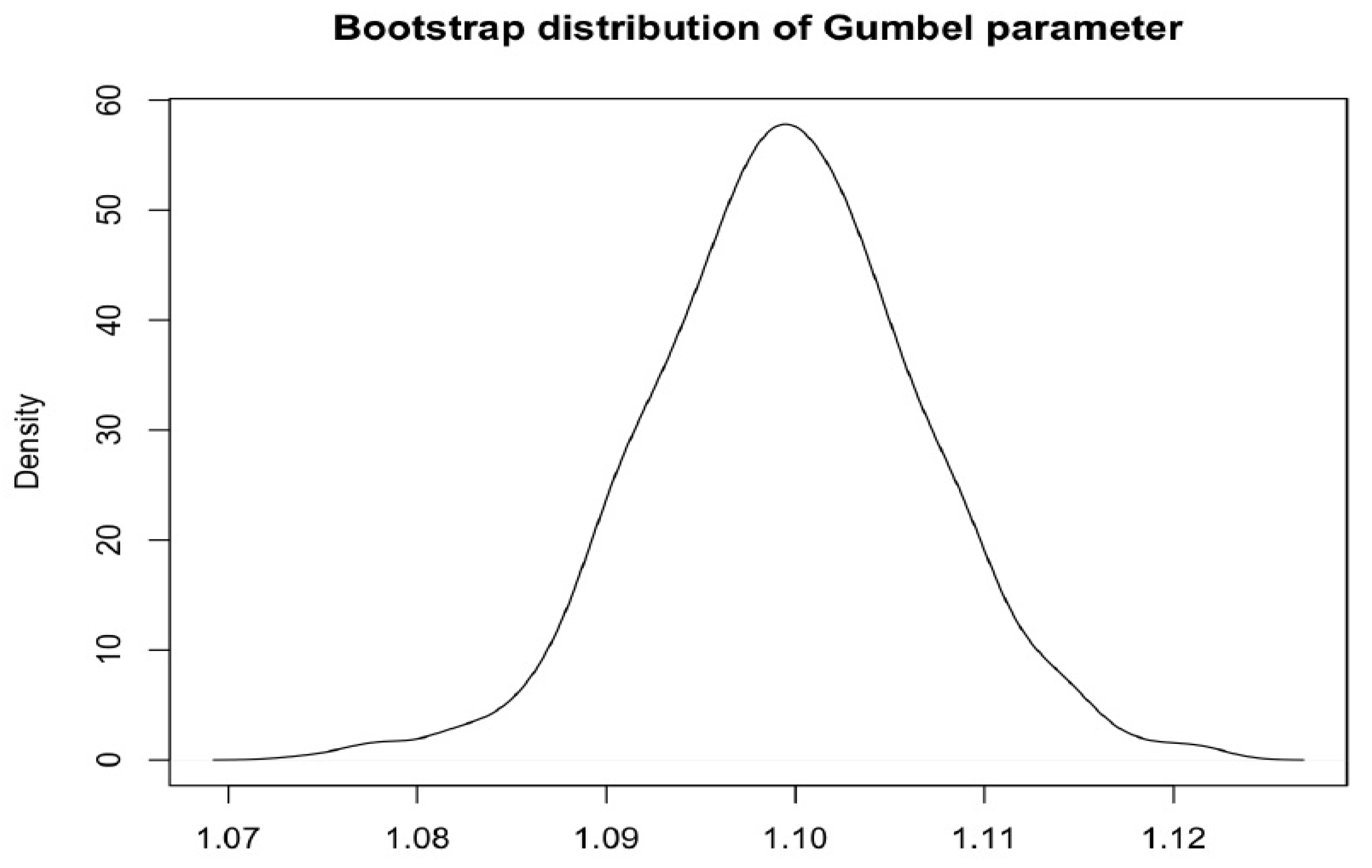
we have independence between marginal distributions. We observe that estimates were significantly different from 1, and so our Gumbel Copula did not correspond to the Independent Copula. We can say that because we verified using bootstrap procedures, the
parameter has a Normal distribution. In fact, the Shapiro–Wilk test gave a
p-value equal to 0.08551; thus, with a fixed significance level of 5%, it is not possible reject the null hypothesis. In addition, the 99% confidence interval obtained with Maximum pseudo-likelihood method was (1.090662; 1.131003), which does not include the value 1; the same confidence interval obtained with the Bootstrap procedure was (1.090662; 1.131003). In the following
Figure 10 we report the distribution of the Gumbel parameter obtained by the bootstrap procedure.
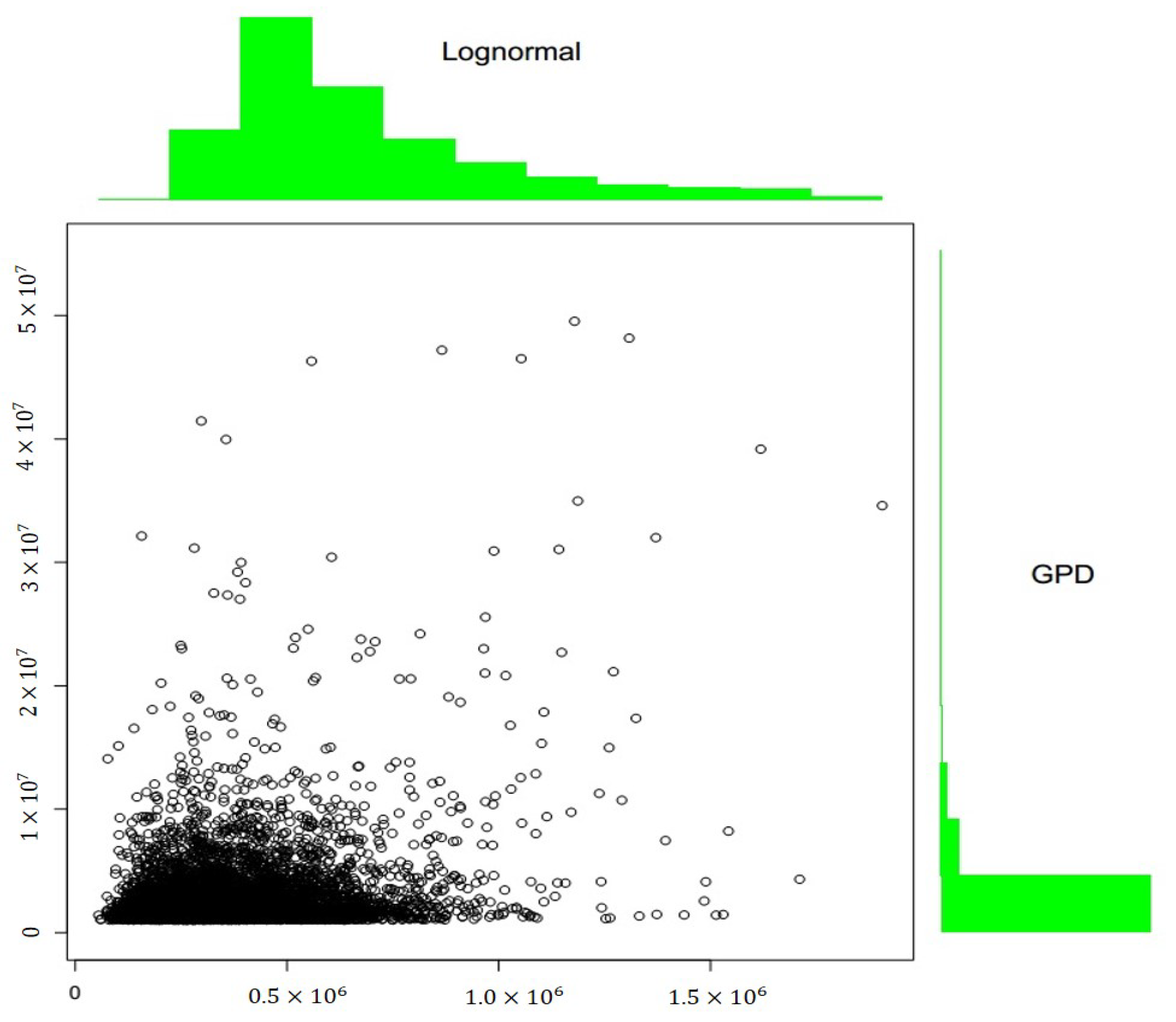
We report two useful graphics (
Figure 11 and
Figure 12), obtained by simulation of the estimated Gumbel.
The density function (
Figure 12) assumed greater values in correspondence of great values both for Lognormal and GPD marginal; in other words, using the Gumbel Copula, the probability that attritional claims produced losses near to the threshold u, and that large claims produced extreme losses, was greater than the probability of any other joined event.
We report also the result of the parametric bootstrap goodness-of-fit test performed on the estimated Gumbel Copula.
| Statistic | | p-Value |
| 2.9381 | 1.1108 | 0.00495 |
We can consider the estimated Gumbel a good approximation of dependence between data. In our numerical examples, we referred to the Gumbel Copula function despite having estimated and analyzed other copulas for which there was no significant difference for the aims of this paper. While the empirical dependence is not excessive, we will see how the introduction in the estimation model of a factor that takes it into account, such as a Copula function, will produce a non-negligible impact on the estimate of the VaR.
An Alternative to the Copula Function: The Fast Fourier Transform
Considering the fact that it is not easy to define an appropriate copula for this dataset, we next modeled the aggregate loss distribution directly with the Fast Fourier Transform (FFT) using empirical data. That approach allowed us to avoid the dependence assumption between attritional and large claims (necessary instead with the copula approach).
To build an aggregate loss distribution by FFT, it is first necessary to discretize the severity distribution Z (see
Klugman et al. 2010) and obtain the vector
, of which element
is the probability that a single claim produces a loss equal to
, where
c is a fixed constant such that, given
n length of vector
z, the loss
has a negligible probability. We considered also frequency claim distribution
through Probability-Generating function (PGF) defined as
In particular, let
and
be the FFT and its inverse, respectively. We obtain the discretized probability distribution for the aggregate loss X as
Both
and
are n-dimensional vectors whose generic elements are, respectively,
where
.
From a theoretical point of view, this is a discretized version of Fourier Transform (DFT):
The characteristic function created an association between a probability density function and continuous complex one, while the DFT made an association between an n-dimensional vector and an n-dimensional complex vector. The former one-to-one association can be done through the FFT algorithm.
For a two-dimensional case, matrix M
Z is a necessary input; this matrix contains joined probabilities of attritional and large claims such that it is possible to obtain corresponding marginal distributions by adding long rows and columns respectively. For example, let
be that matrix. The vector (0.5, 0.45, 0.05), obtained by adding long three rows, contains the marginal distribution of attritional claims, while the vector (0.7, 0.3, 0), obtained by adding long three columns, contains the marginal distribution of large claims. The single element of the matrix, instead, is the joined probability. The aggregate loss distribution will be a matrix
given by
We decided to discretize the observed distribution function, without reference to a specific theoretical distribution, using the discretize R function available in the actuar package (see
Klugman et al. 2010). This discretization allows us to build the matrix
to which we applied the two-dimensional FFT version. In this way, we obtained a new matrix
that acted as input for the random
probability generating function.
As reported in
Section 2, in our dataset, 50% of frequencies were included between 238 and 381 claims, and there was a slightly negative asymmetry. In addition, the variance was greater than the mean value (299). Thus, it is possible to suppose a Negative Binomial distribution for frequency claims. The corresponding probability generating function is defined by
We estimated its parameters that resulted and . Then, we obtained the matrix . As the last stage we applied the IFFT whose output is matrix . Adding long counter-diagonals of we can individuate the discretized probability distribution of aggregate loss claims, having maintained the distinction between normal and large claims and, above all, preserving the dependence structure.
6. Final Results and Discussion
As shown previously, from the perspective of strict adaptation to empirical data, we can say that the best model to fit the Danish fire data is the Lognormal–GPD–Gamma one, which presented a coefficient of variation equal to 10, 2%, lesser than Standard Formula volatility. In fact, considering the premium risk and Fire segment only, the volatility of the Standard Formula was equal to 24% (3 times
, where
; see
Tripodi 2018). As written in the introduction of the present work, this result mainly was due to the fact that the DA multiplier did not take into account the skewness of the aggregate claim distribution, and it potentially overestimated the SCR for large insurers.
For illustrative purposes only, we estimated the and the volatility of aggregate loss using the previous models, taking into account a dependence structure as well. According to the collective approach of risk theory, aggregate loss is the sum of a random number of random variables, and so it requires convolution or simulation methods. We remember that among the considered methodologies, only FFT directly returned the aggregate loss. Relating to FFT, as we mentioned above, an empirical dependence structure was inducted by discriminating between attritional and large losses, so we referred to empirical discretized severities in a bivariate mode. This is a limitation of our work that could be exceeded considering a bivariate frequency and two univariate severities, inducting such dependence by the frequency component, as it happens in practice (i.e., dependency between severities is not typical for this line of business); however, this approach would not have allowed us to apply the FFT methodology.
Considering the statistics of frequency in the Danish fire insurance data, we can assume claim frequency k distributed as a Negative Binomial, as done previously with the FFT procedure. A single simulation of aggregate loss can be achieved by adding the losses of k single claims, and by repeating the procedure n times, we obtained the aggregate loss distribution.
Contrary to the copula approach, we point out that it would be possible to obviate the need to simulate by applying FFT to generate aggregates from the fit severities.
In
Table 11, we report the VaRs obtained using composite models Lognormal–GPD–Gamma, Gumbel Copula and FFT, and the corresponding coefficients of variation that give us indications of the applied models’ volatilities:
If we consider the independence assumption, the aggregate loss distribution will return a VaR significantly smaller (over −200%) than that calculated using the dependence hypothesis. The assumption of independence, or not, would therefore produce obvious repercussions on the definition of the risk profile and, consequently, on the calculation of the capital requirement. As seen above, for the case analyzed, the Gumbel Copula took into account the positive dependence, even if of discrete magnitude, between the tails of the marginal distributions of the severities. That is, an attritional loss close to the discriminatory threshold is, with good probability, accompanied by an extreme loss. This can only induce a decisive increase in the VaR of the aggregate distribution, as can be seen from
Table 11. In the same way as Fast Fourier Transform, taking into account not only the (empirical) dependence between claims but also the randomness of frequency claims also induces a further increase in the risk estimate.
Therefore, it is fundamental to take into account the possible dependence between claims, regarding its shape and intensity, because the VaR could increase drastically with respect to the independence case, leading to an insolvent position of the insurer.This analysis highlights the inadequacy of using CV when the actual objective is to estimate VaR.
However, all previous approaches have advantages and disadvantages. With the composite models we can robustly fit each of the two underlying distributions of attritional and large claims, without a clear identification of the dependency structure. With the Copula we can model dependency, but it is not easy to determine what is the right copula to use, and this is the typical issue companies have to face for capital modeling purposes using a copula approach. FFT allows one to not simulate the claim process and to not estimate a threshold, working directly on empirical data, but includes some implicit bias due to the discretization methods; for example, since the FFT works with truncated distributions, it can generate aliasing errors. We point again to
Robe-Voinea and Vernic (
2016) and
Robe-Voinea and Vernic (
2017) for a detailed discussion and the possible solutions insurers have to consider when implementing PIM.
Finally, compared to the present literature, we remark that this paper innovates the fitting of the Danish fire insurance data, using a composite model with a random threshold. Secondly, our empirical model could have managerial implications, supporting insurance companies in understanding that the Standard Formula could lead to a volatility (and the SCR) of the premium risk that is very different from the real risk profile. It is worth mentioning
CEIOPS (
2009), in that “Premium risk also arises because of uncertainties prior to issue of policies during the time horizon. These uncertainties include the premium rates that will be charged, the precise terms and conditions of the policies and the precise mix and volume of business to be written. Various studies (e.g.,
Mildenhall (
2017)
Figure 10) have shown that pricing risk results in a substantial increase in loss-volatility, especially for commercial lines”. Therefore, one would expect that the SCR premium charge would look high compared to a test that only considers loss (frequency and severity) uncertainty. In next developments of this research we will try to take into account these features in order to have a full picture of this comparison.


