A Two-Population Extension of the Exponential Smoothing State Space Model with a Smoothing Penalisation Scheme

Abstract

The joint modelling of mortality rates for multiple populations has gained increasing popularity in areas such as government planning and insurance pricing. Sub-groups of a population often preserve similar mortality features with short-term deviations from the common trend. Recent studies indicate that the exponential smoothing state space (ETS) model can produce outstanding prediction performance, while it fails to guarantee the consistency across neighbouring ages. Apart from that, single-population models such as the famous Lee-Carter (LC) may produce divergent forecasts between different populations in the long run and thus lack the property of the so-called coherence. This study extends the original ETS model to a two-population version (2-ETS) and imposes a smoothing penalisation scheme to reduce inconsistency of forecasts across adjacent ages. The exponential smoothing parameters in the 2-ETS model are fitted by a Fourier functional form to reduce dimensionality and thus improve estimation efficiency. We evaluate the performance of the proposed model via an empirical study using Australian female and male population data. Our results demonstrate the superiority of the 2-ETS model over the LC and ETS as well as two multi-population methods - the augmented common factor model (LL) and coherent functional data model (CFDM) regarding forecast accuracy and coherence.

1. Introduction

Continual improvements in human life expectancies over the past few decades have brought a serious challenge to the prediction of future mortality scenarios. Mortality forecasts are crucial not only in demography but also in many other relevant areas. Accurate forecasts are therefore essential to government planning, designing of pension schemes and annuity products and the reserving for insurance companies.

Actuaries and researchers have developed various models to describe and predict features of mortality reductions. One of the most famous models is the Lee-Carter (LC) (Lee and Carter 1992) model belonging to the extrapolative family whose members produce predictions by assuming the continuity of past patterns. Many developments and extensions have been proposed to the single-population LC model. For example, Renshaw and Haberman (2006) incorporate an additional cohort factor to capture the pattern related to the year of birth. Li and Lee (2005) develop a multi-population version of the LC which is referred to as the augmented common factor model (LL).

Although the LC model receives criticisms for its insufficient allowance for potential volatility in mortality forecasts (see, for example, Wong et al. 2020), it has been regarded as a benchmark in various studies. For instance, Feng and Shi (2018) adopt the exponential smoothing state space (ETS) model1 to predict mortality rates and compare its performance with those under the LC, functional data model (FDM) as well as some univariate time series processes. Thereinto, the ETS model turns out to be the best-performing choice based on Australian population data. According to Makridakis and Hibon (2000), the ETS model also presents outstanding results in the M3-competition. However, fitting a single-population ETS model without constraints/penalties may be incapable of ensuring the coherence, which is important in long-run forecast of mortality rates (Li and Lu 2017; Li 2013; Li and Lee 2005). As indicated by our empirical studies, the mortality forecasts of the single-population ETS model suffer from the limitation that rates of adjacent ages may be inconsistent with one another in the long run. In other words, it is possible to generate significant fluctuations for certain age groups, which can cause problems when using such forecasts to price annuities and mortality-linked securities. Furthermore, in the case of modelling multiple populations, single-population models such as the LC and ETS cannot ensure consistency between populations, and hence lose the critical property of coherence. It would be more desirable to perform a joint modelling of two or more related groups and integrate their relationships into mortality forecasts. For example, it is biologically unreasonable to predict that future mortality rates of males and females in the same country will diverge over time.

Our study overcomes the above issues of the original ETS model by imposing a smoothing penalisation scheme as described in Li and Lu (2017) and extending it to a two-population ETS model (2-ETS). Under the proposed model, the rates of mortality changes for sub-populations under investigation are associated with each other, enabling coherent forecasts for the whole group. More specifically, the smoothness across adjacent ages is guaranteed by setting parameters which minimise the sum of squared differences of mortality changes between neighbouring ages. However, the 2-ETS model involves hundreds of parameters and is difficult to estimate because no close-form solutions are available from its iterative identification procedure. To improve the fitting efficiency, we employ the Fourier dimensionality reduction technique. In particular, a Fourier functional form is fitted to each of the exponential smoothing parameters in the 2-ETS model, so that the original group of unknown parameters is reduced to a dozen of Fourier factors.

To examine the performance of the 2-ETS model, we compare its prediction results with those under the benchmark LC model and the original ETS model. Besides these two single-population candidates, the multi-population extensions of LC and FDM – the LL and coherent functional data model (CFDM) developed by Hyndman et al. (2012) are added to the comparison list. Using Australian female and male population data over 1950–2016 and ages 0–100, we demonstrate the superiority of the proposed 2-ETS model over the other candidates under various scenarios. Based on simulated replicates with multi-Gaussian distributed residuals, the prediction intervals (PIs) also accurately capture the true data, when mortality rates averaged over all ages are used.

In summary, this paper develops a two-population ETS model with a smoothing penalisation scheme and compares its performance with other popular alternatives. The proposed model ensures the desirable coherence property and can improve the superior forecasting results of the original single-population ETS model. The remaining of the article is structured as follows. Section 2 reviews specifications of the LC, ETS, LL and CFDM models. Section 3 specifies the 2-ETS model and describes the fitting procedure. An empirical study comparing the five mortality models is reported in Section 4. Finally, Section 5 gives concluding remarks and possible directions for future research.

2. Model Description

2.1. The Lee-Carter Model

The Lee-Carter (LC) model is proposed by Lee and Carter (1992). It expresses the log central mortality rate at age x in year t as

$$ln{m}_{x,t}=a_x+b_x{k}_t+{\epsilon }_{x,t},$$

(1)

where $a_x$ is the average mortality level at each age, $k_t$ is the mortality index at time t, $b_x$ represents the age-specific sensitivity of $ln{m}_{x,t}$ to changes in $k_t$, and ${\epsilon }_{x,t}$ is the error term with null mean. Since the right-hand side parameters are not observable, they are estimated by singular value decomposition (SVD) instead of the usual ordinary least square approach in the original paper.2 To avoid the identification problem, two constraints ${\sum }_t{k}_t=0$ and ${\sum }_x{b}_x=1$ are imposed. As implied by the first constraint, the age effect $a_x$ is set to the mean of log central death rates across years. Given the estimated $a_x$ and $b_x$, $k_t$ is adjusted to match the fitted total number of deaths to the observed values in each year t. The reconciliation rebalances the equal contribution by mortality at all ages by assigning greater weights to ages at which death counts are larger.

Under the LC model, the two age-specific parameters are assumed to remain unchanged over time, and the mortality index is often modelled by a random walk with drift as follows:

$$k_t=k_{t-1}+d+e_t,$$

(2)

where the drift term d measures the average annual change in $k_t$, and $e_t\sim N(0,{\sigma }_e^2)$. As suggested by Giacometti et al. (2012), the expected h-step-ahead forecast of the mortality index and the log central death rate can be calculated as:

$$\begin{array}{cc}\hfill {\widehat{k}}_{T+h}=k_T+& hd=k_T+h\frac{k_T-k_1}{T-1}\hfill \\ \hfill ln{\widehat{m}}_{x,T+h}& =a_x+b_x{\widehat{k}}_{T+h}\hfill \end{array},$$

(3)

where T is the end of the fitting period.

2.2. Exponential Smoothing State Space (ETS) Model

One popular category of forecasting models is called exponential smoothing model under which forecasts are produced as a weighted sum of past values. Members of this family assign exponentially decaying weights to observations further into the past rather than using a simple average (Hyndman et al. 2008).

Pegels (1969) proposes a way to classify ETS models according to the combination of various types of error, trend and seasonal components involved in the model. This list has been extended to thirty distinct ETS models by employing additive/multiplicative error/trend/seasonality components. Thereinto, a ’damped’ type can be added to characteristics of the trend component, implying a flattened trend of predictions (Gardner and Mckenzie 1985). For instance, Gardner (1985) introduces an ETS model with an additive damped trend, which is then modified by Taylor (2003) to a multiplicative one. Besides, it has been shown that exponential smoothing models can be expressed as innovations state space models (Hyndman et al. 2002, 2005). Detailed model specifications can be found in Section 2 of Hyndman and Khandakar (2008).

Nevertheless, ETS models with seasonal components are not applicable to our study because seasonality is not present in mortality forecasting. In addition, Feng and Shi (2018) suggest that only two ETS models (with additive (damped) trend and additive error terms) are possibly suitable for modelling mortality rates. We do not consider the ETS model with damped trend in this paper.3 Expression of the only appropriate ETS specification (also known as the Holt-Winters model) is described as follows:

$$\begin{array}{cc}\hfill ln{m}_{x,t}& =l_{x,t-1}+b_{x,t-1}+{\epsilon }_{x,t}\hfill \\ \hfill l_{x,t}& =l_{x,t-1}+b_{x,t-1}+{\alpha }_x{\epsilon }_{x,t}\hfill \\ \hfill b_{x,t}& =(1-{\beta }_x)b_{x,t-1}+{\beta }_x(l_{x,t}-l_{x,t-1})\hfill \end{array},$$

(4)

where $l_{x,t}$ and $b_{x,t}$ represent the level and growth of $ln{m}_{x,t}$, respectively. Their corresponding exponential smoothing parameters ${\alpha }_x$ and ${\beta }_x$ can be computed by minimising ${\sum }_{x,t}{\epsilon }_{x,t}^2$, but no close-form solutions are available from the iterative estimation procedure. The h-step-ahead forecast of the log mortality rate is

$$ln{\widehat{m}}_{x,T+h}=l_{x,T}+h{b}_{x,T},$$

(5)

where T is the end of the fitting period.

When modelling mortality of multiple populations, the above two single-population models may fail to ensure coherence. For example, separate forecasts for female and male mortality generated from single-population models may diverge over time. A more formal discussion of the coherence can be found in Section 3.1. To ensure this desirable feature, we also consider two popular multi-population models.

2.3. The Augmented Common Factor, or Lee-Li (LL) Model

Li and Lee (2005) extend the Lee-Carter model by introducing an additional common factor which controls the relationships between populations. Specifically, the log central death rate is modelled as:

$$ln{m}_{x,t,i}=a_{x,i}+B_x{K}_t+b_{x,i}{k}_{t,i}+{\epsilon }_{x,t,i},$$

(6)

where $a_{x,i}$ represents the average of the age-specific mortality level for the ith population, $B_x$ and $K_t$ represent the age effect and period effect of the common factor, $k_{t,i}$ is the time component of the ith population with age response $b_{x,i}$, and ${\epsilon }_{x,t,i}$ is the population-specific error term.

The common factor $B_x{K}_t$ describes the mortality trend of all populations. In the original work of Li and Lee (2005), it is estimated from applying the LC method to the total population, subject to constraints ${\sum }_t{K}_t=0$ and ${\sum }_x{B}_x=1$. Then $a_{x,i}$ is obtained by minimising the modelling error of each subpopulation ${\sum }_t{(ln{m}_{x,t,i}-a_{x,i}-B_x{K}_t)}^2$ at age x. Implied by the constraint on $K_t$, $a_{x,i}$ is taken as the average of $ln{m}_{x,t,i}$ over t. The population-specific factor $b_{x,i}{k}_{t,i}$ can be estimated by applying SVD to the residual matrix $(ln{m}_{x,t,i}-a_{x,i}-B_x{K}_t)$.

Similar to the case under LC, the common mortality index $K_t$ can be modelled as a random walk with drift process. On the other hand, the group-specific time component $k_{t,i}$ is fitted by a stationary autoregressive process to ensure coherent forecasts in the long term. Specifically,

$$\begin{array}{cc}\hfill K_t& =K_{t-1}+d+e_t\hfill \\ \hfill k_{t,i}& ={\alpha }_{0,i}+{\alpha }_{1,i}{k}_{t-1,i}+e_{t,i}\hfill \end{array},$$

(7)

where ${\alpha }_{0,i}$ and ${\alpha }_{1,i}$ are the autoregressive parameters and $e_{t,i}$ is the Gaussian error term with null mean. The stationarity guarantees that deviations of each population from the common trend will not continue in the long run. Given the data observed in the last year T, the h-step-ahead forecast of the log central death rate is given as follows:

$$ln{\widehat{m}}_{x,T+h,i}=a_{x,i}+B_x{\widehat{K}}_{T+h}+b_{x,i}{\widehat{k}}_{T+h,i}.$$

(8)

2.4. The Coherent Functional Data Model (CFDM)

Hyndman et al. (2012) propose a mortality model with coherent forecasting, which is developed from the single-population functional data model (Hyndman and Shahid Ullah 2007). Instead of working on mortality rates directly, the coherent functional data model (CFDM) predicts the product and ratio functions of mortality rates for different groups. Considering the case with I populations, the product and ratio functions are given as

$$\begin{array}{cc}\hfill p_{x,t}& ={\left(\prod _{i=1}^I{m}_{x,t,i}\right)}^{1/I}\hfill \\ \hfill r_{x,t,i}& =m_{x,t,i}/p_{x,t}\hfill \end{array},$$

(9)

where $m_{x,t,i}$ is the central death rate of population i ($i=1,2,\cdots ,I$). Therefore, the CFDM is also referred to as the product-ratio model, which can be expressed as:

$$\begin{array}{cc}\hfill ln{p}_{x,t}& ={\mu }_{x,p}+\sum _{j=1}^J{\varphi }_{t,j}{\beta }_{x,j}+{\epsilon }_{x,t}\hfill \\ \hfill ln{r}_{x,t,i}& ={\mu }_{x,r,i}+\sum _{g=1}^G{\psi }_{t,g,i}{\gamma }_{x,g,i}+{\epsilon }_{x,t,i}\hfill \end{array},$$

(10)

where ${\mu }_{x,p}$ and ${\mu }_{x,r,i}$ are the average of $ln{p}_{x,t}$ and $ln{r}_{x,t,i}$ across years, ${\epsilon }_{x,t}$ and ${\epsilon }_{x,t,i}$ are serially uncorrelated error terms with zero mean, and the principal factors ${\beta }_{x,j}$, ${\gamma }_{x,g,i}$ and their corresponding component scores ${\varphi }_{t,j}$, ${\psi }_{t,g,i}$ are obtained using the weighted principal components analysis (Hyndman and Shang 2009). This fitting technique assigns higher weights to more recent data, which avoids the problem of potential time-varying age components (Lee and Miller 2001).

Both the number of principal factors for product and ratio functions are set to be 6 ($J=G=6$) which is the optimal choice balancing forecast accuracy and parameter parsimony (Hyndman et al. 2012). Those time-varying components of the product function govern the main trend of future mortality rates and are forecasted by non-stationary processes. Nonetheless, stationarity is required in modelling the period effects for the ratio function to ensure the non-divergence of mortality projections. The h-step-ahead forecast of log central death rates for each subpopulation can be calculated as

$$\begin{array}{cc}\hfill ln{\widehat{m}}_{x,T+h,i}& =ln\left({\widehat{p}}_{x,T+h}{\widehat{r}}_{x,T+h,i}\right)\hfill \\ \hfill & ={\mu }_{x,i}+\sum _{j=1}^J{\widehat{\varphi }}_{T+h,j}{\beta }_{x,j}+\sum _{g=1}^G{\widehat{\psi }}_{T+h,g,i}{\gamma }_{x,g,i}\hfill \end{array},$$

(11)

where T is the end of the fitting period, ${\mu }_{x,i}={\mu }_{x,p}+{\mu }_{x,r,i}$. While the prediction function is similar to that under the LL model, the CFDM model adopts six components for the common and population-specific factors rather than one.

3. The Two-Population ETS Model

Compared with a single-population model, the most outstanding merit of a multi-population model is the characteristic of coherence, which is defined as follows (Li and Lee 2005).

Definition 1.

Coherence means that the forecasts of $ln{m}_{x,t,i}$ and $ln{m}_{x,t,j}$ will not diverge for the mortality rate of the x-year-old of populations i and j, when $t\to \infty$.

Remark 1.

As argued in Li and Lee (2005) and Hyndman et al. (2012), respectively, the forecasts produced by LL and CFDM models are coherent.

Despite the outstanding forecasting performance of the ETS model presented in Feng and Shi (2018), the original ETS model is not feasible for multi-population modelling. In this section, we propose a two-population ETS model and demonstrate the existence of coherence in this framework.

3.1. Model Specification

In the original ETS model, it is worth noting from (5) that when h is large (indicating long-term forecasts), $ln{\widehat{m}}_{x,T+h}$ will be dominated by $b_{x,T+h}$. It is because $l_{x,T}$ is not changing with h and is therefore $o\left(h\right)$. Furthermore, the growth equation of (4) indicates that

$$b_{x,t}=(1-{\beta }_x)b_{x,t-1}+{\beta }_x(b_{x,t-1}+{\alpha }_x{\epsilon }_{x,t})=b_{x,t-1}+{\beta }_x{\alpha }_x{\epsilon }_{x,t}$$

which is a random walk without drift and thus an I(1) process. Therefore, within a multivariate (vectorized) framework, we will adopt the idea of co-integration. A related structure can be found in Li and Lu (2017), for which a two-population ETS (2-ETS) model can be specified as follows.

$$\begin{array}{cc}\hfill ln{m}_{x,t,i}& =l_{x,t-1,i}+b_{x,t-1,i}+{\epsilon }_{x,t,i}\hfill \\ \hfill l_{x,t,i}& =l_{x,t-1,i}+b_{x,t-1,i}+{\alpha }_{x,i}{\epsilon }_{x,t,i}\hfill \\ \hfill b_{x,t,i}& =(1-{\gamma }_{x,i})b_{x,t-1,i}+{\gamma }_{x,i}{b}_{x,t-1,-i}+{\beta }_{x,i}^{\ast }{\epsilon }_{x,t,i}\hfill \end{array}$$

(12)

where ${\beta }_{x,i}^{\ast }={\beta }_{x,i}{\alpha }_{x,i}$, $i=1,2$, and $-i=$1 (2) when $i=$2 (1).

The forecasting equations under the 2-ETS model are more complex than those produced in (4), which can be iteratively derived using

$$\begin{array}{cc}\hfill ln{\widehat{m}}_{x,T+h,1}=& l_{x,T,1}+\sum _{k=1}^h{b}_{x,T+k-1,1}\hfill \\ \hfill ln{\widehat{m}}_{x,T+h,2}=& l_{x,T,2}+\sum _{k=1}^h{b}_{x,T+k-1,2}\hfill \\ \hfill b_{x,T+k,1}=& (1-{\gamma }_{x,1})b_{x,T+k-1,1}+{\gamma }_{x,1}{b}_{x,T+k-1,2}\hfill \\ \hfill b_{x,T+k,2}=& (1-{\gamma }_{x,2})b_{x,T+k-1,2}+{\gamma }_{x,2}{b}_{x,T+k-1,1}\hfill \end{array}$$

(13)

Theorem 1.

Given that all ${\alpha }_{x,i}$, ${\beta }_{x,i}$ and ${\gamma }_{x,i}$ fall in (0,1) for all ages x and $i=1,2$, and ${\epsilon }_{x,t,i}$ follows a multi-Gaussian distribution with means 0 and covariance matrix ${\mathbf{\Sigma }}_{\mathit{i}}$ for each $i=1,2$, mortality rates forecasted by the 2-ETS model described in (12) are coherent.

Proof. 

We focus on the growth equations of the two populations. From (12), it can be shown that

$$\begin{array}{cc}\hfill b_{x,t,1}-b_{x,t,2}=& (1-{\gamma }_{x,1})b_{x,t-1,1}+{\gamma }_{x,1}{b}_{x,t-1,2}+{\beta }_{x,1}^{\ast }{\epsilon }_{x,t,1}\hfill \\ \hfill & -(1-{\gamma }_{x,2})b_{x,t-1,2}-{\gamma }_{x,2}{b}_{x,t-1,1}-{\beta }_{x,2}^{\ast }{\epsilon }_{x,t,2}\hfill \\ \hfill =& (1-{\gamma }_{x,1}-{\gamma }_{x,2})(b_{x,t-1,1}-b_{x,t-1,2})+{\beta }_{x,1}^{\ast }{\epsilon }_{x,t,1}-{\beta }_{x,2}^{\ast }{\epsilon }_{x,t,2}\hfill \end{array}$$

Thus, with the proposed constraints on ${\alpha }_{x,i}$, ${\beta }_{x,i}$ and ${\gamma }_{x,i}$, it can be seen that $(1-{\gamma }_{x,1}-{\gamma }_{x,2})\in (-1,1)$ and ${\beta }_{x,1}^{\ast },{\beta }_{x,2}^{\ast }\in (0,1)$. Thus, $b_{x,t,1}-b_{x,t,2}$ is I(0) and approaching 0 when $t\to \infty$. In other words, $b_{x,t,1}-b_{x,t,2}$ is a co-integration.

Consequently, using (13) we have that

$$\begin{array}{cc}\hfill ln{\widehat{m}}_{x,T+h,1}-ln{\widehat{m}}_{x,T+h,2}& =l_{x,T,1}-l_{x,T,2}+(b_{x,T,1}-b_{x,T,2})\sum _{k=0}^{h-1}{(1-{\gamma }_{x,1}-{\gamma }_{x,2})}^k\hfill \\ & \to l_{x,T,1}-l_{x,T,2}+(b_{x,T,1}-b_{x,T,2})/({\gamma }_{x,1}+{\gamma }_{x,2})\hfill \end{array}$$

when $t\to \infty$. Thus, the ratio ${\widehat{m}}_{x,T+h,1}/{\widehat{m}}_{x,T+h,2}$ will converge to a constant at each age and the death rates ${\widehat{m}}_{x,T+h,1}$ and ${\widehat{m}}_{x,T+h,2}$ will not diverge in the long run, which completes the proof. □

Remark 2.

The assumptions of the 2-ETS model are all standard and not strong. For example, ${\alpha }_{x,i}$, ${\beta }_{x,i}\in (0,1)$ is directly adopted from the single-population ETS model. ${\gamma }_{x,i}\in (0,1)$ is an analogous extension. The assumption of multi-Gaussian disturbances is popularly employed in the existing literature, such as Lee and Carter (1992), Hyndman et al. (2012) and Li and Lu (2017).

In addition to the coherence among populations, smoothness across neighboring age groups is also of interest in mortality forecasting. Thus, in terms of the estimation, we follow the smoothing penalisation scheme of Li and Lu (2017) by minimising4

$$\sum _{x=0}^{100}\sum _{t=1}^T\sum _{i=1}^2{\epsilon }_{x,t,i}^2+{\lambda }_1\sum _{x=0}^{99}{(b_{x+1,T,1}-b_{x,T,1})}^2+{\lambda }_2\sum _{x=0}^{99}{(b_{x+1,T,2}-b_{x,T,2})}^2$$

(14)

where age groups range from 0 to 100, and ${\lambda }_1$ and ${\lambda }_2$ are the known non-negative tuning parameters for populations 1 and 2, respectively. If both $\lambda$’s are 0, the estimation reduces to an unpenalised optimisation problem. The larger the $\lambda$’s are, the smoother the resulting forecasts will be.

3.2. Reduction of Dimensionality

Despite the desirable coherence and smoothness, the 2-ETS model described above is difficult to calibrate. To see this, the equation of each age has six free parameters (${\alpha }_{x,i}$, ${\beta }_{x,i}$ and ${\gamma }_{x,i}$, for $i=1,2$). The total number of free parameters can be over six hundred, with age groups of 0–100. As no close-form solution is available, the estimation efficiency may be questionable without using a dimensionality reduction technique.

As argued in Li and Lu (2017), the fitted coefficients of all parameters should change smoothly for adjacent ages. To see this, for the smoothed Australian females and males mortality rates, we firstly fit an unpenalised 2-ETS model. The included ages are from 0 to 100, and the sample period is 1950–2006. The resulting ${\widehat{\alpha }}_{x,i}$, ${\widehat{\beta }}_{x,i}$ and ${\widehat{\gamma }}_{x,i}$ are plotted in Figure 1 (for females) and Figure 2 (for males) as scatter dots.

For both females and males, consistent with Li and Lu (2017), all the fitted parameters demonstrate certain smoothed patterns between neighbouring age groups. Thus, the dimensionality can be largely reduced, if we assume that ${\widehat{\alpha }}_{x,i}$, ${\widehat{\beta }}_{x,i}$ and ${\widehat{\gamma }}_{x,i}$ follow some simple parametric smoothed functions of the age x. A possibility is to adopt an Fourier flexible functional form as follows:

$$\begin{array}{cc}\hfill {\widehat{\alpha }}_{x,i}& ={\omega }^{{\alpha }_i}+\sum _{j=1}^{n_{{\alpha }_i}}[{\eta }_j^{{\alpha }_i}sin\left({\displaystyle \frac{2\pi j(x+1)}{101}}\right)+{\delta }_j^{{\alpha }_i}cos\left({\displaystyle \frac{2\pi j(x+1)}{101}}\right)]\hfill \\ \hfill {\widehat{\beta }}_{x,i}& ={\omega }^{{\beta }_i}+\sum _{j=1}^{n_{{\beta }_i}}[{\eta }_j^{{\beta }_i}sin\left({\displaystyle \frac{2\pi j(x+1)}{101}}\right)+{\delta }_j^{{\beta }_i}cos\left({\displaystyle \frac{2\pi j(x+1)}{101}}\right)]\hfill \\ \hfill {\widehat{\gamma }}_{x,i}& ={\omega }^{{\gamma }_i}+\sum _{j=1}^{n_{{\gamma }_i}}[{\eta }_j^{{\gamma }_i}sin\left({\displaystyle \frac{2\pi j(x+1)}{101}}\right)+{\delta }_j^{{\gamma }_i}cos\left({\displaystyle \frac{2\pi j(x+1)}{101}}\right)]\hfill \end{array}$$

(15)

where the subscript refers to the parameter concerned and $n_{{\alpha }_i}$, $n_{{\beta }_i}$ and $n_{{\gamma }_i}$ determine the smoothness of each parameter. The smaller they are, the smoother the variations of those parameters across adjacent age groups will be. To select an optimal number, one needs to balance the parsimony and accuracy. However, it is worth noting that a high-level accuracy (precisely match the structures of the raw estimates) is not desirable. For one thing, the raw estimates are obtained before applying the penalty scheme. Hence, according to Li and Lu (2017), given the limited data availability, estimates of an unpenalized model is of a more random nature. Upon the implementation of a penalty scheme, those patterns as shown by the scatter dots in Figure 1 and Figure 2 are expected to change and to be smoother (simpler). For another, as shown in (15), for larger $n_{{\alpha }_i}$, $n_{{\beta }_i}$ and $n_{{\gamma }_i}$, the corresponding models nest those of smaller numbers of trigonometric pairs. Consequently, if a 2-ETS model with simpler parametric structures can produce satisfactory forecasting results, those with larger $n_{{\alpha }_i}$, $n_{{\beta }_i}$ and $n_{{\gamma }_i}$ are at least not expected to underperform the nested model. Based on the above rationales, we select $n_{{\alpha }_i}$, $n_{{\beta }_i}$ and $n_{{\gamma }_i}$ as the smallest integers, such that the $R^2$ of the corresponding linear regression is over 50%.

The fitted results are also demonstrated in Figure 1 and Figure 2 as solid lines, which overall well represent the general structures of ${\alpha }_{x,i}$, ${\beta }_{x,i}$ and ${\gamma }_{x,i}$. The optimal $n_{{\alpha }_1}$, $n_{{\beta }_1}$, $n_{{\gamma }_1}$, $n_{{\alpha }_2}$, $n_{{\beta }_2}$ and $n_{{\gamma }_2}$ are 2, 3, 6, 3, 4 and 5, respectively. Thus, the total number of free parameters can be reduced from 606 to 52, which is over 90% smaller. More specifically, instead of estimating ${\alpha }_{x,i}$, ${\beta }_{x,i}$ and ${\gamma }_{x,i}$ directly, given predetermined $n_{{\alpha }_i}$, $n_{{\beta }_i}$ and $n_{{\gamma }_i}$, we can estimate the intercepts and slopes included in (15) to obtain ${\widehat{\alpha }}_{x,i}$, ${\widehat{\beta }}_{x,i}$ and ${\widehat{\gamma }}_{x,i}$ which then minimise Equation (14). The reduction of dimensionality is critical to tunning parameter selection, for which the procedure is computational intensive with the optimisation being performed repeatedly.

3.3. Selection of the Tuning Parameter

To select the tuning parameters ${\lambda }_1$ and ${\lambda }_2$, we employ the procedure discussed in Hyndman and Athanasopoulos (2018) to perform the cross-validation for time series, which is also known as ‘evaluation on a rolling forecasting origin.’ The basic algorithm is explained below:

• Identify the first training set (e.g., $ln{m}_{x,1,i}$,$ln{m}_{x,2,i}$,…,$ln{m}_{x,0.75T,i}$) out of the the entire sample;
• Given ${\lambda }_1$ and ${\lambda }_2$, use the training set to fit the 2-ETS model and obtain the 1-step-ahead forecast $ln{\widehat{m}}_{x,0.75T+1,i}$;
• Extend the training set to include $ln{m}_{x,0.75T+1,i}$ and refit the 2-ETS model to obtain the 1-step-ahead forecast $ln{\widehat{m}}_{x,0.75T+2,i}$;
• Repeat steps 2–3 until $ln{\widehat{m}}_{x,T,i}$ is generated; and
• Calculate the root of mean squared error (RMSE) as

  $$\sqrt{{\displaystyle \frac{1}{0.25T\times 101}}\sum _{x=0}^{100}\sum _{h=1}^{0.25T}\sum _{i=1}^2{(ln{m}_{x,0.75T+h,i}-ln{\widehat{m}}_{x,0.75T+h,i})}^2}.$$

  ${\lambda }_1$ and ${\lambda }_2$ are then chosen as those resulting in the smallest RMSE.

3.4. Overall Fitting Procedure

Now we consider the entire fitting process, by combining the procedures of dimensionality reduction and tuning parameter selection. The overall fitting procedure of the 2-ETS model is explained below:

(1)

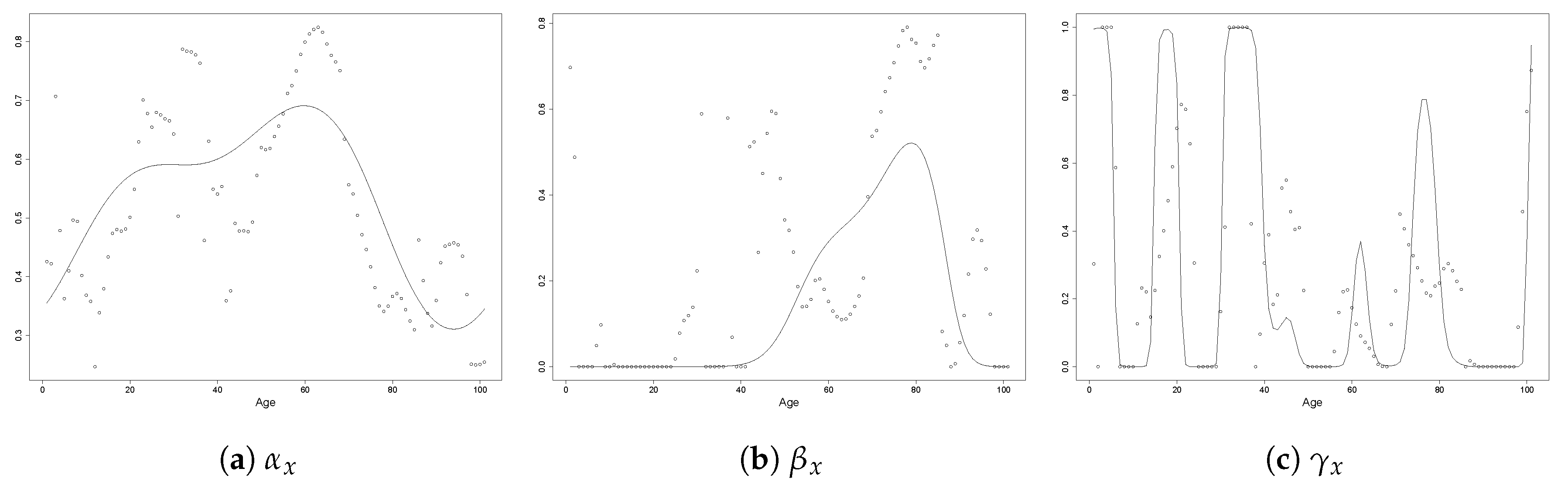
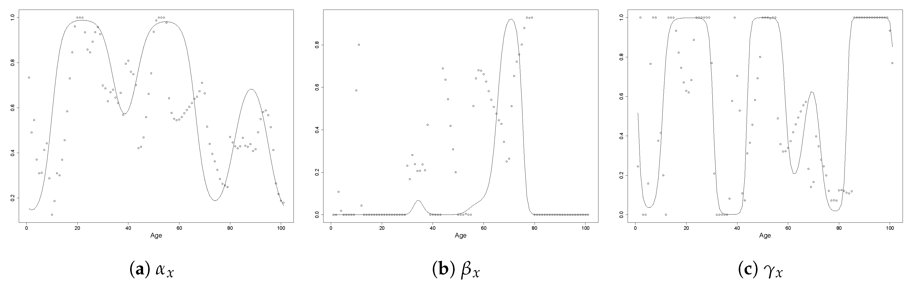
Fit an unpenalised 2-ETS model to obtain ${\widehat{\alpha }}_{x,i}$, ${\widehat{\beta }}_{x,i}$ and ${\widehat{\gamma }}_{x,i}$;

(2)

Select $n_{{\alpha }_i}$, $n_{{\beta }_i}$ and $n_{{\gamma }_i}$ as described in Section 3.2;

(3)

Given the chosen $n_{{\alpha }_i}$, $n_{{\beta }_i}$ and $n_{{\gamma }_i}$, select the tuning parameters ${\lambda }_1$ and ${\lambda }_2$ as described in Section 3.3; and

(4)

Use the selected n’s and $\lambda$’s with (15) to minimise (14).

Forecasts of mortality rates can then be produced using the model as fitted above. The associated prediction intervals (PIs), can be produced via simulations based on the multi-Gaussian errors. The ${\mathbf{\Sigma }}_{\mathit{i}}$ can be computed as the sample covariances of ${\widehat{\epsilon }}_{x,t,i}$ given the obtained estimates of parameters.

4. Empirical Analysis

We have collected mortality data of Australian female and male populations aged 0–100 between 1950 and 2016 from the Human Mortality Database (2020). The starting year is chosen as that investigated in Booth et al. (2006) and Hyndman et al. (2012) to obtain a complete and relevant dataset. Figure 3 displays the age-specific log death rates over the sample period. It can be seen that Australian Females and males both exhibit continual mortality improvements, while some distinctions exist. For example, the decrease of male death rates at around age 20 (accident hump) has been more rapid than that for females in recent years. Multi-population models may be able to capture those similarities and differences between the two populations. We compare the forecasting performance between the LC, ETS, 2-ETS, LL, and CFDM models using the 10-step-ahead projection, with a training set of 1950–2006. Then, the predictions are compared against observed (true) values to assess forecast accuracy. Female and male data are modelled separately (jointly) under the single-population (multi-population) models.

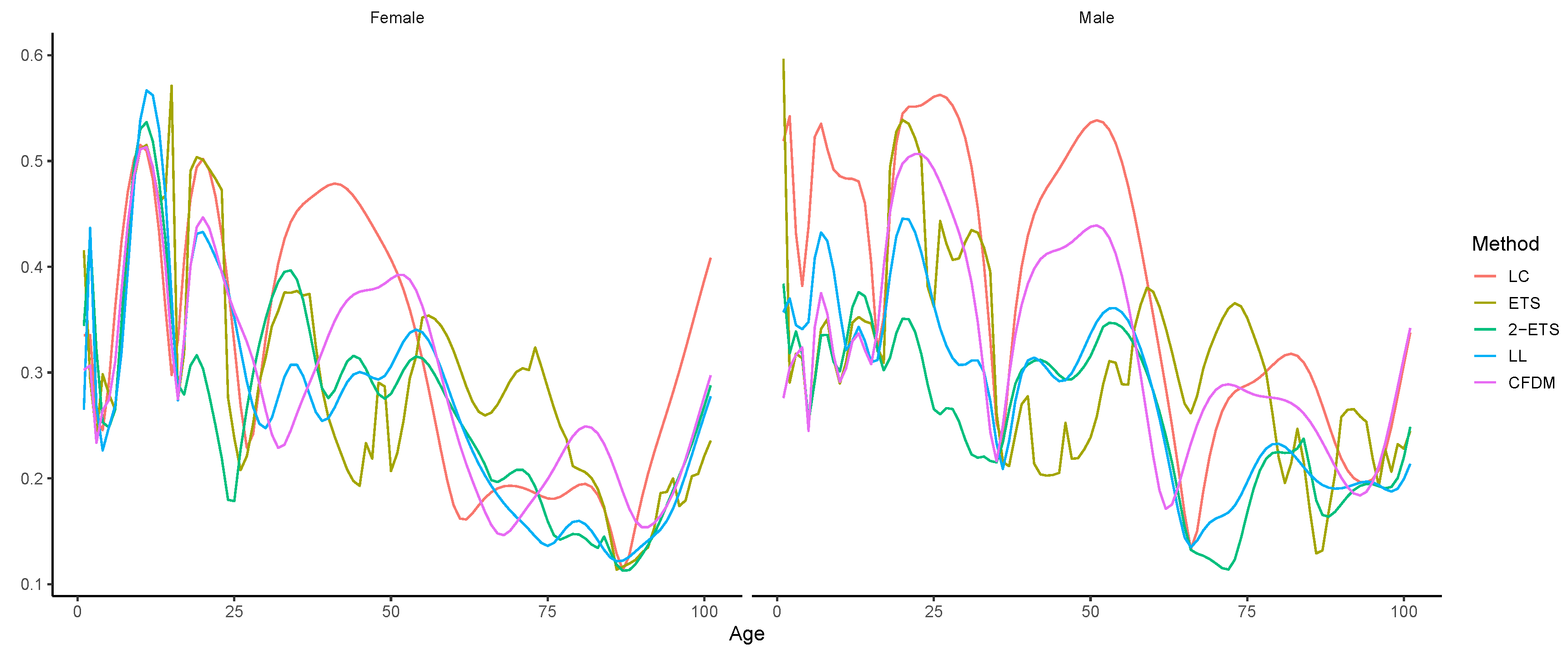
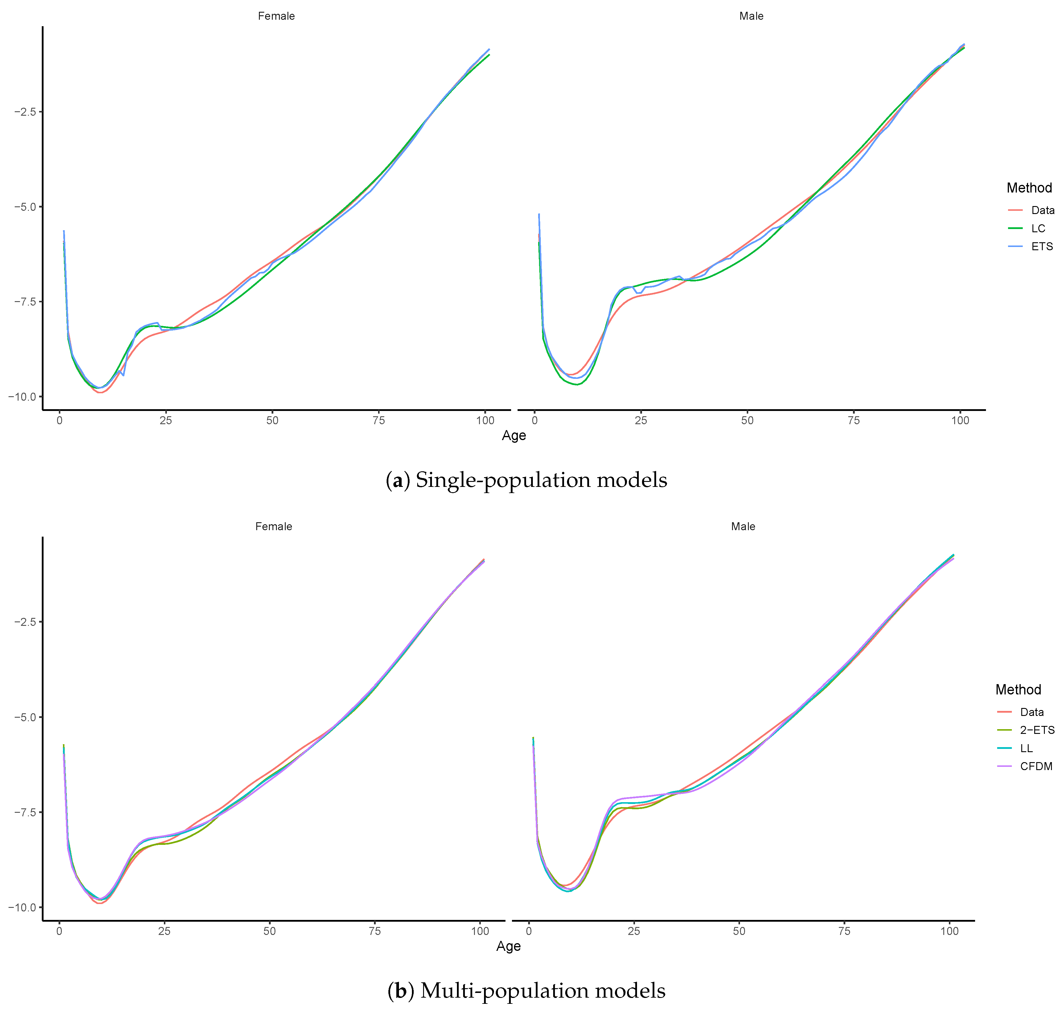
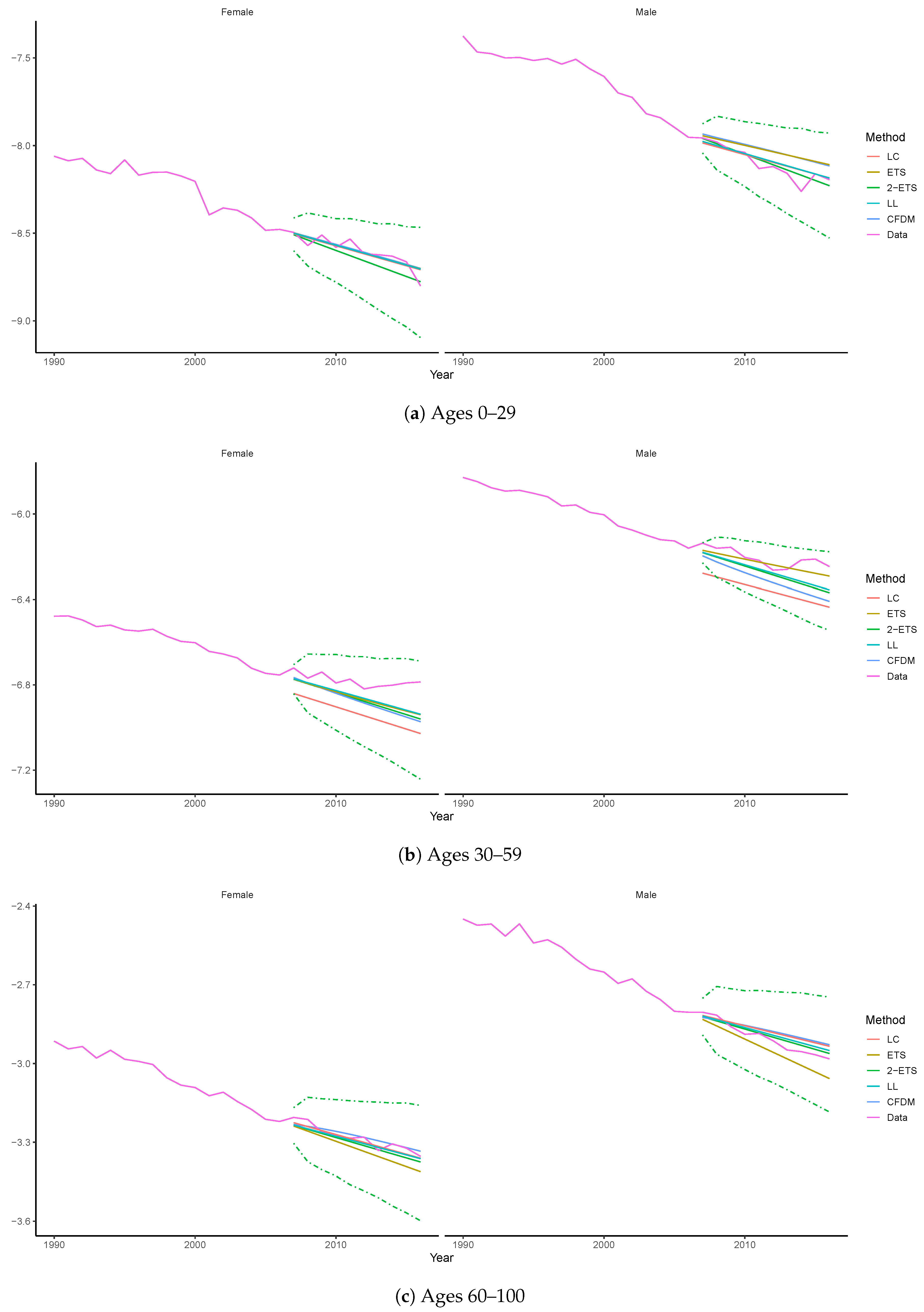
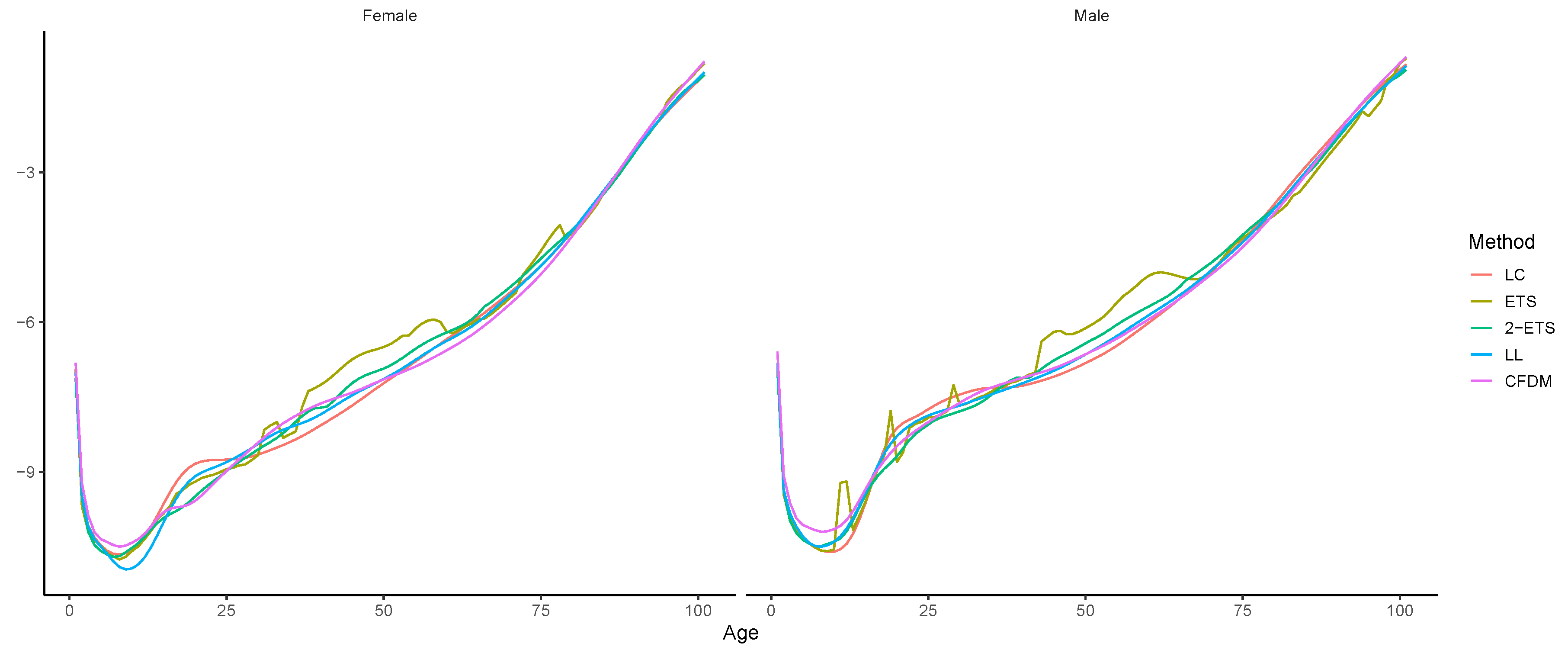
4.1. Forecast Accuracy Comparison

The forecast accuracy of the mortality models is examined by the RMSE at age x, forecasting step h and as a total measure across age groups and time horizons as follows.

$$\begin{array}{cc}\hfill RMS{E}_{x,i}& =\sqrt{\frac{1}{10}\sum _{h=1}^{10}{(ln{m}_{x,T+h,i}-ln{\widehat{m}}_{x,T+h,i})}^2}\hfill \\ \hfill RMS{E}_{h,i}& =\sqrt{\frac{1}{101}\sum _{x=0}^{100}{(ln{m}_{x,T+h,i}-ln{\widehat{m}}_{x,T+h,i})}^2}\hfill \\ \hfill RMS{E}_{all,h,i}& =\sqrt{\frac{1}{101\times h}\sum _{j=1}^h\sum _{x=0}^{100}{(ln{m}_{x,T+j,i}-ln{\widehat{m}}_{x,T+j,i})}^2}\hfill \end{array},$$

(16)

where $RMS{E}_{x,i}$ ($RMS{E}_{h,i}$) is the root mean squared error at age x (forecasting step h) across 10 prediction steps (101 ages) for population i, $RMS{E}_{all,h,i}$ is a two-dimensional criterion measuring forecast error over all age groups and time horizons up to h.

Figure 4 plots the $RMS{E}_{x,i}$ against age. A summary of RMSE values computed across ages is presented in

Table 1. Summary of RMSEs over age groups for the forecast of Australian female (Panel A) and male (Panel B) mortality.

Model	${\mathit{RMSE}}_{\mathit{all},10,\mathit{i}}$	Mean	Std. Dev.	${\mathit{Q}}_1$	${\mathit{Q}}_3$
Panel A: Female
LC	0.1383	0.1144	0.0781	0.0369	0.1846
ETS	0.1173	0.0952	0.0688	0.0448	0.1183
2-ETS	0.0994	0.0802	0.0590	0.0386	0.0980
LL	0.1059	0.0828	0.0663	0.0288	0.1015
CFDM	0.1097	0.0925	0.0592	0.0456	0.1395
Panel B: Male
LC	0.1884	0.1625	0.0957	0.0794	0.2524
ETS	0.1217	0.1031	0.0649	0.0569	0.1243
2-ETS	0.0789	0.0705	0.0356	0.0379	0.0987
LL	0.0965	0.0844	0.0472	0.0392	0.1168
CFDM	0.1291	0.1129	0.0628	0.0669	0.1658

Note: $RMS{E}_{all,10,i}$ is the overall measure across all ages and forecasting steps for population i. The columns Mean, Std. Dev., $Q_1$ and $Q_3$ display the sample mean, standard deviation, first and third quartiles of $RMS{E}_{x,i}$ calculated over age groups, respectively. The minimum value of each statistic among the five models is presented in bold.

. As indicated, the LC model tends to produce the least accuracy at most ages for both genders, whereas no single model uniformly beats the rest. More specifically, all the models except 2-ETS show some peaks (abnormally large RMSE values) at age groups of around 20 for female population, and the forecast error at around age 12 under all the five candidates present a significant peak. For males, besides the unusually large $RMSE$ at age 20, LC and CFDM exhibit a peak at age 60. In general, the two single-population models and CFDM tend to produce large RMSEs at certain ages. The curves of LL and 2-ETS show similar shapes, whereas our 2-ETS model clearly outperforms all the other competing models over ages 15–30.

One advantage of 2-ETS is that it does not produce abnormally large RMSE, which is shown by its standard deviation in Table 1, being the smallest among all the models. The first column in Table 1 gives the overall measure of the forecast accuracy. It is interesting to see that the three multi-population models outperform the two single-population models for both genders (except under CFDM for males). More specifically, the best-performing model is 2-ETS, followed by LL, and LC tends to produce the least accurate predictions. The results of ETS and CFDM are fairly close to each other, though CFDM (ETS) tends to predict female (male) population more accurately. The above relationships also hold for RMSEs averaged over age groups. In general, all the statistics except the first quartile $Q_1$ advocate the newly proposed 2-ETS model for both genders. The superiority of the 2-ETS over the rest is more obvious for males.

We now consider the prediction results over time horizons. The two-dimensional measure $RMS{E}_{all,h,i}$ against forecasting horizon h is plotted in Figure 5. Among the five candidates, LC is the worst-performing model with notably the highest forecast errors, and the differences become even more evident for Australian males. Unlike the earlier observations, the multi-population models do not consistently beat the single-population ETS. For instance, the LL curve lies above the ETS curve before a crossover at around step 5 for the two populations. Nevertheless, our 2-ETS almost consistently outperforms the other competing models, especially for males. The individual $RMS{E}_{h,i}$ values at each forecasting step are summarised in

Table 2. Summary of $RMS{E}_{h,i}$ under different forecasting horizons for Australian mortality data.

Steps	Female					Male
	LC	ETS	2-ETS	LL	CFDM	LC	ETS	2-ETS	LL	CFDM
1	0.0965	0.0647	0.0648	0.0708	0.0522	0.1368	0.0518	0.0506	0.0606	0.0622
2	0.0964	0.0662	0.0592	0.0683	0.0562	0.1546	0.0595	0.0507	0.0565	0.0588
3	0.1374	0.1038	0.0932	0.1052	0.0984	0.1632	0.0718	0.0589	0.0742	0.0774
4	0.1089	0.0790	0.0600	0.0748	0.0741	0.1981	0.1065	0.0801	0.1054	0.1026
5	0.1403	0.1097	0.1028	0.1095	0.1098	0.1642	0.0998	0.0580	0.0735	0.0743
6	0.1061	0.0817	0.0761	0.0757	0.0852	0.1653	0.1048	0.0532	0.0722	0.0681
7	0.1465	0.1343	0.1076	0.1225	0.1290	0.2139	0.1477	0.0807	0.1137	0.1047
8	0.1692	0.1580	0.1332	0.1375	0.1425	0.2178	0.1664	0.1045	0.1315	0.1321
9	0.1780	0.1693	0.1422	0.1493	0.1577	0.2241	0.1592	0.1099	0.1213	0.1189
10	0.1713	0.1468	0.1137	0.1086	0.1345	0.2205	0.1722	0.1077	0.1189	0.1170

Note: The bold numbers in each row refer to the minimum RMSE value among the five models.

. Consistent with our observations in Figure 5, the 2-ETS model produces the smallest RMSE consistently for males and leads to the 6 out of 10 minimum $RMS{E}_{h,i}$ for females.

It is worth investigating the desirable smoothness of the 2-ETS model with the empirical data. Figure 6 plots the projected and observed mortality rates for Australian females and males in 2016. The results of the single-population models are given in the top panel. The ETS curve shows more irregularities over neighbouring ages for both genders. In comparison, the predicted values under the 2-ETS model are not only much more smoothed out over neighbouring ages but also closer to the observed values. Furthermore, the LC model tends to over-estimate (under-estimate) the mortality rates for females aged 20–30 (30–60) and for males aged 20–40 (5–15 and 40–60). The multi-population models (bottom panel) seem to produce similar levels of forecasts and tend to outperform the two single-population candidates. Among the three multi-population models, 2-ETS clearly beats LL and CFDM over age range 15–30, whereas performances of the three are similar for the older populations. Overall, it can be concluded that the proposed 2-ETS model predicts the Australian mortality rates in 2016 reasonably well. The smoothness over adjacent ages is also observed.

4.2. Prediction Intervals via Simulation

We now evaluate the interval forecasts of the 2-ETS model via simulation, as briefly discussed in the end of Section 3.4. The simulation procedure is summarised as follows.

• Given the in-sample period 1950–2006, we estimate the model parameters and calculate the fitted (log) central death rates $ln{\tilde{m}}_{x,t,i}$;
• The $57\times 101$ residuals are then collected as ${\tilde{\epsilon }}_{x,t,i}=ln{m}_{x,t,i}-ln{\tilde{m}}_{x,t,i}$, which are assumed to follow a multi-Gaussian distribution with means 0 and covariance computed as sample values from using ${\tilde{\epsilon }}_{x,t,i}$;
• Given the assumed distribution, simulate a $10\times 101$ matrix of error terms, which is applied to the 2-ETS projections from 2007 to 2016, according to (12); and
• The process is repeated until 5000 replicates are produced.

Figure 7 plots the observed and predicted values of log mortality rates averaged over different age groups. The green solid line refers to the point forecasts under the 2-ETS model. The associated 95% PIs obtained via simulations are presented as dashed lines. It can been seen that over 2007–2016, the observed values consistently fall within those PIs for both females and males. Nevertheless, the projections under the five models are not far away from one another, except for the middle age group under the LC model.

To sum up, with a 10-year out-of-sample period, we demonstrated the outperformance of the proposed 2-ETS model over the existing models. Its smoothness is also present in the scenario of $h=10$ (2016). In the next section, we further explore the coherence and smoothness of the 2-ETS from a long-term forecasting perspective, and compare its performance with the other four competing models.

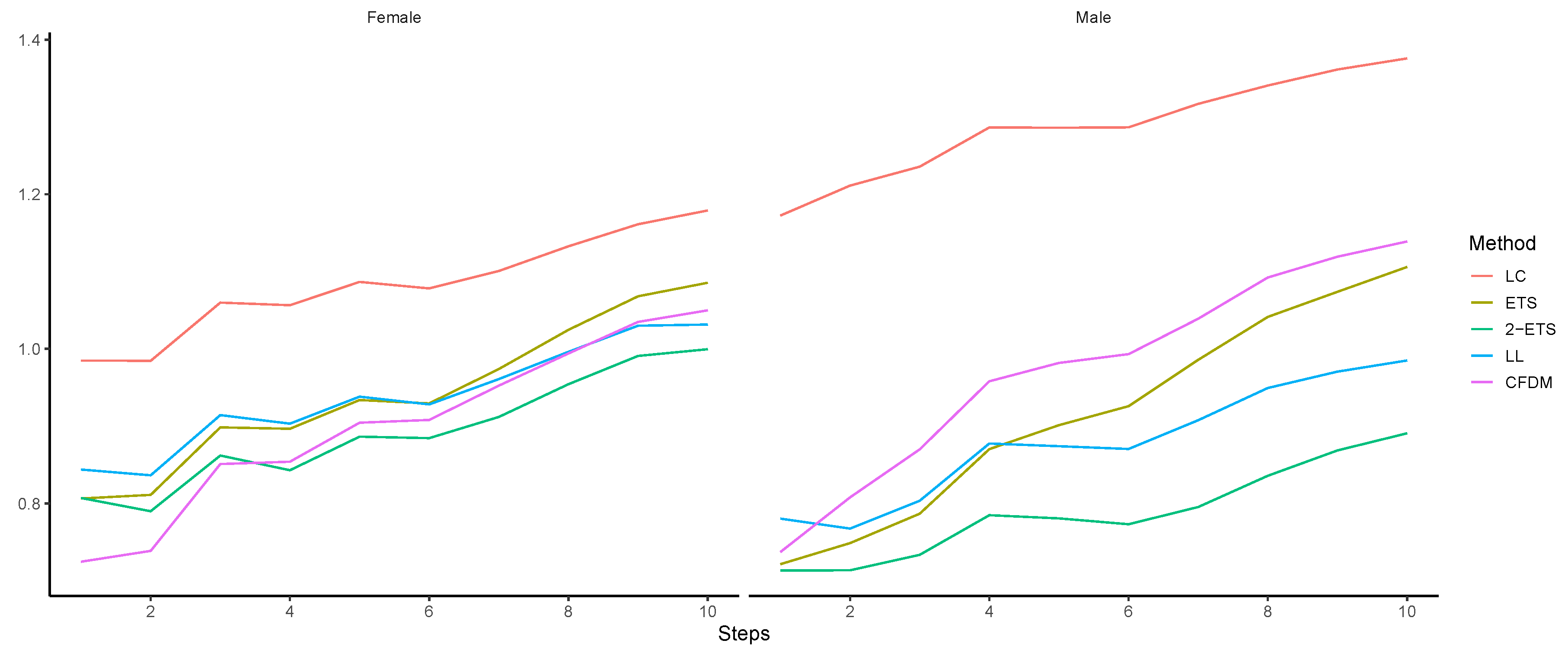
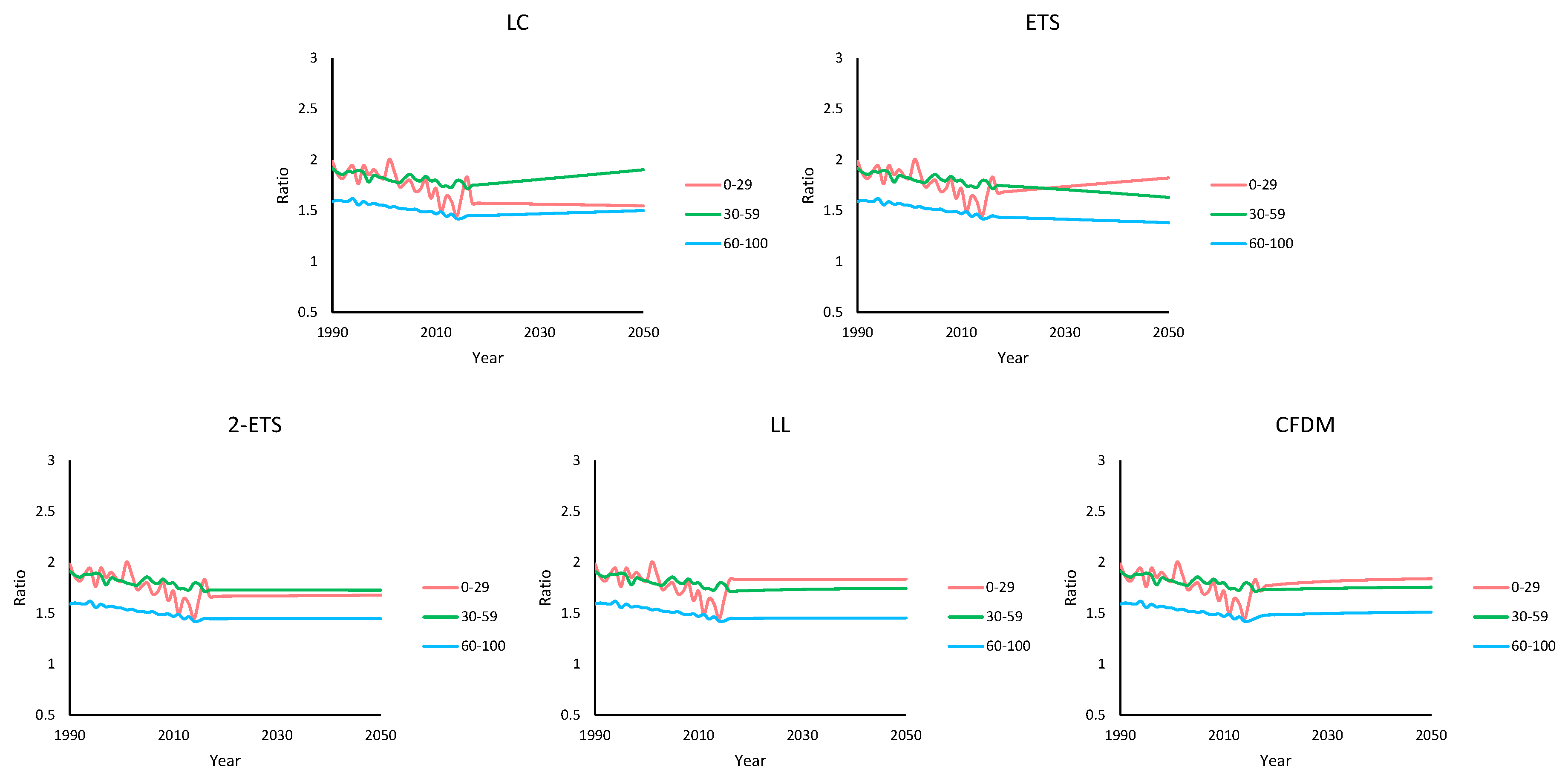
4.3. Long-Term Forecasting Performance

To investigate the long-term performance of the five candidates, we obtained projections up to 2050 based on the full sample (1950–2016). The results are plotted in Figure 8. The curves of the two single-population models exhibit some deviations from those of the multi-population counterparts. Firstly, under the LC model, there is a significant accident hump in 2050 for female population only. Forecast curves of the other models do not have such a deep hump. Furthermore, female mortality improvements forecasted by the LC tend to be smaller than those produced by the multi-population models over ages 30–60. This is less evident when males data are analysed. When the ETS model is adopted, as expected and being consistent with Figure 6, significant irregularities over neighbouring ages are evident for both genders. Such irregularities are not observed in the case of 2-ETS model, indicating its improved smoothness across ages. Among the three multi-population candidates, CFDM tends to produce the lowest (highest) rates for the youngest (oldest) 15-year age group for both genders. The 2-ETS curve lies above the other two over age range 40–80. Apart from that, some sex-specific differences are also present. For example, the predicted mortality rates under LL for Australian females aged 5–15 are much lower than those of 2-ETS and CFDM.

Following Li (2013), we examine the coherence of mortality forecasts between sexes by plotting the male-to-female ratios from 1990 to 2050. The observed (predicted) mortality rates are averaged over each of the three age groups: 0–29, 30–59, and 60–100, then the mean values of the male population are divided by those of the female population to obtain the corresponding ratios. As indicated in Figure 9, the three multi-population models produce convergent ratios in the long run for all age intervals, which is not the case when single-population models are applied. For instance, the male-to-female ratios of the youngest group under the LC model and the middle age group under the ETS model show a decreasing trend, which potentially causes the crossover problem of mortality forecasts between genders.

In conclusion, without considering coherence between populations and smoothness across ages, single-population models would perform differently from multi-population models in the long-run. In particular, the single-population ETS model produces undesirable divergent mortality forecasts, which can be largely avoided when the 2-ETS model is employed. Considering the results discussed in Section 4.1 and Section 4.2, we can conclude that the 2-ETS model is the best performing model which also effectively achieves coherence and smoothness, when the Australian female and male mortality data are examined.

5. Conclusions

This research proposes a 2-ETS model with smoothing penalisation scheme and demonstrates its coherence property in mortality forecasting. Using an effective dimensionality reduction technique, we evaluate the out-of-sample forecasting accuracy of 2-ETS based on the Australian female and male mortality data. Two single-population models LC and ETS, and two multi-population models LL and CFDM are also tested and compared with the proposed candidate. Our analysis demonstrates that the 2-ETS model tends to produce less large forecast errors at different age groups (measured by RMSEs) when compared to the other candidates. For different forecasting horizons, the 2-ETS model almost consistently leads to smaller forecast errors than the others, especially for Australian males. The superiority of our proposed model is further demonstrated by the overall accuracy measure considering both age and time dimensions. We then construct the associated PIs via a simulation study based on the multivariate Gaussian assumption of error terms. In general, the multi-population models tend to outperform the single-population candidates regarding prediction accuracy. Although the original ETS model produces satisfactory RMSEs, it suffers from a shortcoming of fluctuating forecasts across adjacent ages and divergent forecasts between genders. From the 10-step-ahead and long-term projections, we can observe that the proposed 2-ETS model overcomes the above problems. Mortality forecasts under the new model are coherent between males and females in the long run and are smoothed over neighbouring ages.

There are several directions for future study. Firstly, the 2-ETS model may be extended to cater for co-modelling of three or more sub-populations of a group in practice. For example, the joint projection of state-level data would be useful for government planning such as social benefits and superannuations. Secondly, the model may be applied or modified to investigate the evolution of age patterns in mortality data by fixing the time effect and forecast in the age dimension. Moreover, the ETS specification does not consider mortality improvements linked to the year of birth. Either a common or population-specific cohort factor may be added to the model structure, but further research is needed. Other approaches to identify parameter estimates and to reduce the dimensionality may also be performed in future research.

References

1. Booth, Heather, Rob Hyndman, Leonie Tickle, and Piet De Jong. 2006. Lee-Carter mortality forecasting: A multi-country comparison of variants and extensions. Demographic Research 15: 289–310. [Google Scholar] [CrossRef]
2. Feng, Lingbing, and Yanlin Shi. 2018. Forecasting mortality rates: Multivariate or univariate models? Journal of Population Research 35: 289–318. [Google Scholar] [CrossRef]
3. Gardner, Everette S., Jr. 1985. Exponential smoothing: The state of the art. Journal of Forecasting 4: 1–28. [Google Scholar] [CrossRef]
4. Gardner, Everette S., Jr., and Ed. McKenzie. 1985. Forecasting trends in time series. Management Science 31: 1237–46. [Google Scholar] [CrossRef]
5. Giacometti, Rosella, Marida Bertocchi, Svetlozar Rachev, and Frank Fabozzi. 2012. A comparison of the Lee–Carter model and AR–ARCH model for forecasting mortality rates. Insurance: Mathematics and Economics 50: 85–93. [Google Scholar] [CrossRef]
6. Human Mortality Database. 2020. University of California, Berkeley (USA), and Max Planck Institute for Demographic Research (Germany). Available online: www.mortality.org (accessed on 23 March 2020).
7. Hyndman, Rob, Heather Booth, and Farah Yasmeen. 2012. Coherent mortality forecasting: The product-ratio method with functional time series models. Demography 50: 261–83. [Google Scholar] [CrossRef] [PubMed] [Green Version]
8. Hyndman, Rob, and Yeasmin Khandakar. 2008. Automatic time series forecasting: The forecast package for r. Journal of Statistical Software 26. [Google Scholar] [CrossRef] [Green Version]
9. Hyndman, Rob, Anne B. Koehler, J. Keith Ord, and Ralph D. Snyder. 2008. Forecasting with Exponential Smoothing: The State Space Approach. Springer Series in Statistics; Berlin and Heidelberg: Springer. [Google Scholar]
10. Hyndman, Rob, Anne Koehler, Ralph Snyder, and Simone Grose. 2002. A state space framework for automatic forecasting using exponential smoothing methods. International Journal of Forecasting 18: 439–54. [Google Scholar] [CrossRef] [Green Version]
11. Hyndman, Rob, and Md. Shahid Ullah. 2007. Robust forecasting of mortality and fertility rates: A functional data approach. Computational Statistics and Data Analysis 51: 4942–56. [Google Scholar] [CrossRef] [Green Version]
12. Hyndman, Rob J., and George Athanasopoulos. 2018. Forecasting: Principles and Practice. Melbourne: OTexts. [Google Scholar]
13. Hyndman, Rob J., Anne B. Koehler, J. Keith Ord, and Ralph D. Snyder. 2005. Prediction intervals for exponential smoothing using two new classes of state space models. Journal of Forecasting 24: 17–37. [Google Scholar] [CrossRef]
14. Hyndman, Rob J., and Han Lin Shang. 2009. Forecasting functional time series. Journal of the Korean Statistical Society 38: 199–211. [Google Scholar] [CrossRef]
15. Lee, Ronald, and Timothy Miller. 2001. Evaluating the performance of the lee-carter method for forecasting mortality. Demography 38: 537–49. [Google Scholar] [CrossRef]
16. Lee, Ronald D., and Lawrence R. Carter. 1992. Modeling and forecasting U.S. mortality. Journal of the American Statistical Association 87: 659–71. [Google Scholar] [CrossRef]
17. Li, Hong, and Yang Lu. 2017. Coherent forecasting of mortality rates: A sparse vector-autoregression approach. ASTIN Bulletin: The Journal of the IAA 47: 563–600. [Google Scholar] [CrossRef]
18. Li, Jackie. 2013. A poisson common factor model for projecting mortality and life expectancy jointly for females and males. Population Studies 67: 111–26. [Google Scholar] [CrossRef]
19. Li, Nan, and Ronald Lee. 2005. Coherent mortality forecasts for a group of populations: An extension of the lee-carter method. Demography 42: 575–94. [Google Scholar] [CrossRef] [Green Version]
20. Makridakis, Spyros, and Michele Hibon. 2000. The m3-competition: Results, conclusions and implications. International Journal of Forecasting 16: 451–76. [Google Scholar] [CrossRef]
21. Pegels, C. Carl. 1969. Exponential forecasting: Some new variations. Management Science 15: 311–15. [Google Scholar]
22. Renshaw, Arthur E., and Steven Haberman. 2003. Lee–carter mortality forecasting with age-specific enhancement. Insurance: Mathematics and Economics 33: 255–72. [Google Scholar] [CrossRef]
23. Renshaw, Arthur E., and Steven Haberman. 2006. A cohort-based extension to the Lee-Carter model for mortality reduction factors. Insurance: Mathematics and Economics 38: 556–70. [Google Scholar] [CrossRef]
24. Taylor, James W. 2003. Exponential smoothing with a damped multiplicative trend. International Journal of Forecasting 19: 715–725. [Google Scholar] [CrossRef] [Green Version]
25. Wong, Kenneth, Jackie Li, and Sixian Tang. 2020. A modified common factor model for modelling mortality jointly for both sexes. Journal of Population Research 37: 1–32. [Google Scholar] [CrossRef]
1
See Hyndman et al. (2002) for a thorough review of exponential smoothing methods.
2
A maximum likelihood method may also be employed to calibrate the parameters (Renshaw and Haberman 2003).
3
In our preliminary analysis, all damped parameters essentially approach 1 after a penalised structure is considered as in (14).
4
In contrast to Li and Lu (2017), we do not penalise α x , i , β x , i and γ x , i . One reason is that those parameters will be smoothed after applying the procedure described in Section 3.2. The other reason is that out-of-sample forecasts of ln m x , t , i do not directly depend on them. In other words, smoothed parameters will not necessarily enforce the smoothness of b x , T , i across x.
Figure 1. Estimated α x , β x and γ x for Australian female mortality data.
Risks 08 00067 g001
Figure 2. Estimated α x , β x and γ x for Australian male mortality data.
Risks 08 00067 g002
Figure 3. Log mortality rates for Australian population 1950–2016.
Risks 08 00067 g003
Figure 4. R M S E x , i plotted against age groups for Australian mortality data.
Risks 08 00067 g004
Figure 5. R M S E a l l , h , i plotted against forecasting horizon h for Australian mortality data.
Risks 08 00067 g005
Figure 6. Predicted vs actual log mortality rates for Australia in 2016.
Risks 08 00067 g006
Figure 7. Predicted vs actual log mortality rates (averaged over different age groups) for Australia: 1990–2016. Note: Solid lines display forecast and actual mortality rates averaged over all ages, and dashed lines are the PIs produced under the 2-ETS model.
Risks 08 00067 g007
Figure 8. Predicted log mortality rates for Australia in 2050.
Risks 08 00067 g008
Figure 9. Observed and projected male-to-female ratios of mortality rates for Australia.
Risks 08 00067 g009