Abstract
In a one price economy, the Fundamental Theorem of Asset Pricing (FTAP) establishes that no-arbitrage is equivalent to the existence of an equivalent martingale measure. Such an equivalent measure can be derived as the normal unit vector of the hyperplane that separates the attainable gain subspace and the convex cone representing arbitrage opportunities. However, in two-price financial models (where there is a bid–ask price spread), the set of attainable gains is not a subspace anymore. We use convex optimization, and the conic property of this region to characterize the “no-arbitrage” principle in financial models with the bid–ask price spread present. This characterization will lead us to the generation of a set of price factor random variables. Under such a set, we can find the lower and upper bounds (supper-hedging and sub-hedging bounds) for the price of any future cash flow. We will show that for any given cash flow, for which the price is outside the above range, we can build a trading strategy that provides one with an arbitrage opportunity. We will generalize this structure to any two-price finite-period financial model.
1. Introduction
It has been known for a long time (Harrison and Kreps 1979; Harrison and Pliska 1981; Delbaen and Schachermayer 1994) that no-arbitrage opportunity in a one price economy is equivalent to the existence of an equivalent martingale measure. This result is usually referred to as the Fundamental Theorem of Asset Pricing (FTAP). Rogers (1994) used a directional derivative argument to provide a discrete-time proof for FTAP. The case of trading continuously, in particular, was discussed by Harrison and Pliska (1981).
In practice, the law of one price often does not hold. Recently, the literature on transaction costs and the study of no-arbitrage in the presence of bid–ask spreads has been expanding (Jouini and Kallal 1995; Bion-Nadal 2009; Guasoni et al. 2011). Madan (2012) considers financial equilibrium where there are two separate prices at which one may buy from or sell to the market known as ask and bid prices. This is a realistic situation in financial markets. Inside an efficient market, at a given time, a financial security trades at a unique price. The equilibrium conditions that are needed to provide a unique price all depend on arbitrage opportunities that are quickly exploited. A wide category of financial securities trade in vast and diverse markets and few of them meet the equilibrium conditions we mentioned earlier. Market clearing becomes troubling, which leads to prices that are not unique for equivalent securities in different markets. Whenever the above conditions are not satisfied, the “law of one price“ fails to hold. On the other hand, an incomplete market can also take place even under the assumption of “one price”. Incomplete condition explains that there exists the presence of some residual risks that can not be eliminated regardless of the existence of the best hedging (Eberlein et al. 2009; Jacka 1992). In addition, the markets establish a phenomenon that is not anticipated in the one price theory called illiquidity. Illiquidity can be explained as the lack of ability of the market to establish a unique price, that is, to eliminate the spread between the bid and ask prices. This happens when there is an absence of information and/or a lack of interested parties. In these situations, the bid and ask prices are the only real market information that can be observed. Thus, the theoretical framework that has been used to explain the one price market is not accurate enough to deal with many situations one faces in practice.
We adopt the framework of “conic finance“ in this paper. Some earlier studies that use the theory of conic finance include Madan (2012); Cherny and Madan (2010); Eberlein and Madan (2009, 2012); Eberlein et al. (2011). The direction of trade is what distinguishes the theory of two-price economies from that of one price economy. Now there are two types of prices, one price is used for buying from the market called the ask price, and the other price is used for selling to the market called the bid price. In the situation of one price economy, the market plays the role of an auctioneer, who clears the trades and decides the prices. However, in the two-price economy, the financial market plays a role of a passive counterparty to all transactions, who buys at the ask price and sells at the bid price. The spread that is between the bid and ask prices becomes a measure of illiquidity. It also evaluates the principal required to support a position and the cost of unraveling a position.
We also find it necessary to mention that the one-period case discussed in this paper was included in the book by Carr and Zhu (2018) with reference to this paper (a working paper back then).
1.1. Bid–Ask Spreads
A collection of theoretical approaches exists that are trying to model bid–ask spreads. Cherny and Madan (2010) offer a few of the current approaches that have been used to model bid–ask spreads. Copeland and Galai (1983) have discussed the order processing and inventory costs of providers of liquidity. Constantinides (1986) and Jouini and Kallal (1995) investigated the spreads that involve transaction costs of trading in liquid markets. However, the researches mentioned above are comparatively satisfactory to liquid markets where a transaction cost can happen at a price that a contrary trade direction can take place with no price effect. The price-spreads that are related to the theory of two-price economies are discussed in Carr et al. (2001) and Cherny and Madan (2010). These are mostly related to locating actual long-term counterparties that are ready to establish a position for an extended period of time. The spread between the bid and ask prices can be observed as a holding of the charge-exerted while the market does not clear rapidly, as to find a counterparty is going to require time and effort because there is no possibility of doing trades in both directions at any transaction price being observed. Specifically, there is not any possibility of complete replication. In addition, the spread between the bid and ask prices becomes a reflection of the cost of holding the residual risk (Eberlein et al. 2011). Therefore, transactions happen close to or at either the ask price or the bid price, conditional on the direction of the trade. The conic finance is trying to model the bid–ask spread by applying the concept of acceptable cash flows to the market (Madan 2015). However, it is assumed that the market requires a minimal level of acceptability for a position to be profitable. As a result of the market competition, the bid-price is being raised, and the asked-price is being lowered to establish an acceptable position. Therefore the bid–ask spread is tried to be narrowed so that the risk of a position will be minimized. This spread can be seen as the cost of unraveling a position.
1.2. Two-Price Economy
In a two-price economy, a comparatively classical view of markets consistent with its role in the traditional competitive breakdown, where markets play the role of counterparties to transactions, is being assumed. The only difference from the traditional aspect is that the length of a trade depends on the direction of the trade, while the market is buying at the bid price and selling at the ask price. Now regard the classical market when trading is performed in either direction at the current price. The market is always willing to sell at a higher price or similarly buy at a lower price and welcomes all zero-cost random cash streams that have a positive expectation under the equilibrium pricing essentials. Notice that this creates a very large set of market risks that are accepted by the classical financial market within a risk-neutral measure. The two-price financial market is more antagonistic as to which trades it will accept. The collection of zero-cost risks acceptable to the financial market is much smaller as a set. A modeling process of this set of acceptable risks can be observed at Artzner et al. (1999), that was further expanded in Cherny and Madan (2009) and Cherny and Madan (2010). Especially, the set of zero-cost risks that are acceptable to the financial market as a set of random variables is being modeled as a convex cone, including all the non-negative random variables. The theoretical structure required for supporting the two-price economy has been given a huge amount of attention in the past few years. The theory was popularized into the field of mathematical finance by Constantinides (1986) and was introduced as coherent risk measures by Artzner et al. (1999). The research that connects the theory of two-price economies to concave distortions was performed by Cherny and Madan (2009) and Cherny and Madan (2010). They are the researches that gave a perceptive of how to establish the bid–ask prices admissible to the theory of two-prices. After that, the theory of two-prices was given the name “conic finance”, for example Madan and Schoutens (2011) and Madan and Schoutens (2012). In the following sections, we present the theory of two-prices in an abstract manner as it was set out in Madan (2015).
The rest of this paper is structured as follows. In Section 2 we introduce the model, starting by definitions of sets of zero cost and attainable cash flows. We also characterize the utility maximization of trading cash flows. In Section 3 the Fundamental Theorem of Asset Pricing in conic finance (two-price economy) will be stated and proved (all proofs will be in Appendix A), using the pricing factor generated by a solution of the dual problem. In Section 4 we use take advantage of the existence of pricing factors and define price bounds for any attainable cash flow. Additionally, in concrete examples, we will illustrate the trading strategies in the presence of arbitrage opportunities for 1 and 2-period models, along with the super-hedging theorem for the 1-period case. In Lemma 1 a computation complexity will be given, in presence of all possible zero cost bonds. Finally in Section 5 the multi-period case will be discussed where only the one-period bonds and assets will be considered through an iterative process.
2. The Model (Multi-Period)
In this section, we first define the general multi-period model along with all of the necessary components of the model. We establish the FTAP theorem for the multi-period model in conic finance (two-price economy) by considering a utility maximization problem and its dual. We also explain the relation between solutions to our primal and dual problems, along with the price factors derived from the solution of the dual problem, by considering a utility maximization problem and its dual. We use this price factor to find a super-hedging and sub-hedging for any acceptable cash flow.
2.1. The Model Definitions
We start by defining the general model and its components following Madan (2015).
Definition 1.
Let be an information filtration on the probability space where is a finite sample space, representing the economic states. We consider a T-period financial model where and for any , cash flows (in∖out) are being traded at time t.
Definition 2.
Let denote the space of all -adapted cash flows with the inner product
Then is a finite dimensional Hilbert space.
The market consists of M risky assets and T risk-free zero coupon bonds where and for . At time t, there is a bid and ask price pair . Paying , one will receive the income flow and receiving one will get the income flow . For risk-less bonds, the bid and ask prices of , paid/received at time is denoted by . There are two zero cost cash flows associated with each pair of bid and ask prices.
and
Similarly the bond maturing at time u, creates two zero cost cash flows as below:
and
2.2. Set of Zero-Cost Cash Flows
Assuming that one can trade any non-negative multiple of above zero-cost cash flows, and suppose are non-negative -adapted random variables, then is defined to be the set of all zero cost cash flows of the form
It can be seen from the definition that is a cone. Define to be the set of all cash flows such that there is with . Then is the set of adapted processes, super-replicable at zero cost. It is clear that a closed convex cone and .
Figure 1 is a geometrical demonstration (in ) of a cone and the convex cone , set of all vectors dominated by some elements of ().
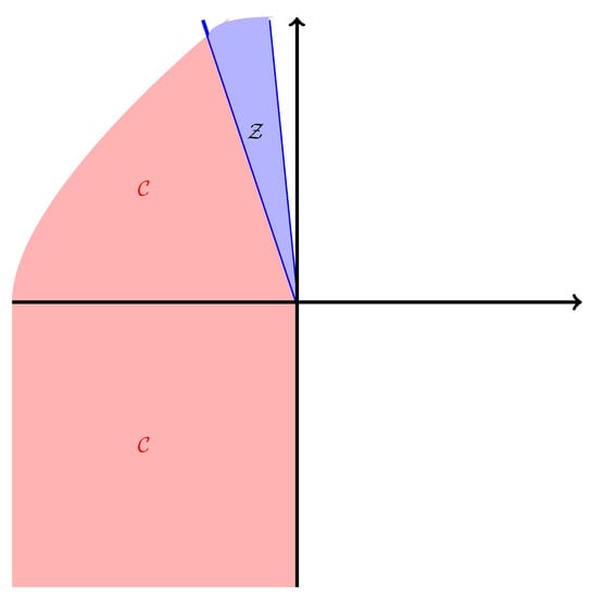
Figure 1.
Set of zero-cost cash flows , and the cone .
2.3. The Characterization of No-Arbitrage
We now define arbitrage and will be characterizing no-arbitrage using a utility maximization problem.
Definition 3.
We say that a cash flow is an arbitrage if for all .
Definition 4.
(Utility Function) An extended real valued function is called a utility function if it satisfies the following three characteristics:
- (1)
- (Risk Aversion) u is strictly concave,
- (2)
- (Profit Seeking) u is strictly increasing and ,
- (3)
- (Bankruptcy Forbidden) for any .
Let denote the non-negative cone in , also be the initial endowment and be a cash flow. Consider the following optimal trading problem
where u is a utility function. We are able to characterize the no-arbitrage principle in terms of this utility maximization problem.
Theorem 1
(Characterization of Utility Maximization). The financial market has no-arbitrage opportunity if and only if the optimal trading problem above has a finite value .
Proof.
In Appendix A. □
3. FTAP for Multi-Period Model
In this section, we establish FTAP for conic finance model, characterizing no-arbitrage in terms of the extension of pricing factors. A first version of this theorem was proven by Harrison and Kreps (1979). More general versions of the theorem were proven in 1981 by Harrison and Pliska (1981) and in 1994 by Delbaen and Schachermayer (1994).
Theorem 2
(The First Fundamental Theorem of Asset Pricing). A financial market with time horizon T and price processes of the risky asset and risk-less bond given by and , respectively, is arbitrage-free under the probability P if and only if there exists another probability measure Q such that
i. For any event A, if and only if (We say in this case that P and P are equivalent probability measures).
ii. The discounted price process, is a martingale under Q. A measure Q that satisfies (i) and (ii) is known as a risk neutral measure.
We now start by considering dual of the utility maximization problem in Section 2. First, we rephrase the utility maximization problem in Section 2 as an abstract convex programming problem.
For , define and . Then we can rewrite the optimal trading problem in Equation (1) as
The dual representation of the problem above gives us an extension of the Fundamental Theorem of Asset Pricing (FTAP) in conic finance. We approach FTAP via a utility optimization problem.
Definition 5
(Pricing Factor). For , we say is a pricing factor from time t to time u and compatible with financial market, if the two following conditions are satisfied
and also for
Theorem 3.
(FTAP in conic finance) Let be a utility function and consider a two-price financial market consisting of price processes of the risky assets and risk-free bonds. Then the market is arbitrage-free under the probability P if and only if there exists a pricing factor.
Proof.
In Appendix A. □
Remark 1.
Through the proof of Theorem 3, there are a few things we would like to point out here:
- (1)
- Pricing factor is not unique. This is clear since the existence of a pricing factor in FTAP comes from the existence of a solution to the dual problem, and we know the dual problem does not necessary have a unique solution.
- (2)
- The pricing factor is related to the utility function u via the duality. In fact we saw specifically that .
- (3)
- The pricing factors can be used to generate prices for cash flows with no-arbitrage existing. We will explain this more in detail on the coming sub-section.
4. Price Bounds and Their Estimates
A distinct feature of conic finance is that prices of assets are not unique. In fact, we see that every price factor will provide a non-arbitrage price. We will see that the set of price factors will provide us price bounds, outside of which arbitrage arises.
4.1. Definition of the Bounds
Define to be the set of all price factors that are compatible with the financial market which is
Let . We define
and
Remark 2.
The values of and are the lower and upper bounds for bid and ask prices of the cash flow , equivalent to existing no-arbitrage. Equivalently, is the no-arbitrage region for the price of a given cash flow
Remark 3.
As we know, any of has a one to one correspondence relation to a solution of the dual problem say so that , where Q is a P-equivalent martingale measure defined as . Since are in direct relation to the solution of dual problem, this leads to
which is a linear combination in terms of the pricing factor we defined above, so that the corresponding maximization and minimization above (and later in our text) becomes a linear programming problem.
A question that one can ask is, if the market (bid and ask) prices of a cash flow , are outside of the no-arbitrage region , will any arbitrage opportunity become possible? We will answer this question in the next section.
4.2. Computations in One-Period
To illustrate the general pattern, we start with a simple example.
Example 1.
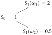
Consider a one-period model () with a sample space containing only two elements and let (only one risky asset, ). Additionally, consider a bond
where the ask and prices are and , respectively. Assume the asset over times has standard initial price 1 and payoff as following

Now consider the following primal maximization problem
A systematical way of deriving the arbitrage strategy is to use linear programming duality. By using the linear programming duality, we can write the dual problem to Equation (7) as
If we use the constraint condition in Equation (8) and substitute in the objective function, we have
but since minimum happens when so that
Therefore 1.8 is the highest ask price for offered at time under no-arbitrage condition. That means for any offered price higher than 1.8 one should be able to build a portfolio creating an arbitrage.
In fact for a bid price , since the solution to Equation (8) is , one can buy 2 unites of bond at time for the price of 1.8 and receive 2 at time so that can be delivered and still making a profit of .
Similarly we can find a lowest bid price for which one can construct a portfolio providing arbitrage if any ask price lower than is available.
The approach illustrated above can also be used in financial market that involves both bonds and stocks. A general result is summarized in the following theorem. We will use the set of all possible pricing factors corresponding to all solutions of the dual problem to provide a no-arbitrage region for a given cash flow. We state the result for super-hedging, i.e., upper bound for no-arbitrage. Sub-hedging can be discussed similarly.
Theorem 4
(Super-Hedging). Suppose that is an acceptable cash flow, then
is a super-hedging bound, where
If is a bid price that exceeds a super-hedging bound , then the solution to the minimization problem (dual) is a trading strategy for which if we acquire the zero cost cash flows , then our portfolio has an arbitrage opportunity.
Proof.
In Appendix A. □
We can see that a super-hedging bound can be represented as the value of a pair of dual linear programming problems. The primal provides an easy way of evaluating with the help of price factor in set . The dual solution, provides us a super-hedging portfolio which guarantees an arbitrage in case of existence of a favorable price for the cash flow
4.3. Two-Period Examples
Before we start setting up the problem for a two-period model, first we aim to explain a simple example for a two-period case. We will discuss and illustrate this two-period model with only one risky asset.
4.3.1. Involving Only 1-Period Bonds
Example 2.
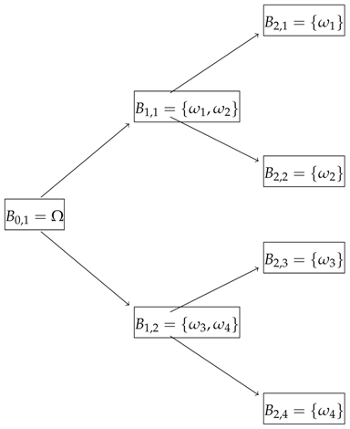
Let and consider a two-period model with and and the information structure where for , the σ-algebra is generated by the set which are defined as . The sets are all subsets of Ω and they are defined as in the following diagram


Additionally, consider the bonds
where and also .
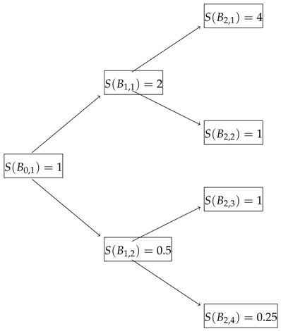
Let be our only risky asset with the above price diagram corresponding to zero-cost cash flows
We aim to find the highest ask price while no-arbitrage exists. We need to mention here that we are assuming there is no 2-period bond is available. We are going to treat the problem as two consecutive 1-period problems. For this reason, first we try to find the best ask price (a -measurable random variable) of having being paid at time . Therefore for we construct the following maximization problem
and by definition 2.2 we have
for which the Lagrangian becomes
so that we have
or
Solving the latter linear programing we will have:
Now consider the following diagram and maximization problem
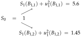

Similar to example (1), this problem has the solution
Therefore 3.42 is the highest ask price for ) offered at time to have the no-arbitrage condition satisfied. That means for any offered price bigger than 3.42 one should be able to build a portfolio creating an arbitrage.
In fact for an offered bid price of , since the dual problem solutions are , one can buy 5.6 unites of bond at time for the price of 3.42 and receive 5.6 at time so that can be delivered and left with at least so that one is able to deliver at time and still making a profit of at least .
Similarly we can find a lowest bid price for which one can construct a portfolio providing an arbitrage if any ask price smaller than is available, where analogous steps to example (1) leads to
Therefore 0.6525 is the lowest bid price (sub-hedging bound) for offered at time to have the no-arbitrage condition satisfied. That means for any offered ask smaller than 0.6525 one should be able to build a portfolio creating an arbitrage.
Next, we consider a problem involving options using a similar approach.
Example 3.
Let and consider a two-period model with the information structure where for , the σ-algebra is generated by the set which are defined as . The sets are all subsets of Ω and they are defined as in the following diagram
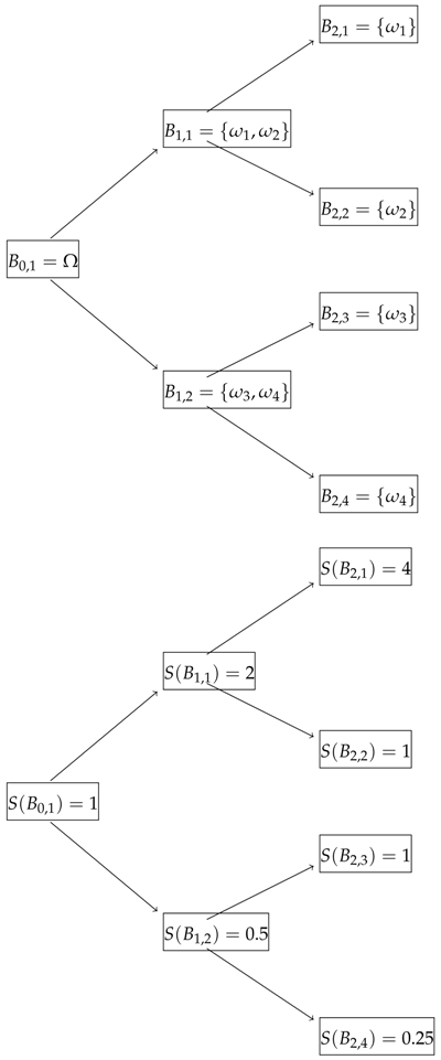

We define the risk-free bonds as
where and also . Let be our only risky asset with the above price diagram with zero-cost cash flows
and also according to our calculations in the previous example
Now consider an option with the payoff of at times and as the underlying asset. Additionally, assume the strike price of at time . Then the payoffs are .
Consider the cash flow . We would like to find the highest ask-price at time for this cash flow. Therefore we consider the following maximization problem
On the other hand, we know that
Therefore, similar to our previous example, first we find a super-hedging bound for (the random variable ), at time . Since is a random variable taking value on and , for which corresponds to the two sub-branches of the diagram at time , we set up a linear programming maximization as
which has the values of and .
Now that we have values determined and since , we use the following problem to calculate
which has the maximum value of .
Now if at time there is an available cash flow with , then one can use the following zero-cost trading strategy to create an arbitrage. In fact the arbitrage strategy is to invest all of amount into at time and then invest the revenue received at time into , therefore at time one will have
so that an arbitrage is available.
Again, we can find the lowest bid-price at time for the cash flow as
and this is the lowest bid price possible under no-arbitrage condition. Now, if at time there is a cash flow available where , then one should be able to have an arbitrage. In fact, by constructing the following zero-cost trading strategy, that is shorting units of at time and then shorting units of at time one would have a negative balance of
smaller than , thus an arbitrage.
4.3.2. Involving 2-Period Bond
As we noticed above, the arbitrage trading strategy was involved with a bond on the first period and risky asset on second period. This was not coincidental since the cash flow was a very simplified case, also derived from the risky asset which itself was priced by the risk-free bond. In fact we had no need nor had to solve the dual problem. However. in a more general case we need to write the dual problem and solve it to find the solution and optimal value. Thus, let us consider the following maximization problem for the following diagram
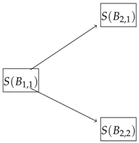 that is
for which the constrains in all one-sided inequalities can be written as
and having the objective function and constrains in matrix form we have
Now we write the dual to this linear programming problem which is
or equivalently

If we let, as an example, , , and , then by solving Equation (27) using linear programming with complementary slackness conditions (we used MATLAB for our purpose) we have (which is the solution to the dual problem and indicates the portfolio strategy one needs to choose in the case of existence of any arbitrage opportunity) and .
Similarly by solving the dual problem for the other part of the diagram
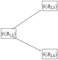 that is
and if we let and also let and , then the solution is and .

Now for the last part consider the following picture and its corresponding linear programming in dual form
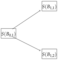

with
for which when (here we simply assumed that ), the corresponding solution becomes and . For any bid price offered at time larger than , there is an arbitrage and the trading strategy is as following:
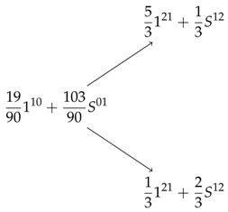 buy units of and units of and at time in either case we are able cover the asked price of at time . In fact in the case of possibility, we buy units of and units of , and in the case of possibility, we buy units of and units of , and in either case will be covered to deliver and the difference will be an arbitrage.

As we noted in the last diagram, at least of the risk-free bond is needed to be bought at time . Now we consider a trading strategy which purchases of the bond bought at time . Therefore the trading strategy can be replaced by
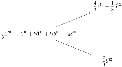 where are the solutions to the new linear programming problem below
and

Solution to the linear programming above is so that the largest ask price for in this case becomes
and as we see, this upper bound is smaller and much more accurate than the upper bound which we found above without using the bond.
Now consider the cash flow and let to be the portion of that we carry in the trading strategy at time . We would like to find the highest ask-price at time for this cash flow. Therefore we consider the following maximization problem and unlike the example above, we try to solve this problem in one step
and by the definition of expectation and letting we have
where
As we can see, the above linear programming is a ten variable linear programming with one parameter and this is only for a binary priced market where at each time there are only two possibilities for the stock and cash flow price. We are only considering one risky asset.
4.4. Complexity of Multi-Period Model
Consider a 2-period model and let be the number of variables in the linear programming associated with this model and be the number of parameters associated with 2-period bonds in this model. We already know that and . We can see that adding a single 1-period bond into the model, adds 2 variables and one parameter to the linear programming problem.
On the other hand a 2-period model is equivalent to a composition of a 1-period model followed by two 1-period models as illustrated in following diagram
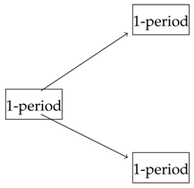

Since a 2-period model is the composition of a 1-period followed by two 1-period models, then = + 2 + 2-period bond =+2+= which coincides with what we found before. This is the case for a over simplified case, binary model with a two states at each time.
Now consider a T-period model and let be the number of variables in the linear programming associated with this model and be the number of parameters associated with multi-period bonds in this model. A T-period model is equivalent to a composition of a 1-period model followed by two -period models as illustrated in following diagram
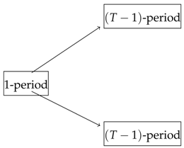

For example, a 3-period model is the composition of a 1-period followed by two 2-period models, so that
= + 2 + 2-period bond + 3-period bond
=+2++=
Now for a T-period model we have
= + 2 + 2-period bond + 3-period bond +⋯+ T-period bond =+2 + + + ⋯ + =
or
=
As it can be seen, when the periods of the model increases, the number of variables and parameters increase at an exponential rate. Considering the fact that this calculation was only done for the simplest case of a model (binary prices and one risky asset) we notice that for a T-period model, the parametrized linear programming with parameters and variables make the problem very complicated to solve.
Lemma 1.
For a T-period model with as the number of variables in the linear programming associated with the model and as the number of parameters associated with multi-period bonds, we have
As a result of the reason explained above, we suggest solving the problem one step at a time, which means (similar to the 2-period linear programming problem that we solved) starting form the end and solving multiple 1-period problems on each step and continuing this process backward until we reach the initial time on the problem.
4.5. Estimate of Multi-Period Bounds (Breaking into One Periods)
Consider the following portfolio of zero-cost cash flows
where
also and . In fact we have the following trading diagram corresponding to the above portfolio at time and
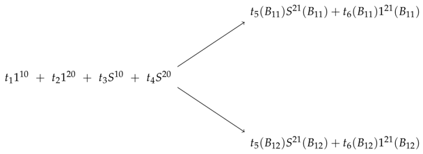

Since we are assuming to deliver at , indeed we have to solve the linear programing problem
We can define the corresponding Lagrangian as
where and are the random variable Lagrange multipliers. Therefore our minimization problem can be stated as
where
Now by Linearity Constraint Qualification the problem is feasible so that by Lagrangian strong duality we have
hence can be written as
We can see that the corresponding maximization problem to the Lagrangian above is
Unsurprisingly, we observe that are the pricing factors in the expectation form. In fact, as we defined before, if we let
then the linear programming in Equation (43) becomes
which, as we can see, is the primal maximization problem (the dual of the dual in this case) corresponding to our initial portfolio. We can also observe that the problem in Equation (45) is indeed the expectation form of a super-hedging problem as
Solving the linear programming problem in Equation (45) we have the following solutions
| 1.3327 | 0.1371 | ||
| 0.5256 | 0.4847 | ||
| 0.2725 | 1.5377 | ||
| 0.0969 | 0.6964 |
with a super-hedging value of
As we notice, there is slightly small decrease on the value of upper bound for the asked price comparing with the case where we calculated this upper bound one step at a time. This is completely justified because the minimization above has more constraints since we are using the two-period bond and asset to formulate our problem. As we stated before, for multi-period cases (that requires us to solve linear models with multiple variables and parameters with a very small adjustments) we will find the upper-bound and lower-bound by solving linear programming problems one at a time.
4.6. The General 2-Period Model
In this section we use the results from the examples in this section to summarize the two different cases on a 2-period model. First case is when one can use all possibilities of bonds and assets (both 1-period and 2-periods).
Theorem 5.
Let , , an acceptable cash flow and consider the following linear programing problem
Then is a super-hedging bound and the solution to dual problem is a portfolio by which one is able to construct an arbitrage opportunity if the market bid price of c exceeds .
Proof.
In Appendix A. □
In this version of the problem one is able to take advantage of the both 2-period bond and assets, however as we saw before there is some complexity in solving and finding the right strategy to construct the portfolio, where as the number of assets and their price possibilities increase, the complexity of finding the right portfolio strategy increases exponentially.
On the other hand, we can find a super-hedge value for a 2-period linear programming problem by solving two 1-period problems successively, in which case we have the following theorem.
Theorem 6.
Let be an acceptable cash flow and suppose
is a super-hedging bound for paid at time (the largest ask price for under no-arbitrage assumption). Now consider the following linear programming problem
then the solution to linear programming problems in Equations (48) and (49) and their duals gives us a trading strategy by which we can take advantage if any arbitrage opportunity is available.
Proof.
In Appendix A. □
As we saw above, we can find a super-hedging bound by two different approaches and because of that there is a slight difference in the values of on these two approaches. The following theorem summarizes our above discussion on an upper bound for the difference between two values.
Theorem 7.
Let and be the two super-hedging values found in Theorem (5) and Theorem (6) respectively. Then
- (1)
- (2)
Proof.
In Appendix A. □
Remark 4.
The upper bound we found above, is an over estimate, but it is small relative to the portfolio price.
5. Multi-Period Case Theorem
The discussion in Section 4 showed that deriving the most accurate super- and sub-hedging bounds is too complex to be practical. An iterative process dealing with one period (bonds and assets) at a time provides a good compromise between accuracy and tractability.
Theorem 8.
Let and consider the following linear programming problem
Then is a super-hedging bound and the solution to dual problem is a trading strategy by which one is able to construct an arbitrage opportunity if the market bid price of c exceeds .
Proof.
In Appendix A. □
Remark 5.
Even though the value of we find in the Theorem above may not be the lowest super-hedging value for the ask price of the cash flow c, it is still a close estimate, as we discussed in Theorem 7 and an upper bound for the exact super-hedging value .
6. Conclusions
We used convex duality in a multi-period conic finance (two-price economy) to extend the refined version of FTAP. This helped us to provide a framework to drive non-arbitrage lower and upper price bounds and corresponding trading strategies which one can take advantage of when a preferable bid (ask) price exists. We also analyzed the computation complexity of implementation in two settings:
- (a)
- using only one-period bonds,
- (b)
- involving all available bonds.
and we showed that involving all available bonds makes the problem unrealistically complex. We provided estimates on the error between the prices for one period and all bonds, which we saw that it is small. Therefore we recommended method dealing only with one-period bonds in practice, where the problems becomes pricing one period at a time. Finding a better approximation for the price bounds and shrinking the non-arbitrage region and lowering the computation complexity are two problems that one could consider for further exploration.
Author Contributions
M.V. and Q.J.Z. contributed equally to this research. All authors have read and agreed to the published version of the manuscript.
Funding
This research received no external funding.
Conflicts of Interest
The authors declare no conflict of interest.
Appendix A. Proofs
Proof of Theorem 1.
(⇒) If there is some arbitrage , then, for any , since is a convex cone, . When , we know that
therefore .
(⇐) If , there exists a sequence for which
Since u is continuous and increasing, we have . For , let and suppose
then . By the condition on the domain of utility function , we need to have or . Dividing both sides by we have
so that for . This means that is an arbitrage. □
Proof of Theorem 3.
The sufficient condition of the theorem is clear. For the necessary part, consider the primal problem above. We know that the initial endowment , also and so that and the Constraint Qualification is satisfied, where is the support of f on which f is continuous. Since Constraint Qualification holds, by applying the Strong Duality for the primal p and dual problem
we have . Therefore,
If are the solutions to the primal and dual problems, then . We need to have . Let be the conditional expectation with respect to . Since for any set , we have
which implies or
Using the definition above and by letting as the pricing factor, Equation (A1) can be written as
For any (here is the characteristic function on set O), so that
□
Proof of Theorem 4.
Let and
subject to
Here we will be formulating the dual problem. To that purpose define the Lagrangian as
where
and all for are non-negative constants.
First, it can be seen that
Therefore, we can write
On the other hand, for non-negative constants
we can recognize
Now, under no-arbitrage assumption, the primal linear programming problem has a finite value, hence the Constraint Qualification is satisfied (under no-arbitrage assumption the primal problem has a finite value, therefore feasible) so that both primal and dual problems has solutions, therefore by strong duality we have
If we consider to be the premium (received at time ) for delivering at time , then simply the problem becomes to build a zero cost portfolio so that the overall transaction, is an arbitrage. Thus, one should have,
The last equation then, in terms of the dual linear programming problem can be written as
Under no-arbitrage assumption we know this linear programming problem has a finite value and a solution exists. Let be the solution of this dual problem. Since the feasibility condition is satisfied, there exists (solution to the primal problem) such that
Now suppose,
then there are non-negative constants and by which we can construct a zero cost trading strategy such that
□
Proof of Theorem 5.
As we saw in Section 4.5 the dual problem to linear programming in Equation (47) is
where
is the zero-cost cash flow (portfolio) as our trading strategy and to be more precise
is the cost of building such portfolio to be paid at time . In addition,
where as indicated, has two parts, one is the pay-off and the other is the adjustment at time . is entirely the pay-off where
A solution to linear programming problem (A5) is a set of non-negative coefficients that determine the trading strategy to super-hedge. Specifically tell us about the number of shares of 2-period bonds and traded at . □
Proof of Theorem 6.
The dual problem of Equation (48) is given by
where
and the non-negative -measurable random variables determine the trading strategy form to .
Similarly the dual problem of Equation (49) is
where
is a zero-cost cash flow and the non-negative -measurable random variables determine the trading strategy form to . We notice that
is the cost of this portfolio paid at . □
Proof of Theorem 7.
- (1)
- (2)
- We start the argument by looking in a few easier and more concrete cases.
- (a)
- Consider the case where a super-hedging bound of is found by only zero-coupon bonds (a 2-period bond or two 1-period bonds ). Then the price difference would be
- (b)
- If we assume that there is only one asset with two options (a 2-period or two 1-period ) then the difference in the hedging-price values is
- (c)
- Now if we use both bond and asset then we have an upper bound for the difference as
- (d)
- Therefore for a super-hedging with both bonds and finite number (M) of assets we have□
Proof of Theorem 8.
As a result of what was discussed in Lemma 1 (the complexity in solving the dual linear programming problem) we solve and find the trading strategy starting at T− 1 going backward and one step at a time. So first let
We formulate the dual problem by using the Lagrangian. First let
be the Lagrange multiplier of our linear programing problem. So we can write the Lagrangian as
Now we can observe that
So that, by strong linear programming duality we have
On the other hand, the Lagrangian can be rewritten as
Now for consider the zero-cost portfolio of cash flow
so that
and
Since the term is an measurable random variable and independent of , then we see that Equation (A25) can be written as
Now let
Let for all . Then Equation (A24) becomes
If is a solution to the minimization problem in Equation (A32), then it determines the trading strategy from time to time T while is the highest price for (with no-arbitrage) paid at time . Therefore we set up a linear programming problem that determines a super-hedging value of both and paid at time , as following
Similar to what we did above on establishing and solving the dual problem, suppose is the solution to dual linear programming problem of Equation (A33), then it determines the trading strategy form time to . Continuing this backward process and one step at a time, we will have a sequence of pairs, super-hedges and non-negative random variable coefficients
where
and the first term in Equation (A34) is the super-hedging value and the corresponding trading strategy coefficients determined at time . Now we set-up our last linear programming problem where we find the super-hedging bound for . Let
with the corresponding Lagrangian
so that
If is a solution to the minimization problem in Equation (A39) then, in fact, it determines the trading strategy from time t to time and along with the other non-negative random variable coefficients we have created a trading strategy corresponding to
with the super-hedging bound by which one can create an arbitrage opportunity if any higher price in the market is available. □
References
- Artzner, Philippe, Freddy Delbaen, Jean-Marc Eber, and David Heath. 1999. Coherent measures of risk. Mathematical Finance 9: 203–28. [Google Scholar] [CrossRef]
- Bion-Nadal, Jocelyne. 2009. Bid-ask dynamic pricing in financial markets with transaction costs and liquidity risk. Journal of Mathematical Economics 45: 738–50. [Google Scholar] [CrossRef]
- Carr, Peter, Helyette Geman, and Dilip B. Madan. 2001. Pricing and Hedging in Incomplete Markets. Journal of Financial Economics 62: 131–67. [Google Scholar] [CrossRef]
- Carr, Peter, and Qiji Jim Zhu. 2018. Convex Duality and Financial Mathematics. Berlin and Heidelberg: Springer. [Google Scholar]
- Cherny, Alexander, and Dilip B. Madan. 2009. New Measures for Performance Evaluation. Review of Financial Studies 22: 2571–606. [Google Scholar] [CrossRef]
- Cherny, Alexander, and Dilip B. Madan. 2010. Markets as a Counterparty: An Introduction to Conic Finance. International Journal of Theoretical and Applied Finance 13: 1149–77. [Google Scholar]
- Constantinides, George M. 1986. Capital Market Equilibrium with Transaction Costs. Journal of Political Economy 94: 842–62. [Google Scholar] [CrossRef]
- Copeland, Thomas E., and Dan Galai. 1983. Information Effects on the Bid-Ask Spread. Journal of Finance 38: 1457–69. [Google Scholar] [CrossRef]
- Delbaen, Freddy, and Walter Schachermayer. 1994. A General Version of the Fundamental Theorem of Asset Pricing. In The Mathematics of Arbitrage. Berlin and Heidelberg: Springer, pp. 149–205. [Google Scholar]
- Eberlein, Ernst, Thomas Gehrig, and Dilip B. Madan. 2009. Accounting to Acceptability: With Applications to the Pricing of One’s Own Credit Risk. Robert H. Smith School Research Paper No. RHS 06-113. SSRN Electronic Journal. [Google Scholar] [CrossRef]
- Eberlein, Ernst, and Dilip B. Madan. 2009. Hedge fund performance: Sources and measures. International Journal of Theoretical and Applied Finance 12: 267–82. [Google Scholar] [CrossRef]
- Eberlein, Ernst, and Dilip B. Madan. 2012. Unbounded liabilities, capital reserve requirements and the tax payer put option. Quantitative Finance 12: 709–24. [Google Scholar] [CrossRef]
- Eberlein, Ernst, Dilip B. Madan, and Wim Schoutens. 2011. Modeling risk weighted assets and the risk sensitivity of related capital requirements. Journal of Risk, 16. [Google Scholar] [CrossRef]
- Guasoni, Paolo, Emmanuel Lepinette, and Miklós Rasonyi. 2011. The Fundamental Theorem of Asset Pricing Under Transaction Costs. Boston U. School of Management Research Paper, No. 2011-7. Mathematical Finance 14: 19–48. [Google Scholar]
- Harrison, J. Michael, and David Kreps. 1979. Martingales and arbitrage in multi-period securities markets. Journal of Economic Theory 20: 381–408. [Google Scholar] [CrossRef]
- Harrison, J. Michael, and Stanley R. Pliska. 1981. Martingales and stochastic integrals in the theory of continuous trading. Stochastic Processes and Their Applications 11: 215–60. [Google Scholar] [CrossRef]
- Jacka, Saul D. 1992. A martingale representation, result and an application to incomplete financial markets. Mathematical Finance 2: 239–50. [Google Scholar] [CrossRef]
- Jouini, Elyès, and Hédi Kallal. 1995. Martingales and Arbitrage in Securities Markets with Transaction Costs. Journal of Economic Theory 66: 178–97. [Google Scholar] [CrossRef]
- Madan, Dilip B, and Wim Schoutens. 2011. Conic coconuts: The pricing of contingent capital notes using conic finance. Mathematics and Financial Economics 4: 87–106. [Google Scholar] [CrossRef]
- Madan, Dilip B., and Wim Schoutens. 2012. Structured products equilibria in conic two-price markets. Mathematics and Financial Economics March 6: 37–57. [Google Scholar] [CrossRef]
- Madan, Dilip B. 2012. A two price theory of financial equilibrium with risk management implications. Annals of Finance 8: 489–505. [Google Scholar] [CrossRef]
- Madan, Dilip B. 2015. Asset pricing theory for two price economies. Annals of Finance 11: 1–35. [Google Scholar] [CrossRef]
- Rogers, Leonard Christopher Gordon. 1994. Equivalent martingale measures and no-arbitrage. Stochastics and Stochastics Reports 51: 41–49. [Google Scholar] [CrossRef]
© 2020 by the authors. Licensee MDPI, Basel, Switzerland. This article is an open access article distributed under the terms and conditions of the Creative Commons Attribution (CC BY) license (http://creativecommons.org/licenses/by/4.0/).