Copula-Based Assessment of Co-Movement and Tail Dependence Structure Among Major Trading Foreign Currencies in Ghana

Abstract

This paper examines the joint movement and tail dependence structure between the pair of foreign exchange rates (EUR, USD and GBP) against the GHS, using daily exchange rates data expressed in GHS per unit of foreign currencies (EUR, USD and GBP) between the time range of 24 February 2009 and 19 December 2019. We use different sets of both static (time-invariant) and time-varying copulas with different levels of dependence and tail dependence measures, and the study results reveal positive dependence between all exchange rates pairs, though the dependencies for EUR-USD and GBP-USD pairs are not as strong as the EUR-GBP pair. The findings also reveal symmetric tail dependence, and dependence evolves over time. Notwithstanding this, the asymmetric tail dependence copulas provide evidence of upper tail dependence. We compare the copula results to DCC(1,1)-GARCH(1,1) model result and find the copula to be more sensitive to extreme co-movement between the currency pairs. The afore-mentioned findings, therefore, offer forex market players the opportunity to relax in hoarding a particular foreign currency in anticipation of domestic currency depreciation.

1. Introduction

Major financial institutions and investors are concerned about extreme complexity and high volatility of financial markets, most especially the global currency markets which are known to dominate other markets such as stock and bond markets. This is attributed to the internationalization of modern business, the continuing growth in world trade relative to national economies, the trend towards economic integration and the rapid pace of change in money transfer technology, which all account for the increased importance of exchange rates (Copeland 2008). Foreign exchange markets are highly interlinked with other financial markets such that its fluctuations have a pervasive effect on market participants including governments, central banks, big banks, multinational corporations, currency speculators and individuals. The dynamics of exchange rates, especially in a floating exchange rates regime, have practical implications for international traders, investors, analyst and policymakers. Because movement in exchange rates affect the expected profitability and risk of financial assets, investors in international financial markets need a reliable estimate for portfolio optimization and diversification. From the perspective of monetary policy authorities and economic policymakers, understanding the dynamics of exchange rates provide an avenue for economic policy assessment and international economic policy coordination.

The measurement of dependence of international financial markets during a period of extreme fluctuations has received considerable attention in the extant literature. One of the interesting features of exchange rates has been the question of whether volatilities in financial markets are interrelated and whether such linkages are constant or vary over time. Studies that have focused on co-movement and interdependence of returns of financial assets show that conditional covariances and conditional correlations between returns of assets vary largely over time (see Bollerslev et al. 1988; Engle 2002) and co-movement in times of financial distress are significantly higher than during tranquil times (see Loaiza-Maya et al. 2015a, 2015b). The extreme co-movement between returns of financial assets during a period of financial distress has been described in financial literature as contagion. In as much as studies on co-movement among returns of financial assets have focused extensively on the stock market in the literature (see Karolyi and Stulz 1996; Forbes and Rigobon 2002; Brooks and Del Negro 2004; Boako and Alagidede 2017b), exchange rates co-movement have not been completely left out (see Engle et al. 1988; Pérez-Rodríguez 2006; Patton 2006; Dias and Embrechts 2010; Antonakakis 2012; Tamakoshi and Hamori 2014; Beirne and Gieck 2014).

Though currency markets co-movement capture how shocks in a specific market may transcend to other currency markets, currency movements are not only influenced by country-specific and idiosyncratic factors such as economic fundamentals and monetary policy direction but also by other external drivers. Therefore, measuring co-movements and tail dependence structures and ascertaining the volatility spillover associated with exchange rates and their evolution over time is very essential in risk management, diversification and pricing.

Interestingly, studies on the co-movement of exchange rates concentrate on inter-country/regional analysis, although the number of studies is small (Junior et al. 2019). However, to control for country-specific factors and idiosyncratic factors, intra-country studies present different dimensions to exchange rates interdependency among major trading currencies in an economy. In most developing countries, multiple currencies are utilized in foreign and local transactions; therefore, proper understanding of their interactions is necessary for monetary policy and currency risk management.

Like most currencies in developing countries, Ghana cedi continuously depreciates against its major trading currencies near major festive period (e.g., Christmas, Ramadan, etc.) due to pressure from importers to meet the demands of the festivities and repatriation of earning by multinational companies at the end of the financial year. This confronting issue impacts the economic management of these economies. For example, the Ghana cedi has depreciated against the US dollar by about 99.98% over the last three decades.

In times of extreme market conditions, currency markets tend to co-move more than in tranquil or normal times. The market participants need to know which foreign currency dictates the co-movement and the interdependences. Usually, in the case of Ghana, participants in the currency markets focus their attention on the US dollar by hoarding it in anticipation of depreciation of the cedi. But should the concentration only be on the US dollar during periods of extreme depreciation of the cedi against other foreign currencies? It is important to note that severe depreciation of the cedi against the US dollar is likely to occur jointly with depreciation against other foreign currencies more than the appreciation of the cedi against the US dollar and other foreign currencies. This leads to the fact that the tail dependence structure between the exchange rate markets is asymmetric and the use of Pearson correlation, which thrives on using a symmetric multivariate normal distribution or student t-distribution, fails to capture such asymmetric tail dependence of the markets (see Patton 2006; Garcia and Tsafack 2011).

This study employs a static and time-varying copula to capturing the asymmetric tail dependence between the major trading currencies (US dollar (USD), euro (EUR) and British pound (GBP)). The choice of copula model for the study is appropriate because studies have shown that distribution of return of financial assets exhibits properties such as long memory, heteroscedasticity and fat tail. Also, exchange rates tend to jointly depreciate against one currency more than appreciating together, making the distribution of returns asymmetric. The copular function introduced by Sklar (1959) gives us the flexibility to combine univariate distributions to obtain a joint distribution with a particular dependence structure. Another advantage of using the copula function is its ability to model dependence in extreme market conditions and to extract both the degree and structure of the dependence. Besides, as alluded by Patton (2012) that the flexibility copula models provide in modeling multivariate distributions is by fitting models for the marginal distributions separately from the copula that connects the marginals to form the joint distribution. What makes copulas so unique from other linear correlation measures of dependence is the fact that copula functions are invariant to strictly increase non-linear data transforms (Embrechts et al. 2002).

Our study is the first to examine the co-movement and tail dependence structure of the three major exchange rates (GHS/USD, GHS/EUR and GHS/GBP). It implements a copula-based approach in quantifying the degree and evolution of co-movement and tail dependence structure among exchange rates on Ghana’s currency markets. The study differs from the most recent study conducted by Junior et al. (2019) in a methodological approach which used wavelet coherence analysis to explore the interdependence of major exchange rates in Ghana. The wavelet coherence is unable to reveal the existence of tail dependence structure among the exchange rates.

The results of the study show positive dependence between all exchange rates pairs, though the dependencies for EUR-USD and GBP-USD pairs are not as strong as for the EUR-GBP pair. The results further reveal symmetric tail dependence between the exchange rates pairs, and dependence evolves. Notwithstanding, the asymmetric tail dependence copulas provide evidence of upper tail dependence, implying that the foreign currencies are more likely to jointly appreciate more than depreciating against the domestic currency (GHS). This means that the fall in the value of GHS is more profound than appreciating. Furthermore, the copula model results prove to be more sensitive to extreme co-movement between the exchange rate pairs than the DCC-GARCH model. The remaining sections of this study are structured as follows: Section 2 presents brief literature on exchange rates co-movements and dependence structure, Section 3 shows methodology and data description while in Section 4 and Section 5, we present our study results and conclusion, respectively.

2. Literature Review

Co-movement of financial markets have received considerable attention in the literature and establishing the nature of dependence especially in currency pairs is very significant. The vast number of papers addressing co-movements and dependencies of financial markets have delved more into stock markets, while less attention is focused on exchange rate markets. Meanwhile, a handful of studies have focused on co-movements and dependencies between exchange rates and other forms of financial assets such as stocks and commodities (see Tai 2007; Büttner and Hayo 2010; Wu et al. 2012; Wang et al. 2013; Pal et al. 2014; Chkili and Nguyen 2014; Apostolakis and Papadopoulos 2015; Dua and Tuteja 2016). Earlier studies that investigated exchange rates interdependencies used linear correlation models such as the vector autocorrelation models, cointegration approach and the generalized autoregressive conditional heteroskedasticity models (GARCH).

Engle et al. (1988) used the GARCH model to predict whether news in the New York market could cause volatility in the Tokyo market after many hours later by examining the yen/dollar exchange rate. Their study reveals that exchange rates react not only to shocks from macroeconomic fundamentals in the domestic market but also to the transmission of spillovers from other markets. After the pioneering paper of Engle et al. (1988), Pérez-Rodríguez (2006) and Tamakoshi and Hamori (2014) used GARCH models to examine exchange rate returns interdependence. Also, the dynamic correlation GARCH-type models proposed by Engle (2002) were extended by Cappiello et al. (2006) to capture asymmetric dependence between returns of financial assets have extensively been used to investigate co-movement and volatility spillovers between major exchange rates (see Antonakakis 2012; Dimitriou and Kenourgios 2013; Tamakoshi and Hamori 2014).

Aside from the dominant use of GARCH models to explore exchange rates linkages and interdependencies, other approaches have been well utilized in the literature. Wu (2007) used an empirical-mode decomposition approach to investigate the correlation of the Deutsche Mark and Japanese rates against the US dollar from 1 February 1986 to 31 December 1996. The study reveals that correlation between the two currencies was higher in the early part of the study period than in the later period. To establish that the distribution of correlation coefficients concerning relative return in currency prices is dependent on time, Jiang et al. (2007) employed the random matrix theory to explore the level of correlation among 74 global currencies. Wang and Xie (2013) implemented the detrended cross-correlation method and found significant cross-correlation between the Chinese renminbi and other four currencies including the US dollar, Euro, Japanese yen and the Korean won. Moreover, Heni and Mohamed (2011) carried out an empirical analysis on daily Tunisian exchange rates co-movements concerning the US dollar, the Euro and Japanese yen using discrete wavelet transform and concluded that exchange rate series exhibit generalized long memory. Also, Kumar et al. (2017) used multiple wavelet correlation and cross-correlation analysis to study the co-movement in daily returns of the US dollar, Euro, British pound and Japanese yen futures contracts on India’s National Stock Exchange between 1 February 2010 and 26 August 2014 inclusive. They concluded that the currency futures markets are almost perfectly integrated in the long run with some inconsistencies that fade away within 3 to 6 months.

However, the afore-mentioned approaches failed to ascertain the asymmetric dependencies between exchange rates, as studies have shown that the degree to which exchange rates jointly appreciate and depreciate differ (see Patton 2006). Therefore, copula models have been employed extensively in the literature to study co-movement and tail dependence structure between returns of financial assets. Even though the use of copula models has been a common approach recently in assessing co-movements and tail dependence structure, a plethora of the studies have focused on stock markets (see He 2003; Hu 2006; Yang and Hamori 2013; Yang et al. 2015; Boako and Alagidede 2017a). Notwithstanding this, a handful of studies have used copula models to examine exchange rates co-movements after the pioneering work of Patton (2006) who discovered after modeling asymmetry dependence between the Deutschemark and the yen against the US dollar, that two exchange rates jointly move against the US dollar when they are depreciating more than when they are appreciating.

In addition, Dias et al. (2004) examined dynamic dependence between the Deutschemark and the Yen using copulas at high frequencies (two, four, eight, twelve-hour and one day period) and found out that the dependence structure varied overtime at all frequencies. Benediktsdóttir and Scotti (2009) employed conditional copula approach to study the dependence structure of several exchange rates against the dollar and investigated whether dependence structures were affected by business cycles or interest rate differentials. Their results show that dependencies are time-varying, that foreign and US recessions affect the joint dependence structure and that currencies with higher interest rate differentials tend to move less closely together, even at extreme events. Albulescu et al. (2018) investigated the bivariate dependence structure between four international exchange rates (EUR, GBP, CAD, JPY) against the US dollar using daily data from 1999–2014. Their study reveals positive dependence between all exchange rates, except JPY-pairs of exchange rates and finds evidence of symmetric tail dependence and dependence is time-varying. Our study departs from the latter by considering exchange rates of USD, EUR and GBP against Ghana Cedi (GHS), which experienced intense pressure from international activities. Our study is closer to Junior et al. (2019), who employed wavelet coherence analysis to explore the co-movement amongst the returns of four major currencies in Ghana (dollar, euro, pound and yen) from May 1999 to February 2018. Their empirical findings showed that the currencies are closely linked or interconnected and the lead-lag relationships between the returns of the exchange rates established that volatilities in the euro and yen significantly affect movements in the other currencies. The current study differs in terms of methodology.

3. Methodology

The basic approach in capturing dependence between two random variables has been the use of the Pearson linear correlation coefficient and non-parametric measures such as Kendall’s tau and Spearman’s rho correlation. Though these measures try to establish a link between two random variables, they do not provide any information about the dependence structure or tail dependence between the variables. Since the financial time series generally exhibit some characteristics such as long memory, fat-tail and heteroskedasticity, the use of copula models introduced by Sklar (1959) are capable of identifying not only the linear association between the return series but importantly, the tail dependence of the joint distribution between returns of the series. Copula function decomposes n-dimensional joint distribution function into its marginal distributions and a copula that completely describes the dependence between the n variables (Patton 2006). Therefore, using Sklar’s theorem, the dependence structure between variables of interest can be modeled by first specifying the marginal distributions of the variable of interest and then specifying a copula which will connect the marginal distributions to form joint distribution of the variables of interest, if the exchange rates return.

3.1. Specifying the Marginal Models

Models for each marginal distribution are specified first before a bivariate copula model is fitted. Because financial time series are characterized by some features such fat-tails, long-memory and heteroskedasticity, it is very necessary to have these characteristics captured using an autoregressive moving average (ARMA) and generalized autoregressive conditional heteroskedasticity (GARCH) models. Thus the ARMA(k,m)-t-GARCH(p,q) models for the logarithm exchange rate return series $Y_{it}$ is described as follows:

$$Y_t={\varnothing }_0+{\displaystyle \sum }_{i=1}^k{\varnothing }_i{Y}_{t-i}+{\displaystyle \sum }_{j=0}^m{\theta }_j{\epsilon }_{t-j}+{\epsilon }_t$$

(1)

$${\epsilon }_t={\sigma }_t{z}_t, z_t~i.i.d.t_v$$

(2)

$${\sigma }_t^2={\alpha }_0+{\sum }_{h=1}^p{\alpha }_h{\epsilon }_{t-h}^2+{\sum }_{l=1}^q{\beta }_l{\sigma }_{t-l}^2, .$$

(3)

Equations (1)–(3) represent respectively, the mean, the error and variance equations and $Y_t$ is the logarithm exchange rate return at time t, ${\epsilon }_t$ is the real-valued discrete-time stochastic process of exchange rate return at time t, $z_t$ is an i.i.d unobserved random variable with zero mean and constant variance, $v$ is the degree of freedom for the student-$t$ distribution and ${\sigma }_t^2$ is the conditional variance of ${\epsilon }_t$. k, m, p and q are non-negative integers representing the order of AR, MA, ARCH and GARCH terms, respectively; ${\varnothing }_0 and {\alpha }_0$ are constants, ${\varnothing }_i$ and ${\theta }_j$ are the respective AR and MA parameters of the mean equation while ${\alpha }_h and {\beta }_l$ are respectively the parameters of the ARCH and GARCH components of the variance equation, where ${\alpha }_j+{\beta }_j<1$.

3.2. Specifying the Copula Models

According to Sklar (1959), multivariate distribution can be decomposed into univariate marginal distributions and a copular that fully captures the dependence between the marginals. Generally, given n-variate cumulative distribution function and its univariate marginals respectively as $F_{X_1,\dots ,X_n}\left(x_1,\dots ,x_n\right)$ and $F_{X_i}\left(x_i\right), i=1,\dots .,n, x_i\in \left(-\infty ,\infty \right)$, then there exists a copula function C that maps ${\left[0,1\right]}^n$ into $\left[0,1\right]$ such that

$$F_{X_1,\dots ,X_n}\left(x_1,\dots ,x_n\right)=C\left[F_{X_1}\left(x_1\right),\dots ,F_{X_n}\left(x_n\right)\right].$$

(4)

The above expression shows copula formulation for n number of assets but specifically for establishing dependence and co-movement between two assets at a time, a bivariate joint distribution model is formulated. For example, given two random variables $X_1$ and $X_2$ with marginal distributions $F_1\left(x_1\right)$ and $F_2\left(x_2\right)$, we can define their joint cumulative distribution function $F\left(x_1,x_2\right)$ as:

$$F_{X_1{X}_2}\left(x_1,x_2\right)=C\left[F_{X_1}\left(x_1\right),F_{X_2}\left(x_2\right)\right].$$

(5)

If $F_{x1}$ and $F_{x2}$ are continuous, then $C$ is unique and is uniquely defined on $Ran{F}_{x1}\times Ran{F}_{x2}$. Separating the joint distribution into marginal parts and the dependence structure (copula) without losing any information, is one of the important properties attributed to copula functions. Again, the tail dependence between the two random variables $X_1$ and $X_2$ is invariant under the strictly increasing transformation of $X_1$ and $X_2$. The lower (left) tail ${\tau }_l$ and upper (right) tail ${\tau }_u$ dependence between $X_1$ and $X_2$ can be defined following previous studies as

$${\tau }_l=li{m}_{u\to 0}P\left(F_{X_1}\left(x_1\right)\le u|F_{X_2}\left(x_2\right)\le u\right)=li{m}_{u\to 0}\frac{C\left(u,u\right)}{u}$$

(6)

$${\tau }_U=li{m}_{u\to 1}P\left(F_{X_1}\left(x_1\right)\ge u|F_{X_2}\left(x_2\right)\ge u\right)=li{m}_{u\to 1}\frac{1-2u+C\left(u,u\right)}{1-u}$$

(7)

where${\tau }_l$ and${\tau }_U ϵ \left[0,1\right]$. If ${\tau }_l>0$ and ${\tau }_u>0$, $X_1$ and $X_2$ tend to be lower (left) or upper (right) tail dependent. The tail dependence which measures the probability that both variables are in their lower and upper joint tails captures the behavior of the random variables during extreme events. Thus, for this study, an extremely small (large) value for one exchange rate jointly moves with an extremely small (large) value for another exchange rate when ${\tau }_l\ne {\tau }_U$ and ${\tau }_l>0({\tau }_U>0)$.

To capture the tail dependence of a different pattern, time-invariant and time-varying copulas of different specifications and characteristics so far as tail dependence measurement is concerned are considered in this study. These include Gaussian copula, Student-t copula, Gumbel copula, rotated Gumbel copula, Clayton and rotated Clayton copulas. The Gaussian copula which is unable to capture tail dependence is chosen to assess co-movement based on the traditional linear correlation measure which allows for equal degrees of positive and negative dependence. The Student-t copula captures the strength of symmetric extreme dependence and represents a generalization of the Gaussian copula with non-zero dependence in the tails. The family of Archimedean copulas such as Gumbel and rotated Gumbel copulas, Clayton and rotated Clayton copulas show asymmetric tail dependence. If we assume that co-movements increase more in financial turbulence periods, then Clayton or rotated Gumbel copulas is recommended. On the other hand, if we assume that co-movements increase more in periods of economic boom, then Gumbel or rotated Clayton copula is recommended. The corresponding copula model specifications and their dependence parameters that measure the strength of this dependence are described briefly below:

• Gaussian copula allows for equal degrees of positive and negative dependence but does not allow for tail dependence, implying that the tail parameters ${\tau }_l={\tau }_U=0$. Therefore, the dependence parameter of Gaussian copula is Pearson’s correlation coefficient (ρ) with a range of values: $-1<\rho <1$. The bivariate Gaussian copula is defined by $C_N\left(u,v|\rho \right)=\mathsf{\Phi }\left({\mathsf{\Phi }}^{-1}\left(u\right),{\mathsf{\Phi }}^{-1}\left(v\right)\right)$, where $\mathsf{\Phi }$ and ${\mathsf{\Phi }}^{-1}$ are respectively the cumulative and inverse cumulative distribution functions of the standard normal distribution.
• Student-t copula allows for symmetric non-zero dependence in the tails and it is the generalization of the Gaussian copula. With the degree of freedom $\eta$ and correlation coefficient $\rho$, the Student-t copula can be defined by $C_{\eta ,\rho }\left(u,v\right)=t_{\eta ,\rho }\left(t_{\eta }{}^{-1}\left(u\right),t_{\eta }{}^{-1}\left(v\right)\right)$, where $t^{-1}$ is the inverse function of the univariate Student’s t distribution.
• Gumbel copula is asymmetric which shows a higher probability of upper tail dependence defined by ${\tau }_U=2-2^{1/\delta }$ and lower tail dependence $({\tau }_L=0)$. Gumbel copula is specified as $C_G\left(u,v|\delta \right)=\exp \left(-\left({\left(lnu\right)}^{\delta }\right)+{\left(-lnv\right)}^{\delta }{)}^{\frac{1}{\delta }}\right)$, where the dependence parameter $\delta \in [1,\infty )$ and does not allow for negative dependence and the case of independence, $\delta =1$.
• The rotated Gumbel copula measures lower (left) tail dependence with the parameter $\delta \in [1,\infty )$ and $\delta =1$ implies independence. Thus, it is appropriate when the variables are highly correlated at low values and does not allow for negative dependence. The lower tail dependence ${\tau }_L$ is then defined as ${\tau }_L=2-2^{1/\delta }$ and the upper tail dependence ${\tau }_U=0$.
• The Clayton copula is asymmetric which exhibit more dependence in the lower (left) tail than the right with parameter $\theta \in \left[1,\infty \right)$ and $\theta =1$, implies independence. The Clayton copula is specified as $C_{Cl}\left(u,v|\theta \right)={\left(u^{-\theta }+v^{-\theta }-1\right)}^{-\frac{1}{\theta }}$. The lower tail dependence probability is defined by ${\tau }_L=2^{-\frac{1}{\theta }}$ and the upper tail dependence probability ${\tau }_U=0$.

Dynamic evolution of the Gaussian and Student-t copulas parameter, ${\rho }_t$ is modeled following Patton’s (2006) approach, as an autoregressive moving average process;

ARMA (1,$q$) specified as:

$${\rho }_t=\wedge \left[{\mathsf{\Psi }}_0+{\mathsf{\Psi }}_1{\rho }_{t-1}+{\psi }_2\frac{1}{q}{\displaystyle \sum }_{j=1}^q{\mathsf{\Phi }}^{-1}\left(u_{t-j}\right).{\mathsf{\Phi }}^{-1}\left(v_{t-j}\right)\right]$$

(8)

where $\wedge \left(x\right)=\frac{1-e^{-x}}{1+e^{-x}}$ is a transformation function that holds the correlation parameter ${\rho }_t$ in the interval $\left(-1,1\right)$ and $u_t$ and $v_t$ are probability integral transformation of the margins. The specification of Equation (8) follows the ARMA $\left(1,q\right)$ process where the AR part captures the persistence in the dependence parameter and the variation effect independence is captured by the average product of the transformed variables ${\mathsf{\Phi }}^{-1}\left(u_{t-j}\right)$ and ${\mathsf{\Phi }}^{-1}\left(v_{t-j}\right)$ over the previous $q$ lags.

The Archimedean copulas (Gumbel, rotated Gumbel, Clayton and rotated Clayton) are estimated using the Generalized Autoregressive Score (GAS) model of Creal et al. (2013). This approach assumes that the copula parameter evolves as a function of its own lagged value and a forcing variable that relate to the scaled score of the copula log-likelihood. The choice of GAS model for modeling time-varying Archimedean copulas is its sensitivity to the off-diagonal observations and observations in the lower and upper tail. The GAS approach uses strictly increasing transformation (logarithm transform) to copula parameters to guarantee that the parameters are constrained to lie in a particular range (e.g., $\rho \in \left(-1,1\right)$). Following Patton (2012), the evolution of the transformed parameter is denoted by:

$$f_t=h\left({\delta }_t\right)\iff {\delta }_t\iff h^{-1}\left(f_t\right)$$

(9)

where

$$f_{t+1}=\omega +\beta f_t+\alpha I_t{}^{-1/2}{s}_t$$

(10)

$$s_t\equiv \frac{\partial }{{\partial }_{\rho }}logc\left(u_t,v_t;{\delta }_t\right)$$

(11)

$$I_t\equiv E_{t-1}\left[s_t{s^{\prime }}_t\right]=I\left({\delta }_t\right).$$

(12)

These expressions show that the future value of the copula parameter depends on a constant, the present value and the score of the copula log-likelihood $I_t{}^{-1/2}{s}_t$.

3.3. Estimation Procedure

The copula parameters are estimated using two-stage maximum likelihood (ML), following the approach of Patton (2006). With the two-stage maximum log-likelihood approach for estimating the parametric copulas, the model that provides the best fit for the individual variables are first estimated, followed by the estimation of the dependence structure of the copula. The log-likelihood function for estimating the parameters is written below as:

$$f\left(\psi \right)={\displaystyle \sum }_{t=1}^T\left[ln{f}_{X_1}\left(x_{1,t};a_{X_1}\right)+ln{f}_{X_2}\left(x_{2,t};a_{X_2}\right)+lnc\left\{\left(F_{X_{1,t}};a_{X_1}\right),F_{X_2}\left(x_{2,t};a_{X_2}\right);\theta \right\}\right]$$

(13)

where $a_{x_1}$ and $a_{x_2}$ are the parameters of the marginal distribution of $X_1$ and $X_2$, $\theta$ is the copula density parameter and $\psi$ is the joint density parameter.

With the two-stage likelihood estimation approach, the parameters of the marginal distributions that provide the best fit for the individual variables are first estimated as:

$$a_{X_1,X_2}=arg\underset{a_{X_1,X_2}}{\max }{\sum }_{t=1}^T{f}_i\left(x_{1,t}{x}_{2,t};a_{X_1,X_2}\right).$$

(14)

The dependence parameter of the copula is estimated in the second stage as:

$$\theta =arg\underset{\theta }{\max }{\sum }_{t=1}^{T}lnc\left({\widehat{u}}_t,{\widehat{v}}_t;\theta \right),$$

(15)

where ${\widehat{u}}_t=F_{X_1}\left(x_{1,t};{\widehat{a}}_{X_1}\right)$ and ${\widehat{v}}_t=F_{X_2}\left(x_{2,t};{\widehat{a}}_{X_2}\right)$.

3.4. Data and Data Description

The data set is composed of daily returns of nominal exchange rates of three major currencies namely the US dollar (USD), the British pound (GBP) and the Euro (EUR) against the Ghana cedi (GHS) obtained from DataStream. The time window spans from the period 24 February 2009, to 19 December 2019. The nominal exchange rates are the prices of a unit each of foreign currency in GHS terms so that if the exchange rate increases (decreases), the GHS is depreciating (appreciating) against the foreign currency. The returns of the nominal exchange rates were obtained by the computation below:

$$r_t=\ln \left(1+R_t\right)=\ln \left(P_t\right)-\ln \left(P_{t-1}\right)$$

(16)

where $r_t$ is the continuously compounded return, $P_t$ and $P_{t-1}$ are the respective current and previous prices.

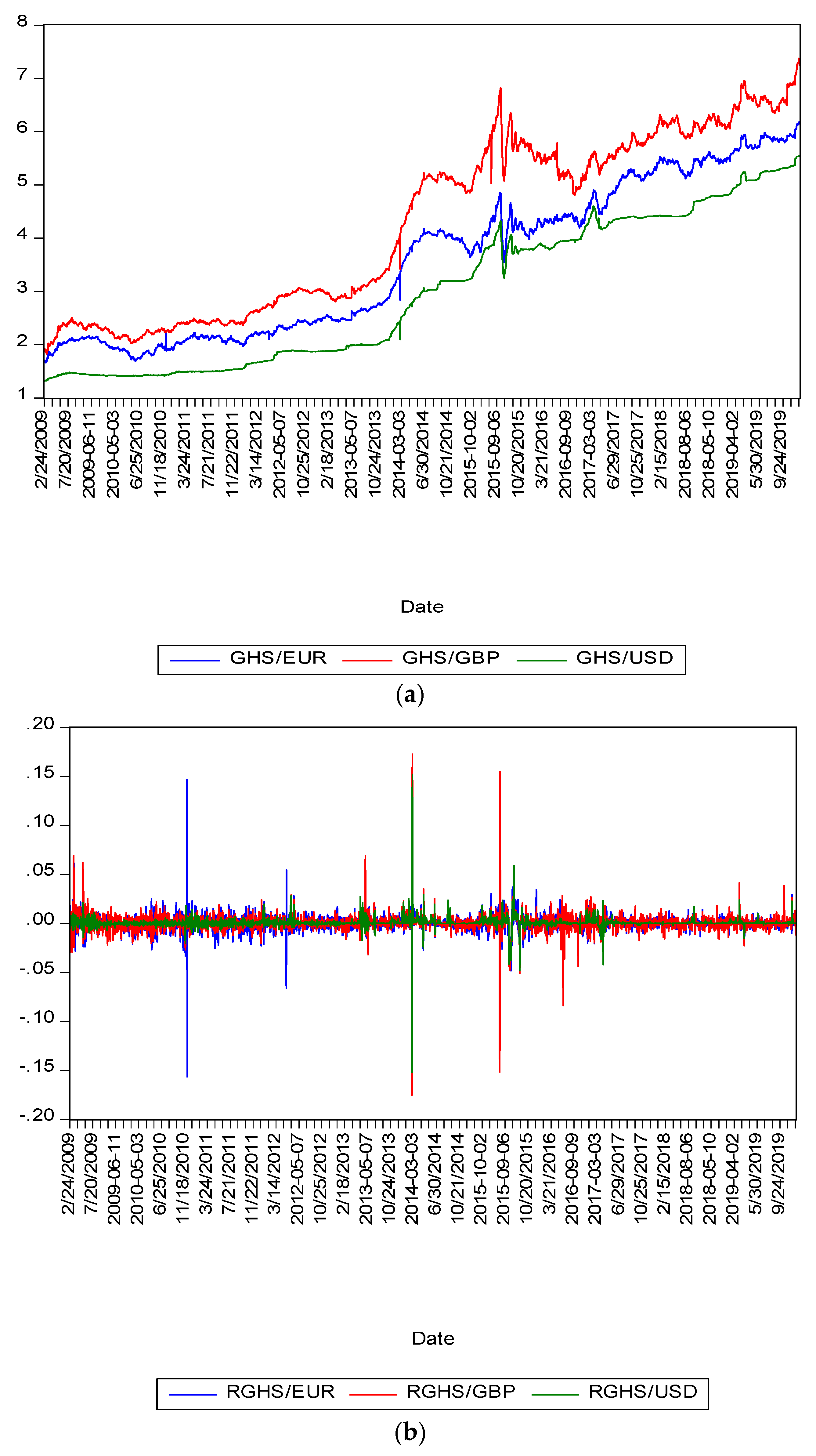
As a precursor to the summary statistics, we present in Figure 1 the plot of the Ghana Cedi to US dollar, Euro and Great Britain Pound exchange rate as well as the returns. A cursory look at the respective exchange rates in Figure 1a shows non-overlapping upward trends. This is an indication that the Ghana Cedi continuously depreciates against all major currencies in the long-run. The plots of returns presented in Figure 2 show similarity in returns even in times of extreme volatility especially for the US dollar and the Euro. To better understand the behavior of the exchange rates returns, we study the summary statistics of the returns.

The summary statistics of the exchange rate return series are shown in

Table 1. Descriptive statistics for exchange rates returns.

GHS/	Mean	Std. Dev.	Skewness	Kurtosis	Jarque-Bera	Q(2)	Q2(2)	ARCH-LM
EUR	0.00055	0.06574	−0.2465	1137.45	1.2835 × 108 *	567.98 *	593.96 *	791.18 *
USD	0.00061	0.03361	−0.0472	1103.06	1.2071 × 108 *	562.43 *	593.93 *	791.19 *
GBP	0.00056	0.13398	0.2266	820.34	6.6764 × 107 *	593.89 *	593.49 *	790.88 *

Notes: Data represent daily exchange rates returns spanning the period of 24 February 2009, to 19 December 2019. Std. Dev. is the standard deviation. Q(2) and Q²(2) refer to Ljung-Box statistic for serial correlation of order 2 in returns and squared returns. ARCH-LM is the Engle’s Lagrange multiplier statistic to test for heteroskedasticity computed using 20 lags. * indicates statistical significance at 5%.

. The mean percentage returns are all close to zero across all exchange rates and are small compared to the associated standard deviations. This signifies high exchange rates volatility, especially in GBP exchange rate return. Except for GBP that shows positive skewness value with lower kurtosis compared with both EUR and USD where their skewness values show negative with excess kurtosis, indicates the high probability of decreases in exchange rates returns. Also, the higher values of kurtosis seen across all exchange rates returns signify frequent extreme price changes. The Ljung-Box test confirms the presence of strong autocorrelation and the null hypotheses of normality of the returns distributions are strongly rejected by the Jarque-Bera statistic. The ARCH-LM test of Engle (1982) strongly confirms the presence of ARCH-effects in the individual return series and this is sufficient enough to employ GARCH models for the marginals. It is noticed in

Table 2. Unconditional Linear Correlation.

GHS/	EUR	USD	GBP
EUR	1
USD	0.0163	1
GBP	0.0136	0.0141	1

that the level of unconditional correlation of exchange rates returns are all positive but relatively low between all exchange rates pairs.

4. Empirical Results

4.1. Marginal Model Results

We began our analysis by first estimating the marginal models indicated by Equation (1) through to (3) before estimating the dependence model parameters (the copulas). Different combinations for lags values from one to three are taken to ensure the appropriateness of ARMA(k,m)-GARCH(p,q) specification with Student t-distribution for the marginals and a combination that gives minimum Akaike Information Criteria (AIC) value is selected as the best fit model.

The parameter estimates for the marginal distribution models are present in

Table 3. Parameter estimates for the marginal distribution model.

GHS/	EUR	USD	GBP
Mean Equation
${\varnothing }_0$	0.000438 *	0.000055 *	0.000249 *
	(0.000116)	(0.000013)	(0.000119)
${\varnothing }_1$	−1.282583 *	0.678063 *	0.911089 *
	(0.000156)	(0.029473)	(0.0211017)
${\varnothing }_2$	−0.994357 *	0.163287 *
	(0.000233)	(0.019986)
${\theta }_1$	1.281877 *	−0.741331 *	−0.929622 *
	(0.000249)	(0.024693)	(0.020039)
${\theta }_2$	0.994038 *
	(0.000137)
Variance Equation
${\alpha }_0$	0.000025 *	0.000007 *	0.000009 *
	(0.000003)	(0.000001)	(0.000001)
${\alpha }_1$	0.393398 *	0.375248 *	0.175997 *
	(0.063083)	(0.024909)	(0.006934)
${\beta }_1$	0.367484 *	0.623752 *
	(0.041624)	(0.017887)
${\beta }_2$			0.054972 *
			(0.01028)
${\beta }_3$			0.633581 *
			(0.006841)
Log-Likelihood	8430.102	11780.66	7663.246
Q(20)	0.66597	0.003332	0.1212
	[1.0000]	[1.0000]	[1.0000]
ARCH(20)	0.0014332	0.0015125	0.006177
	[1.0000]	[1.0000]	[1.0000]
Shapiro-Wilk	0.051559	0.052169	0.038803
	[0.0000]	[0.0000]	[0.0000]
Jarque-Bera	1.2833 × 108	1.1453 × 108	6.6767 × 107
	[0.0000]	[0.0000]	[0.0000]

Notes: The table shows parameter estimates for the marginal models in Equations (1)–(3) with standard errors in brackets and p-values in square brackets. p-values less than 0.05 indicate rejection of the null hypothesis. * represents statistical significance at the 5% level. Q(20) is the Ljung-Box statistics computed using 20 lags for serial correlation in the residual models. ARCH is Engle’s LM test for the ARCH effect in the residual up to 20th order. Shapiro-Wilk and Jarque-Bera tests test for normality of standardized residuals.

. The results presented in Table 3 show that a GARCH (1,1) model accurately captures the volatility dynamics of EUR and USD exchange rates returns while the dynamics of the GBP exchange rate return volatility is well captured by a GARCH (1,3) model. Various model diagnostic tests (goodness-of-fit test) for the marginals including the Ljung-Box and ARCH-LM tests as well as normality test based on Shapiro-Wilk and Jarque-Bera tests are performed. The Ljung-Box statistic and the ARCM-LM statistic respectively indicate that there is no serial correlation in the residuals of the marginals and absence of ARCH effects remaining in the residuals. On the other hand, both normality tests results indicate that the distribution of the residuals deviates from normality. Notwithstanding, the choice of using copula models is so appropriate to capture dependencies between exchange rates returns pairs because the goodness-of-fit test results indicate that the marginal distribution models are correctly specified. Therefore, the best fitting marginal models based on AIC are ARMA (2,2)-GARCH (1,1) for EUR exchange rate return, ARMA (2,1)-GARCH (1,1) for USD exchange rate return and ARMA (1,1)-GARCH (1,3) for GBP exchange rate return.

4.2. The Copula Models Results

Table 4. Estimates for Time-Invariant Bivariate Copula Models.

Copula Models	EUR-USD	EUR-GBP	USD-GBP
Gaussian copula
$\rho$	0.3866 *	0.6689 *	0.3872 *
	(0.016)	(0.009)	(0.016)
AIC	−379.1791	−1399.383	−380.6324
Student-t copula
$\rho$	0.3389	0.6824	0.3533
	(0.022)	(0.012)	(0.021)
ϑ	2.8801 *	3.6819 *	3.3945 *
	(0.253)	(0.368)	(0.345)
AIC	−534.009	−1598.632	−496.1728
Gumbel copula
$\delta$	1.341 *	1.884 *	1.343 *
	(0.021)	(0.032)	(0.021)
AIC	−480.3786	−1497.994	−485.5223
Rotated Gumbel copula
$\delta$	1.302 *	1.845 *	1.295 *
	(0.02)	(0.031)	(0.02)
AIC	−386.6807	−1403.206	−364.8547
Clayton copula
$\alpha$	0.5647*	1.221*	0.5816*
	(0.034)	(0.044)	(0.035)
AIC	−267.1438	−1116.208	−239.6604
Rotated Clayton copula
$\alpha$	0.5986 *	1.349 *	0.6118 *
	(0.035)	(0.046)	(0.035)
AIC	−423.8038	−1267.054	−434.7387

Notes: The table displays parameter estimates for different static copula models for each currency pair shown in each column. Standard error values are in brackets and * indicates statistical significance at the 0.05 level. Each copula model’s AIC (Akaike information criterion) value is shown. In all AIC values in “bold” indicate minimum values that recommend the best-fit copula model (Student-t copula).

reports the estimates of time-invariant copula for all the exchange rate returns pairs.

The parameter estimates for all the copula families used in this study show positive dependence for all the exchange rates returns pairs. Since the parameter estimates for the Gaussian and Student-t copulas measure the dependence between exchange rates returns pairs, we can then infer from Table 4 that the EUR-GBP exchange rates returns pair exhibit strong dependence with higher conditional correlation coefficient estimate ($\rho$), while there are moderate dependencies between EUR-USD and USD-GBP exchange rates returns pairs. The estimates of Gaussian and Student-t time-invariant parameters are all significant at the 5% level. The estimates of time-invariant parameters of Archimedean copulas used in this study such as Gumbel (rotated Gumbel) and rotated Clayton (Clayton) copulas capture upper (lower) tail dependencies and are all significant at the 5% level, as shown in Table 4. It can be inferred from Table 4 that parameter estimates for Gumbel and rotated Clayton copulas are higher than their corresponding counterparts (rotated Gumbel and Clayton). This result is consistent in the literature, that exchange rates tend to jointly depreciate more than they appreciate together. For all exchange rates returns pairs, there is higher extreme co-movement or tail dependence between the EUR-GBP pair than the EUR-USD and USD-GBP pairs but all pairs show positive dependence. In all, the Student-t copula for time-invariant copula models provides a better fit for all exchange rates returns pairs based on the AIC model selection criterion adopted for this study. This indicates that exchange rates markets boom and crash together.

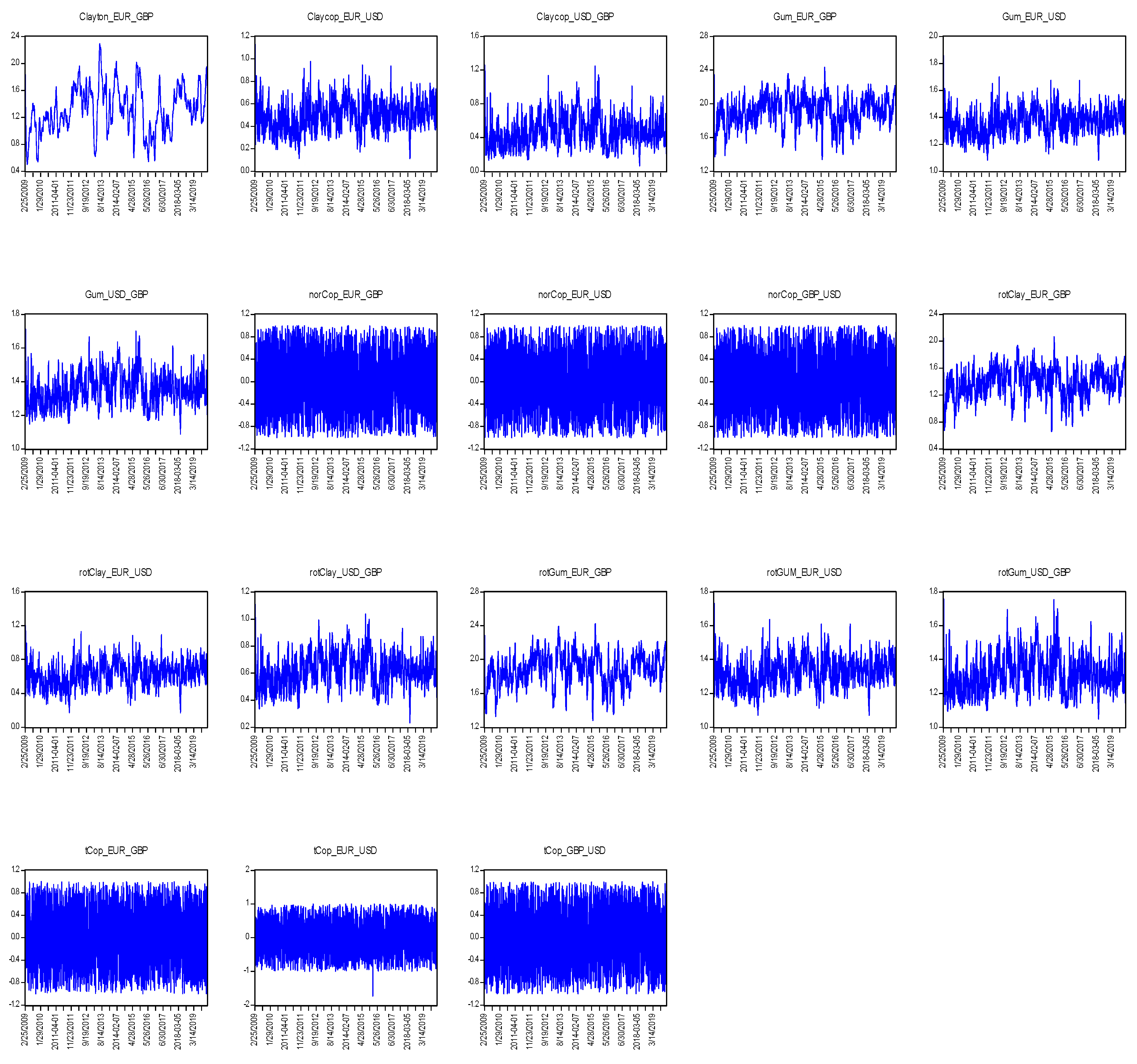
The results of time-varying copula model parameters shown in

Table 5. Estimates for Time-Varying Bivariate copula models.

Copula Models	EUR-USD	EUR-GBP	USD-GBP
TVP-Gaussian
${\mathsf{\Psi }}_0$	0.0412 *	0.0213 *	−0.0047
	(0.00601)	(0.00587)	(0.00594)
${\mathsf{\Psi }}_1$	0.4532 *	0.6253 *	0.1025
	(0.01314)	(0.01327)	(0.01316)
${\mathsf{\Psi }}_2$	−2.3641 *	1.7841 *	1.4352
	(0.00589)	(0.00595)	(0.0059)
AIC	−430.23	−1405.42	−411.59
TVP-Student-t
${\mathsf{\Psi }}_0$	0.0384 *	0.0241 *	−0.0063
	(0.0059)	(0.0058)	(0.00593)
${\mathsf{\Psi }}_1$	0.5461 *	0.6562 *	0.1465
	(0.0058)	(0.0134)	(0.01335)
${\mathsf{\Psi }}_2$	1.7563 *	2.3641 *	1.6343
	(0.0061)	(0.0059)	(0.00595)
AIC	−567.89	−1604.36	−546.73
TVP-Clayton
${\mathsf{\Psi }}_0$	−0.2578 *	0.1115 *	0.2931 *
	(0.00582)	(0.00582)	(0.00596)
${\mathsf{\Psi }}_1$	−0.7775 *	0.9273 *	−0.6219 *
	(0.0026)	(0.007)	(0.0036)
${\mathsf{\Psi }}_2$	−6.3813 *	−0.5998 *	−8.3688 *
	(0.00592)	(0.00587)	(0.00595)
AIC	−293.4	−1167.26	−285.35
TVP-rotated Clayton
${\mathsf{\Psi }}_0$	0.0695 *	1.0452 *	−0.1654 *
	(0.00588)	(0.00594)	(0.00599)
${\mathsf{\Psi }}_1$	−0.7163 *	−0.3841 *	−0.5982 *
	(0.0029)	(0.0044)	(0.0024)
${\mathsf{\Psi }}_2$	−5.5725 *	−4.6319	−4.2662
	(0.00593)	(0.00589)	(0.00601)
AIC	−437.17	−1291.99	−442.99
TVP-Gumbel
${\mathsf{\Psi }}_0$	0.5544 *	1.5418 *	0.498 *
	(0.00599)	(0.006)	(0.00598)
${\mathsf{\Psi }}_1$	−0.7515 *	−0.1367 *	−0.5607 *
	(0.0019)	(0.0036)	(0.0019)
${\mathsf{\Psi }}_2$	−6.5229 *	−5.292 *	−5.9222 *
	(0.00597)	(0.00589)	(0.00599)
AIC	−498.76	−1535.04	−501.56
TVP-rotated Gumbel
${\mathsf{\Psi }}_0$	0.3416 *	1.0423 *	0.683 *
	(0.00596)	(0.00602)	(0.00585)
${\mathsf{\Psi }}_1$	−0.7469 *	0.2711 *	−0.6123 *
	(0.0017)	(0.0039)	(0.0022)
${\mathsf{\Psi }}_2$	−6.5702 *	−3.923 *	−7.875 *
	(0.00591)	(0.00592)	(0.00581)
AIC	−405.02	−1447.03	−391.54

Notes: The table displays parameter estimates for different time-varying copula models for each currency pair shown in each column. Standard error values are in brackets and * indicates statistical significance at the 0.05 level. Each copula model’s AIC (Akaike information criterion) value is shown. In all, AIC values in “bold” indicate minimum values that recommend the best-fit copula model (Student-t copula).

indicate that all the time-varying copula models perform better than their static counterparts based on the AIC model selection criterion. Consistent with the static models, the Student-t copula model provides a better fit for all pairs than the other models considered in the study with minimum AIC value. However, the choice of Student-t copula shows that exchange rates jointly depreciate and appreciate together, the Gumbel and rotated Clayton copulas outperformed their respective counterparts (rotated Gumbel and Clayton), indicating that exchange rates tend to jointly depreciate more than appreciate. The evolution of dependence and tail dependence copula parameters is evidenced in Figure 2. The time-varying Student-t copula that provides a better fit for all pairs, exhibits or is akin to a white noise process, as well as the time-varying Gaussian copula. The dynamic Archimedean copulas considered in this study show greater upper tail dependence than the lower tail, suggesting the presence of asymmetry in the bivariate relationships. Notwithstanding this, the better fit Student-t copula model reveals that the major trading currencies in Ghana jointly depreciate and appreciate against the GHS. In other words, whenever the GHS’s value drops (rises), the foreign currencies jointly rise (drop) in value. This can be attributed to the high integration and efficiency of exchange rate markets of developed economies like the US, UK and the Euro Zone. Integrated markets tend to move together and any disequilibrium is quickly restored to limit speculator from making arbitrage profit. From the demand side, the US dollar, the Euro and Great Britain pound as currencies for international business are near-perfect substitutes, though US dollar leads. Therefore, in times of high demand for foreign currencies, any of these is susceptible to demand pressure and hence joint depreciation/appreciation against the cedi.

The findings imply that there is no opportunity for international currency diversification from the three major currencies. It is also worthless for market players, speculators, importers and currency traders to hoard the USD in an anticipation of extreme depreciation of the GHS against the USD. As evidenced by our study results, the foreign currency pairs with the GHS co-move in both directions (depreciation and appreciation) and the co-movement is more prevalent in harsh extreme market conditions. Therefore, the focus should not only be on the USD to cause unnecessary pressure on the USD in anticipation of the GHS losing ground to the USD (GHS depreciating against the USD) but the focus should rather be on all the major trading foreign currencies, especially the GBP and the EUR.

4.3. Comparing Time-Varying Copula Models with DCC-GARCH Model

We compare the copula results with a multivariate GARCH model with dynamic conditional correlation (DCC) proposed by Engle (2002) where time-varying conditional correlations are driven by the cross product of the lagged standardized residuals and an autoregressive term. This model assumes that returns of n assets are conditionally multivariate normal with zero expected value and covariance matrix H_t. The estimation procedures of DCC-GARCH is like copula model estimation whereby the GARCH parameters for the individual series (marginal distributions) are estimated first, followed by estimating the parameters driving the correlation dynamics (see Tse and Tsui 2002). The DCC-GARCH model has been widely applied to financial phenomena (see Engle and Colacito 2006; Lee 2006; Coudert and Gex 2010; Cai et al. 2016).

In this study, we consider DCC (1,1)-GARCH (1,1) model. Given the information set ${\eta }_{t-1}$ available at time t − 1 of the return r_t of an asset is distributed as $r_t/{\eta }_{t-1}\backsim N\left(0,H_t\right)$ with

$$H_t=D_t{R}_t{D}_t$$

(17)

where $D_t=diag\left\{\sqrt{h_{it}} \right\}$ is $n\times n$ diagonal matrix of the time-varying conditional standard deviation of Standardized residual $z_t$ at time t,$R_t={\left\{{\rho }_{ij}\right\}}_t$ is $n\times n$ conditional symmetric correlation matrix of $z_t$ at time t.

The dynamics of the correlation in the DCC (1,1)-GARCH (1,1) model is expressed as

$$Q_t=\left(1-a-b\right)\overline{Q}+a{z}_{t-1}{z^{\prime }}_{t-1}+b{Q}_{t-1}$$

(18)

where

$a\ge 0, b\ge 0$ and $a+b<1$,

$Q_t$ is the $n\times n$ time-varying covariance matrix of $z_t$,

$\overline{Q}$ is the $n\times n$ unconditional covariance matrix of $z_t$.

The model parameters are estimated following the two-stage maximum likelihood estimation procedure proposed by Engle (2002) and, Tse and Tsui (2002).

The results for the DCC (1,1)-GARCH (1,1) model are presented in

Table 6. Estimation results from the bivariate DCC(1,1)-GARCH(1,1) model.

Panel A: Marginal Model Results
GHS/	EUR	USD	GBP
Variance equation
${\alpha }_0$	0.000012 *	0.0000001	0.000004 *
	0.000001	0.000024	0.000001
${\alpha }_1$	0.21585 *	0.228549 *	0.074432 *
	0.05652	0.039065	0.022583
${\beta }_1$	0.660569 *	0.770451 *	0.877705 *
	0.061083	0.340935	0.008594
Panel B: Bivariate DCC results
GHS/	EUR-USD	EUR-GBP	USD-GBP
$\rho$	0.005637 *	0.012417 *	0.002025 *
	0.00000005	0.00000006	0.00000002
$a$	0.010367 *	0.000001	0.005039
	0.002584	0.000127	0.003424
$b$	0.9836 *	0.902889 *	0.990627 *
	0.007146	0.108864	0.007068
AIC	309.86	132.03	408.26

Notes: The table displays parameter estimates of DCC (1,1)-GARCH (1,1) models for each currency pair shown in each column. Standard error values are in brackets and * indicates statistical significance at the 0.05 level. The AIC (Akaike information criterion) value for DCC for each currency pair is shown.

. The results show that apart from the constant parameter ${\alpha }_0$ in the univariate GARCH model for GHS/USD return series, all the estimated GARCH model parameters (${\alpha }_1, and {\beta }_1)$ are statistically significant.

We can infer from these results that the conditional variance of exchange rate return is influenced by past return innovation and by its lagged variance. The parameters $a$ and $b$ of the DCC (1,1) model respectively capture the effects of standardized lagged shocks $(z_{t-1}{z^{\prime }}_{t-1})$ and the lagged dynamic conditional correlation effects $Q_{t-1}$ on current dynamic conditional correlation. It is worth noting that the existent of time-varying dynamic correlations are determined by the statistical significance of the coefficients $a$ and $b$ in each pair of the exchange rates returns. Though the results show that the coefficient $a$ is not significant for both EUR-GBP and USD-GBP pairs except for EUR_USD pair, $b$ is highly significant and positive for all exchange rate pairs and close to 1. This indicates that time-varying dynamic correlations exist and therefore, Bollerslev et al.’s (1988) constant conditional correlation cannot be assumed. The average conditional correlation $\rho$ for all pairs as reported in Table 6 [EUR-USD(0.005637), EUR-GBP(0.012417), USD-GBP(0.002025)], is significant and positive as well and it should be noted that the low average conditional correlation values between all pairs show no extreme co-movement between the exchange rate pairs.

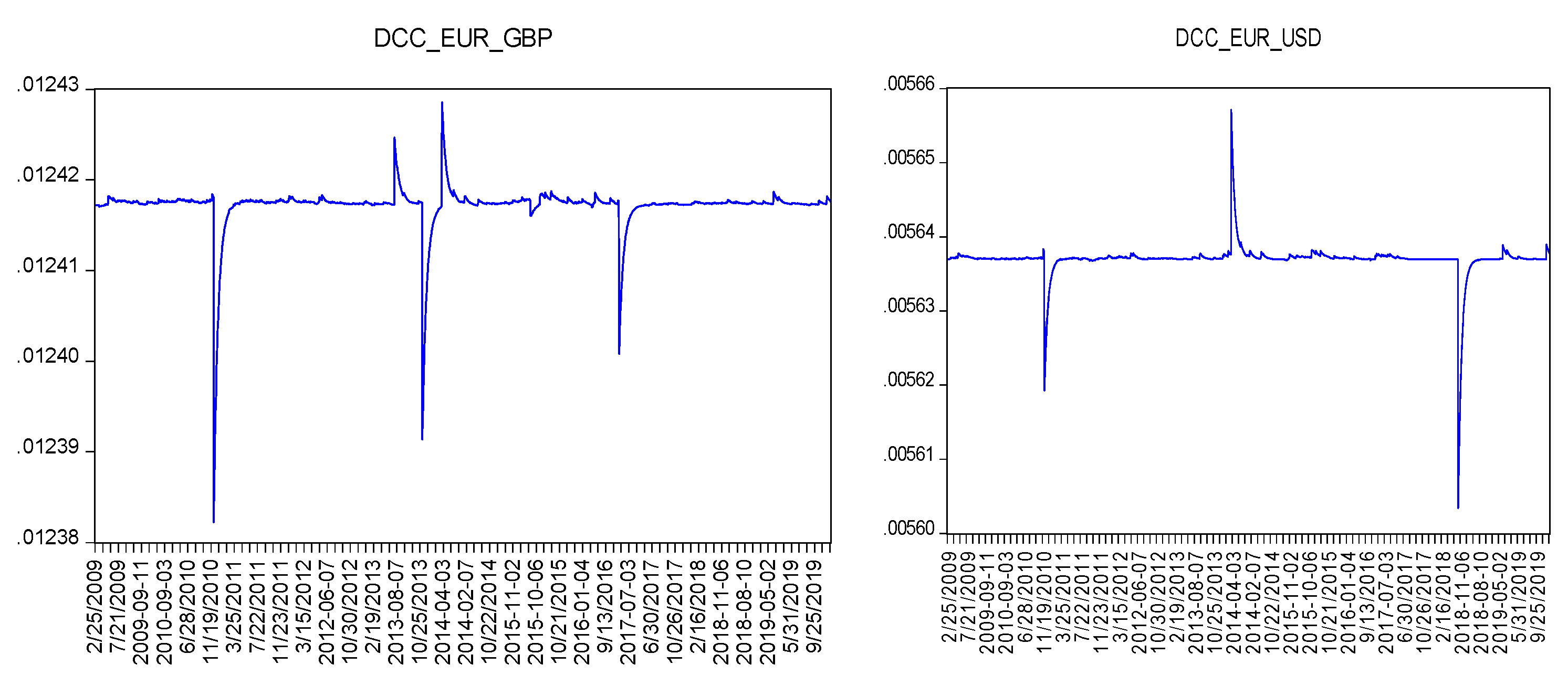
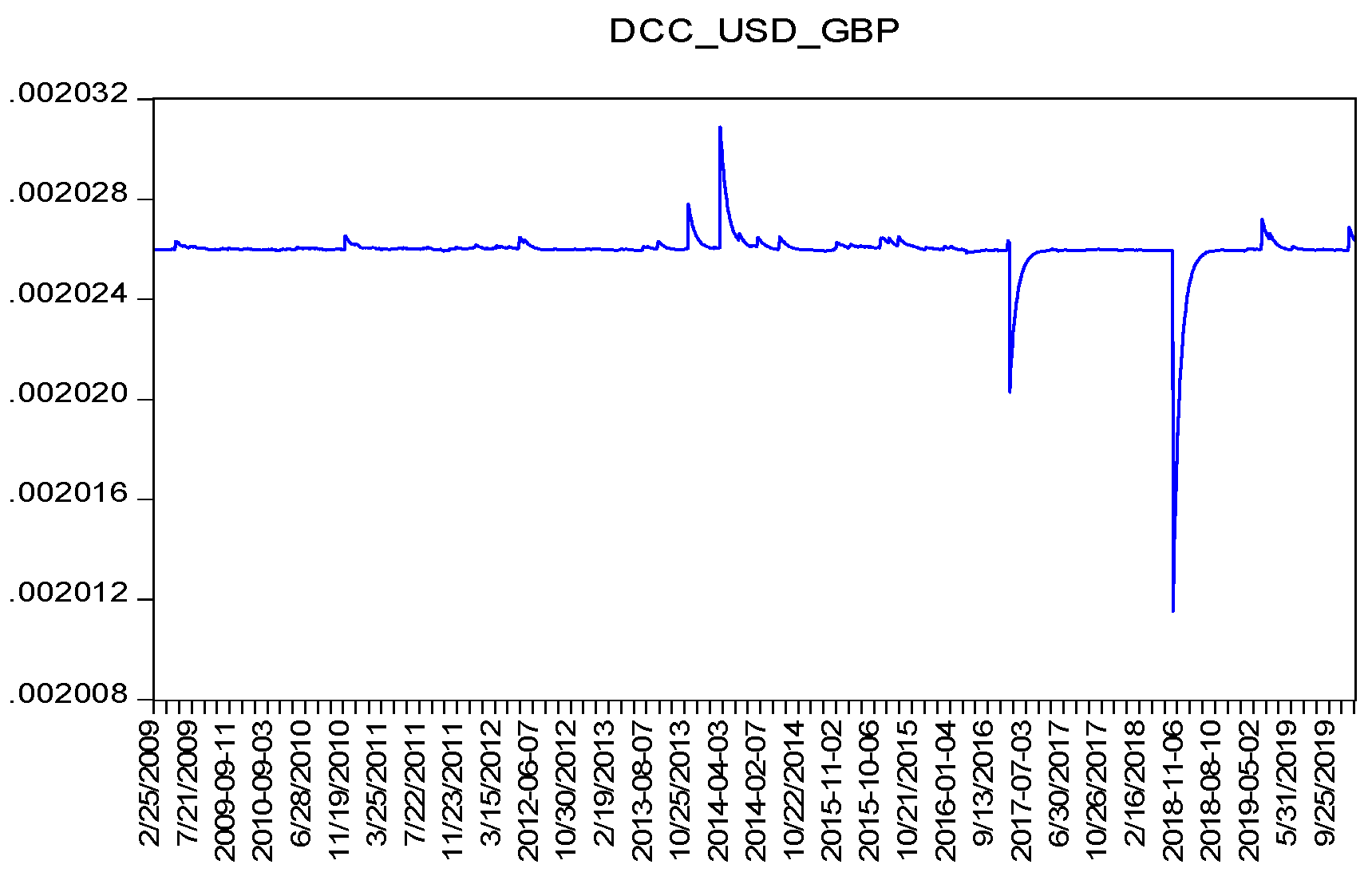
A visual presentation of correlation dynamics between the exchange rate return pairs is shown in Figure 3 using the DCC (1,1)-GARCH (1,1) modeling framework. By observing the evolution of these correlations, we identify marginal fluctuations in the correlation dynamics with occasional big fluctuations either above or below the average, which usually occur close to the beginning or the terminating periods of the incidental periods. Even though the correlation fluctuations are marginal over a wide range of the study period, the existence of peaks and troughs occurring around the beginning and the terminating periods of the incidental periods justify the dynamic nature of the conditional cross-correlations.

It is interesting to note that both DCC and copula models provide evidence of time-varying co-movements between the exchange rate pairs, the DCC model shows high persistence of correlations which is evidenced by the fact that the DCC parameter $b$ is near 1 for all exchange rate pairs. This high persistence may push away a long-run average of the correlation for a considerable long period by shocks, thereby failing to detect extreme co-movement between the exchange rate pairs which is the main purpose of our study. Moreover, the complexity involves in constructing multivariate distribution by decomposing it into dependence structure and marginal distributions using a DCC model framework that makes the use of copulas, which are more flexible for achieving such a task and making them a preferred model to the DCC model.

5. Conclusions

Excessive demand for foreign currency always disadvantages the domestic currency, causing the domestic currency to fall in value against the foreign currency. The recognition that currency markets move together, especially more at extreme market conditions, will help reduce the excessive pressure that is usually brought to bear on the domestic currency in pursuit of foreign currency to cause drastic depreciation of the domestic currency against the highly demanded foreign currency. To ascertain the joint depreciation and appreciation of foreign currencies against the GHS at extreme market conditions on Ghana’s foreign exchange market, this paper examines the dependence structure between the EUR-USD, USD-GBP and EUR-GBP pairs with each currency expressed as a unit in GHS term, using daily data from 24 February 2009 to 19 December 2019. To determine the degree of the dependence and tail dependence structure between the exchange rates pairs, we use six different copula functions including Gaussian, Student-t, Clayton, Gumbel, rotated Clayton and rotated Gumbel copulas. The results show positive dependence between the exchange rates pairs and the tail dependences are symmetrical and evolve (time-varying). Among all the copula families considered in our study, student-t copula provides a better fit for both static and time-varying copulas based on AIC, indicating and consistent with literature that exchange rate markets boom and crash together at extreme market conditions. Notwithstanding this, the Archimedean copulas provide evidence of upper tail dependence.

The study also compares the copula results to DCC(1,1)-GARCH(1,1) model by examining the joint movement between exchange rate pairs in a multivariate sense. The multivariate DCC-GARCH results show marginal fluctuations of correlations over a wide range of the study period with occasional big fluctuations close to the beginning and terminating periods of the incidental periods and these confirm the presence of dynamic conditional correlation between the currency pairs. Moreover, the DCC-GARCH model results show high persistence in correlation dynamics, leading to its inability to capture extreme co-movement between the exchange rate pairs. Notwithstanding the DCC multivariate’s appeal to modeling volatility transmission across financial time series, the complexity involves in constructing multivariate distribution by decomposing it into dependence structure and marginal distributions using the DCC model framework makes the use of copulas more appealing to modeling dependence structure between exchange rate pairs.

We observe through the copulas that the three major currencies jointly depreciate/appreciate under extreme harsh conditions This finding provides lessons to be drawn from by investors, importers, currency market players, speculators and the general public as a whole that there is no point in rushing out in a panic for the USD in an anticipation of the domestic currency (GHS) depreciating highly against the USD because, in such situations, all the other foreign currencies and the USD jointly appreciate. The activity of benefiting from international currency diversification is non-existing. The finding of the joint movement of the major currencies provides policymakers with useful information for managing exchange rate risk in the extreme period. Specifically, monetary authorities should continuously monitor activities of these three currencies and implement appropriate interventions against shocks from any of the countries to stabilize the cedi.