Copula Model Selection for Vehicle Component Failures Based on Warranty Claims

Abstract

In the automotive industry, it is important to know whether the failure of some car parts may be related to the failure of others. This project studies warranty claims for five engine components obtained from a major car manufacturer with the purpose of modeling the joint distributions of the failure of two parts. The one-dimensional distributions of components are combined to construct a bivariate copula model for the joint distribution that makes it possible to estimate the probabilities of two components failing before a given time. Ultimately, the influence of the failure of one part on the operation of another related part can be described, predicted, and addressed. The performance of several families of one-parameter Archimedean copula models (Clayton, Gumbel–Hougaard, survival copulas) is analyzed, and Bayesian model selection is performed. Both right censoring and conditional approaches are considered with the emphasis on conditioning to the warranty period.

1. Introduction

Studying the reliability of complex engineering systems, one has to account for possible failures of their components. Some reliability models assume the independence of individual component failures, which is a nice simplification, reducing the reliability analysis of the system to the reliability analysis of its components (Trivedi 2008). It is convenient to study component reliabilities in terms of random variables measuring the time-to-failure (TTF) for individual components (Suzuki et al. 2001; Trivedi 2008).

However, more adequate models would address the dependence between the component failures, which may be caused by different factors, such as:

• simultaneous failures of two or more components caused by a common event;
• long-term maintenance and exploitation conditions shared by the entire system causing excessive wear and tear of all its components;
• failure of one component putting other components under additional pressure and causing their excessive wear and tear.

These three factors of dependence have been identified and well documented in the life insurance literature addressing multiple life policies (Frees et al. 1996; Hardy and Li 2011; Shemyakin and Youn 2006), as common disaster, common lifestyle, and broken-heart syndrome. Each of these factors can be introduced to reliability studies via such tools as proportional hazard models, competing risk models, or correlation analysis (Kotz et al. 2004; Lai and Lin 2006). However, none of these models is particularly effective at addressing all three factors simultaneously.

Copula models of dependence are becoming increasingly popular in such diverse fields as insurance, finance, and health studies because they make it possible to address all three above-mentioned factors of dependence in one general framework (Joe 2014). This framework is provided by modeling the entire joint distribution of individual TTF variables using special classes of copula functions. Copula models have the advantage of being able to address complex non-linear dependence structures going beyond correlation analysis (Embrechts et al. 2003) and to model successfully the tails of the joint TTF distribution corresponding to the catastrophic events of cascade failures, playing a special role in engineering system control and risk management. However, misspecification of a copula model (using an inadequate class of copulas) may lead to gross underestimation of risks, as was illustrated by the recent role of Gaussian copula models in the credit derivative crisis (Salmon 2012). Thus, special attention should be paid to an adequate choice of the class of copula models to be used in a specific application.

Automobiles are good examples of complex engineering systems, where the three above-mentioned factors play an important role in most of the failures of the system components (Baik et al. 2004; Heyes 1998). Car manufacturers and dealers, as well as automobile insurers and warranty providers should be interested in realistic models describing related component failures as they help to predict the risks and costs related to these failures. Using warranty claim data, one can build predictive models of failure rates and failure distributions of auto parts (Kalbfleisch et al. 1991; Lawless 1998; Lawless et al. 1995).

The present paper extends the results of (Kumerow et al. 2014) presented at the World meeting of International Society for Bayesian Analysis in Mexico (ISBA-14) and an example presented in (Shemyakin and Kniazev 2017) illustrating the comparison of copula families. We focus on the characterization of the dependence between TTF distributions of related vehicle parts. Analyzing the warranty claim data provided by a major car manufacturer (Baik 2010), we construct copula models for the joint TTF distribution of ten pairs of automotive components responsible for the majority of the repair/replacement costs. For each of the four classes of copulas analyzed in the paper, we provide Bayes estimates of the parameter of association, determining the strength of dependence. Both the right censoring scheme and conditioning to the observation period are considered. A comparison of the relative performance of four classes of copulas is provided. Emphasis is made on the model selection involving the Bayesian approach introduced in (Bretthorst 1996) and further developed in (Huard et al. 2006). Bayesian procedures are implemented via Markov chain Monte Carlo and Monte Carlo sampling from the prior.

Section 2 of the paper contains a description of the entire dataset and five critical components analyzed in the sequel. Section 3 is dedicated to the general description of the copula models and four specific classes of copulas chosen for further analysis. Section 4 summarizes the results of parametric estimation for four chosen classes of copulas. In Section 5, the comparison of the best fitting models in each class is discussed using information criteria, Kolmogorov–Smirnov statistics, and tail dependence. Section 6 describes the procedure of Bayesian model selection and the estimation of posterior probabilities determining the final choice of the model. Section 7 contains a brief discussion of the t-copula construction for dimensions higher than two.

2. Data Description

2.1. Hyundai Warranty Claims

Vehicle manufacturers do not have to make their failure reports public, and historically, very few data have been made available for statistical analysis. Warranty claims present a unique opportunity to record early failures and make conclusions on the reliability of separate vehicle components and the relationships between the failures of these components and their assemblies. We will use the open source data presented by Hyundai, including a dataset of 58,029 manufacturer warranty claims on the Hyundai Accent from 1996 to 2000. A more detailed description of the dataset is available in one of the examples introduced in (Shemyakin and Kniazev 2017). We focus primarily on the variable “time to failure” (TTF), which indicates the time (in days) from sales to repair. In (Baik 2010), the author addressed the distribution models for this variable measured for various components, performing a preliminary analysis of each component repaired. In that study, all failures were treated as independent events. However, the author concluded that TTF variables for various components were likely to be associated. Our goal is to model this association.

2.2. Engine Assembly Components

Five main components that most frequently failed and caused warranty claims were chosen in (Kumerow et al. 2014; Shemyakin and Kniazev 2017) out of the available list of 60: the spark plug assembly (A), ignition coil assembly (B), computer assembly (C), crankshaft position sensor (D), and oxygen heated sensor (E). The spark plug assembly brings power to the spark plug, which provides the spark for the motor to start. The ignition coil assembly regulates the current to the spark plugs, helping to ignite the spark. The computer assembly includes engine sensors, and it controls the electronics for fuel-injection emission controls and the ignition. The crankshaft position sensor controls ignition system timings and reads rpms. Finally, the oxygen heated sensor determines the gas-fuel mix ratio by analyzing the air from the exhaust and adjusting the ratio as needed. The latter two components are controlled by the computer assembly. A failure of one of the chosen components does not necessarily cause the other ones, yet all of these components are all closely related and could all need to be repaired or replaced if, for example, a single event caused the system to short out.

Records were available only for 32,667 cars from the dataset that had at least one of the five main components fail within the time frame of the warranty. However, this dataset is somewhat limited due to the fact that many cars did not experience failure of those parts within the warranty years. It would be desirable to include all cars, whether or not they had one of the main five components fail. Using full data would help us make the models for joint dependence more realistic; however, such a dataset is also more complicated to obtain. Thus, our main focus is on the cars for which component failures were registered. In the case of multiple repairs, only the date of the first repair of each component per vehicle was used, and all repeats were excluded.

A simultaneous failure of two or more components might indicate that in the course of diagnostics, a repair or replacement of several parts was recommended, and each of these parts was recorded as failing. The most important goal of the study is to be able to predict the failures of components based on the history of other components’ failure during the warranty period. The emphasis is made on joint failures happening early or late in the warranty period.

The ultimate goal of this paper is to suggest models for the joint distribution of times-to-failure of different pairs of components. We focus on the pairwise associations. It is established that the time-to-failure for an individual component can be effectively fitted to a parametric model (Baik 2010; Wu et al. 2000); thus, we will use full parametric modeling of the marginal distributions of individual components. In (Shemyakin and Kniazev 2017), non-parametric analysis of the marginal was considered.

Notice also that with the warranty period for all cars in the sample being the same five years, we may either want to consider all 32,667 cars in the dataset (some cars had several claims) as providing right censored data (I) (Schemper et al. 2013) or consider for each pair of components only the cases when both components fail during the warranty period, which represents conditioning to failure events in the warranty period (II) (Shemyakin and Kniazev 2017). The first approach uses more complete information from the data, but with the extremely high percentage of censored observations (repairs are relatively rare events), it may also lead to erroneous values of correlation and tail dependence, thus misrepresenting the dependence structure. In particular, right tails corresponding to joint failures late in the warranty period, which might be of a special concern to the manufacturer, will not be captured with the censoring approach. In the meantime, the second approach may also overestimate the actual association between two TTF variables. In our context, we are mostly interested in related failures occurring during the warranty period. As we will see from the comparison of these two approaches in Section 4, right censoring may not provide adequate models for such instances, and we recommend the second (conditional) approach for model selection in Section 5 and Section 6. In Section 7, we will return to the first approach to discuss parametric estimation for more general five-dimensional models. This is necessitated by the fact that the failure of all five or even four components during the warranty period is an extremely rare event, and we did not have enough data to apply the second approach in higher dimensions.

Table 1. Number of registered failures.

Component	All	A	B	C	D	E
A	1883		467	441	152	307
B	1745			260	160	258
C	1646				271	686
D	1860					267
E	10,178

contains the sample sizes characterizing the counts of individual failures of the components (column “All”) and related failures of their pairs (Rows A–E, Columns B–E), registered during the warranty period.

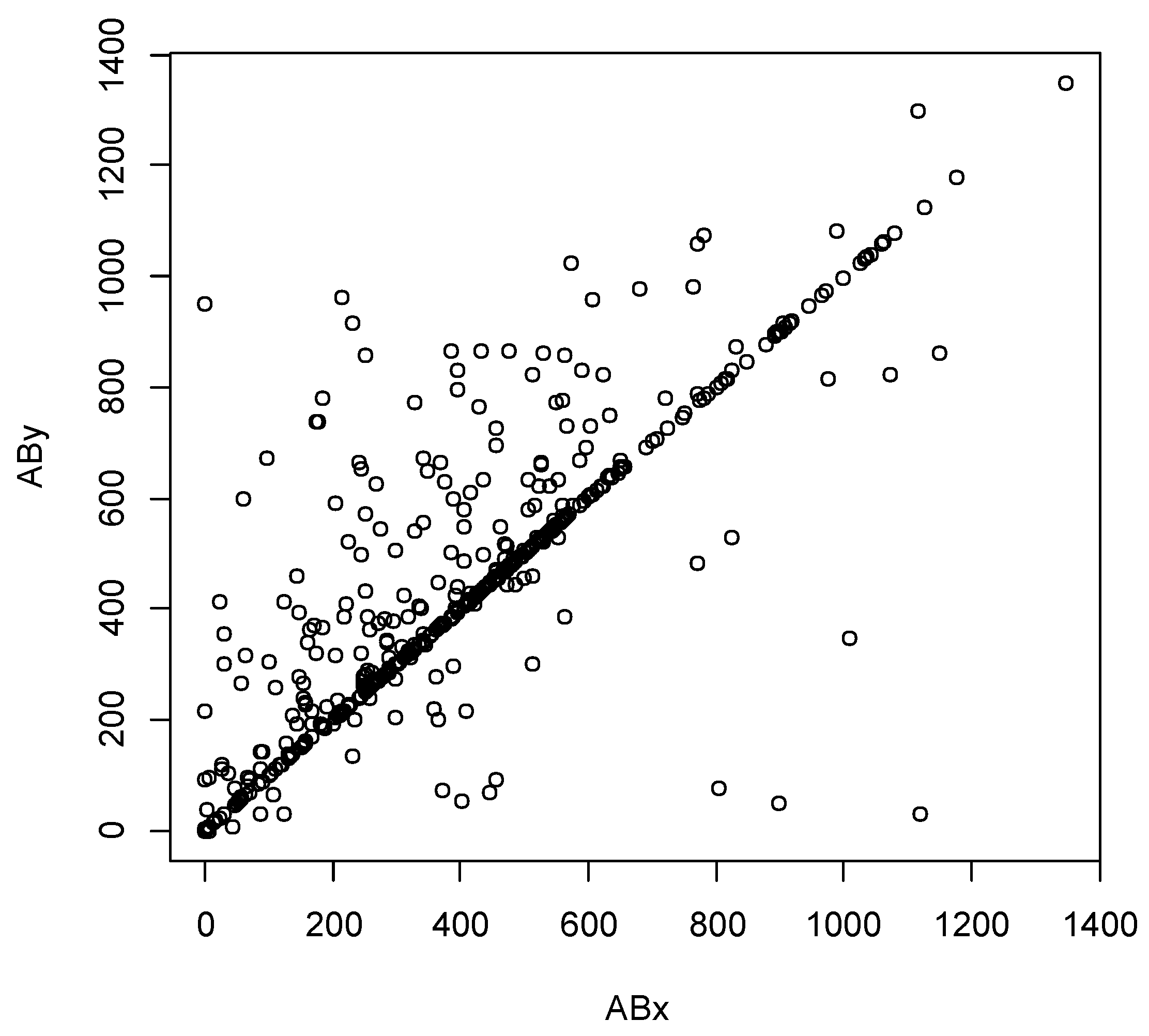
The scatterplots in Figure 1 and Figure 2 show the TTFs of one part versus the TTFs of another, given in days. The first scatterplot in Figure 1 displays TTFs for the pair A and B, which exhibits the highest degree of dependence including multiple simultaneous failures (points on the main diagonal). That may correspond to the close functional relationship between the spark plug assembly (A) and ignition coil assembly (B), which results in the general recommendation to repair (replace) these parts simultaneously in the case of a failure of one of them. Notice a linear diagonal pattern in the upper right quadrant indicating upper tail dependence and, to a lesser extent, a similar diagonal pattern in the lower left quadrant suggesting lower tail dependence (to be further discussed in Section 3).

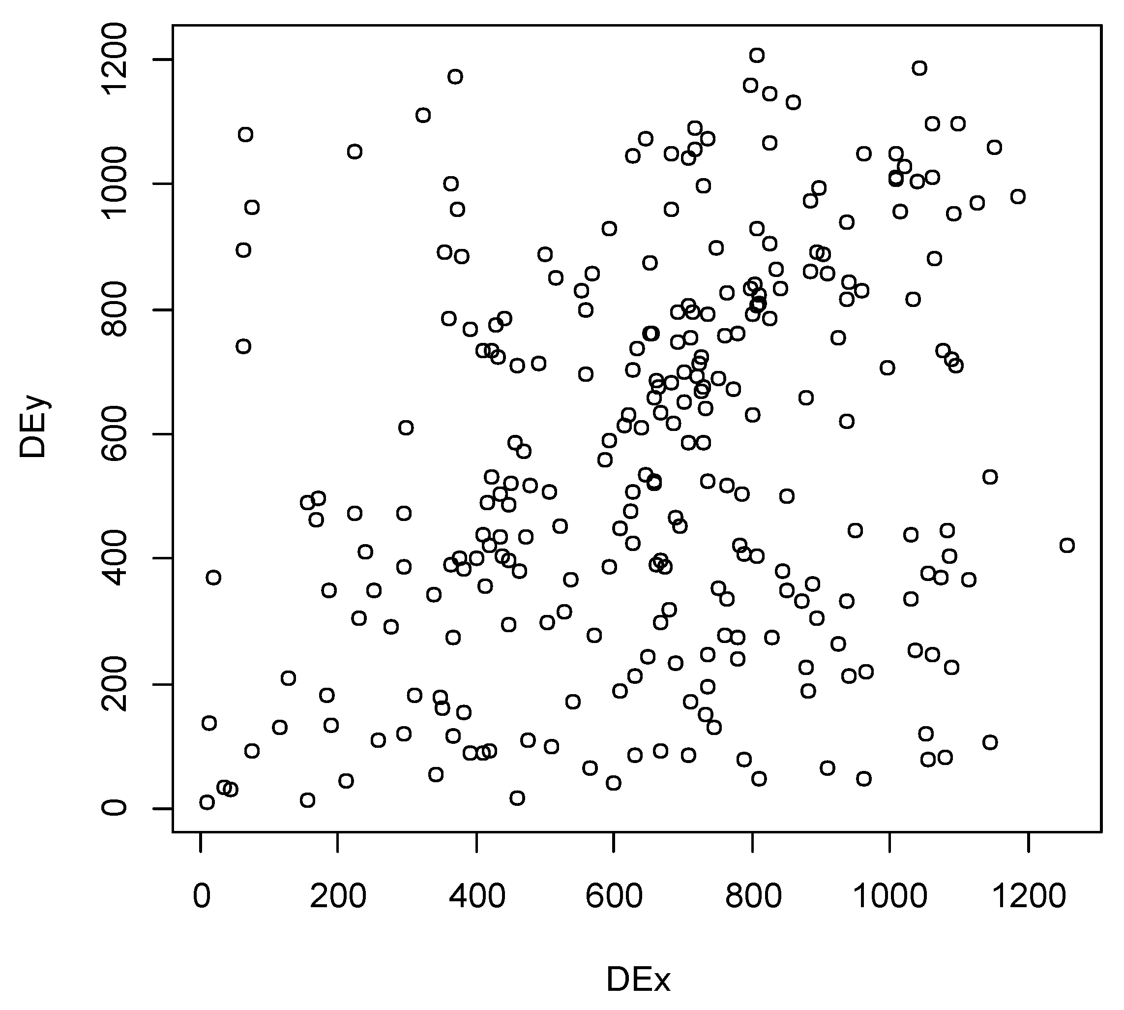
The scatterplot in Figure 2 shows the correlation between failures of the crankshaft position sensor (D) and oxygen heated sensor (E). While these components demonstrated the lowest association out of all ten pairs considered, they still exhibited some positive correlation. These two extreme examples of high and low association between failure times illustrated the variety of patterns we were trying to model.

3. Copula Models of Dependence

Since failures in all ten pairs can be related, we built a model of the joint distribution that captured the probabilities of two components failing before specific dates. Copulas are special binary functions making it possible to model the joint distribution of several random variables by separately modeling the marginal distributions of the variables and their dependence structure. We restricted our attention to pair copulas. Let X and Y be two random variables with respective c.d.f.s $u=F\left(x\right)$ and $v=G\left(x\right)$. Then, we represent their joint distribution $P(X\le x,Y\le y)$, or joint survival function $P(X>x,Y>y)$, as $C\left(F\right(x)$, $G\left(y\right)\left|\alpha \right)=C(u,v|\alpha )$, where u and v are marginal distributions, C is a copula function from a certain class, and $\alpha$ is the association parameter measuring the strength of dependence. We will consider the following four one-parametric families of copulas, for which there exist simple relationships between the association parameter and Kendall’s concordance $\tau$ defined in (Kendall 1938). Kendall’s $\tau$ is widely used as a non-parametric measure of association in statistical dependence studies, as a distribution-free alternative to Pearson’s correlation. We will express all four copula models in terms of Kendall’s concordance as $C(u,v|\tau )=C(u,v\left|\tau \right(\alpha \left)\right)$.

3.1. Types of Copulas

Hypothesis 1 (H1).

Clayton’s copula:

$$P(X\le x,Y\le y)=C_1(u,v|\tau )=max\left\{{(u^{\frac{2\tau }{\tau -1}}+v^{\frac{2\tau }{\tau -1}}-1)}^{\frac{\tau -1}{2\tau }},0\right\},-1<\tau <1;$$

Hypothesis 2 (H2).

Gumbel–Hougaard’s copula:

$$P(X\le x,Y\le y)=C_2(u,v|\tau )=exp\left\{-{\left[{(-lnu)}^{\frac{1}{1-\tau }}+{(-lnv)}^{\frac{1}{1-\tau }}\right]}^{1-\tau }\right\},0\le \tau <1;$$

Hypothesis 3 (H3).

The dual (survival) Clayton’s copula:

$$P(X>x,Y>y)=C_3(1-u,1-v|\tau )=1-u-v+C_1(u,v|\tau ).$$

Hypothesis 4 (H4).

The dual (survival) Gumbel–Hougaard’s copula:

$$P(X>x,Y>y)=C_4(1-u,1-v|\tau )=1-u-v+C_2(u,v|\tau ).$$

The relationship between $\alpha$ and $\tau$ for the models H1 and H3 is $\tau =\alpha /(\alpha +2)$, and for the models H2 and H4, $\tau =1-1/\alpha$.

These four families represent the most popular one-parametric Archimedean copulas, widely used in survival analysis and known to model effectively dependence in the tails of the joint distribution (bivariate extremes). They are also convenient because, as we can see, there exists a direct relationship between the parameters of association $\alpha$ (in all four cases, they have different meanings and different ranges) and Kendall’s $\tau$, which in all four cases is the same universal measure of association and can be compared between the models.

3.2. Tail Dependence

Tail dependence describes extreme comovements of a pair of random variables in the tails of the distributions. The definitions of tail dependence coefficients for copulas $C(u,v)$ with marginals $u=F\left(x\right)$ and $v=G\left(y\right)$ are as follows:

Lower tail dependence coefficient:

$${\lambda }_l=\underset{q\to 0^{+}}{lim}P(F\left(X\right)\le q|G\left(Y\right)\le q)=\underset{q\to 0^{+}}{lim}\frac{C(q,q)}{q}.$$

Upper tail dependence coefficient:

$${\lambda }_u=\underset{q\to 1^{-}}{lim}P(F\left(X\right)>q)|G\left(Y\right)>q)=\underset{q\to 1^{-}}{lim}\frac{1-2q+C(q,q)}{1-q}.$$

Certain copulas, such as the Gaussian copula, do not allow for tail dependence (their tail dependence coefficients are equal to zero). Some copulas (e.g., H1–H4) exhibit only either upper or lower tail dependence, while the t-copula and BB1 family (Joe 1997) are characterized by both lower and upper tails. Thus, when selecting an accurate copula model for specific data, it is important to consider whether the data display upper and/or lower tail dependence. In our case, lower tails (Models H1 and H4) corresponded to early failures of two engine subassembly components during the warranty period, which could reflect some early detected defects. Upper tails (Models H2 and H3) corresponded to relatively long lives of two components during the warranty period. Upper tail events were of interest since they represented failures late in the warranty period, which should be avoided from the manufacturer’s point of view. One of the problems with right censoring of the data corresponded to a possible misrepresentation of the right tails. The following formulas could be used to calculate the lower and/or upper tail dependences of the four selected copula models: H1: ${\lambda }_l=2^{\frac{\tau -1}{2\tau }}$, H2: ${\lambda }_u=2-2^{1-\tau }$, H3: ${\lambda }_u=2^{\frac{\tau -1}{2\tau }}$, and H4: ${\lambda }_l=2-2^{1-\tau }$.

4. Estimation of Copula Parameters

For a matched i.i.d. sample $(x_i,y_i),i=1,\dots ,n,$ we used copulas to model the joint distribution of the underlying variables X and Y. We used a two-step approach also known as IFM (inference from the margins) (Joe 1997). First, estimate the marginal distributions of X and Y as $\widehat{u}=\widehat{F}\left(x\right)$ and $\widehat{v}=\widehat{F}\left(y\right)$ to obtain the sample $D=\widehat{u_i},\widehat{v_i},i=1,\dots ,n$, and then, estimate the association parameter $\alpha$ for the copula $C(\widehat{u},\widehat{v}\mid \alpha )$. It is possible to use a sensible parametric model for marginals and then estimate the association. The properties of the estimates obtained by this approach were fully investigated in (Joe 1997) and (Joe 2014). The Weibull distribution often provides a good fit for individual parts’ TTFs. In this paper, we aimed to use a fully parametric approach carried out in two stages: First, estimate the TTF distribution for individual failures of Components A-E using the Weibull model. Here, we will use the results of (Baik 2010; Wu et al. 2000). Then, we estimated the parameter of association expressed through Kendall’s concordance using the estimates of the marginals $\widehat{u}$ and $\widehat{v}$. In this paper, we concentrated on the second step. An alternative approach suggesting non-parametric estimation of the margins was introduced and justified by (Genest and Rivest 1993) and followed by many other authors including (Shemyakin and Kniazev 2017).

Notice that another approach suggesting one-step estimation of all parameters of a pair copula (both association and marginal parameters)wasis less logical when we considered multiple pair copulas sharing the same components, because in this case, the analysis of different pair copulas may lead to different parametric estimates for one component’s marginal distribution.

For each of the four classes, we can define copula density as:

$$c_k(u,v|\tau )=\frac{{\partial }^2{C}_k(u,v|\tau )}{\partial u\partial v},k=1,\dots ,5.$$

4.1. Right Censoring (I)

The right censoring approach (I) as described in (Shih and Louis 1995) can be applied for every pair of components $(X,Y)$ to the entire sample of cars $(x_i,y_i),i=1,\dots ,n=32,667,$ where if a failure is not recorded for the first and/or the second component, $x_i$ and/or $y_i$ are set at the censoring values $T_i$ corresponding to the time from sale to the end of the observation or the warranty period (whichever comes first). If we denote ${\delta }_{xi}=I\{x_i<T_i\}$ and ${\delta }_{yi}=I\{y_i<T_i\}$ and use parametric estimates $\widehat{u}=\widehat{F}\left(x\right)$ and $\widehat{v}=\widehat{F}\left(y\right)$, the pseudolikelihood function can be represented as:

$$L_k\left(D\right|\tau )=\prod _{i=1}^n{c}_k{(\widehat{u_i},\widehat{v_i}|\tau )}^{{\delta }_{xi}{\delta }_{yi}}{\frac{\partial C_k(u,\widehat{v_i}|\tau )}{\partial u}{|}_{u=\widehat{u_i}}}^{{\delta }_{xi}(1-{\delta }_{yi})}\times$$

$$\times {\frac{\partial C_k(\widehat{u_i},v|\tau )}{\partial v}{|}_{v=\widehat{v_i}}}^{(1-{\delta }_{xi}){\delta }_{yi}}{C}_k{(\widehat{u_i},\widehat{v_i}|\tau )}^{(1-{\delta }_{xi})(1-{\delta }_{yi})}.$$

Using numerical implementation of the unweighted maximum likelihood method (Emura et al. 2010), we obtain an estimate $\widehat{\tau }$ for the model H1 along with the estimates of the parameters of the marginal distributions. We present these values for the model H1 for each of the ten pairs of five components in

Table 2. Estimates of association with right censoring.

	H1 $\widehat{\mathit{\alpha }}$	H1 $\widehat{\mathit{\tau }}$
AB	2.64	0.57
AC	−0.05	−0.03
AD	−0.20	−0.33
AE	−0.57	−0.40
BC	−0.27	−0.16
BD	0.16	0.08
BE	−0.51	−0.34
CD	−0.41	−0.25
CE	−0.59	−0.42
DE	−0.61	−044

.

This result demonstrated several problems with the right censoring approach (I). First, the values of $\widehat{\tau }$ appeared to be both positive and negative, though this was counterintuitive, and we expected mostly positive correlations between the failure times. This would create issues for the models H2 and H4, which allowed for only positive association. Second, the Weibull parametric model with such a heavy censoring became unrealistic and unreliable, hardly passing the goodness-of-fit test suggested in (Emura et al. 2010). It was possible that a mixture of Weibull distributions (Razali and Al-Wakeel 2013) could be a better fit. Finally, our goal of studying both tails of the warranty period (related failures occurring either early and or late) was not achieved by consideration of right censoring (I). Therefore, for the paired copula study, we concentrated on the conditional approach (II).

4.2. Conditioning to Failures in the Warranty Period (II)

If according to Approach (II), we considered for each pair of components only the subsamples where both failures occurred during the warranty period, the pseudolikelihood function for the copula estimation can be written as:

$$L_k\left(D\right|\tau )=\prod _{i=1}^n{c}_k{(\widehat{u_i},\widehat{v_i}|\tau )}^{{\delta }_{xi}{\delta }_{yi}}=\prod _{i=1}^{m_{XY}}{c}_k(\widehat{u_i},\widehat{v_i}|\tau ),$$

where $m_{XY}$ are the sample sizes from Table 1.

The Weibull distribution was assumed for all five marginals and demonstrated a plausible goodness-of-fit as illustrated in

Table 3. Estimates of marginal parameters.

	Shape	Scale
A	1.25	393
	(0.02)	(6.4)
B	1.52	521
	(0.03)	(8.2)
C	1.09	351
	(0.01)	(4.4)
D	1.92	643
	(0.03)	(7.1)
E	1.35	480
	(0.01)	(4.1)

.

Bayesian estimates of $\tau$ for Approach (II) were calculated under the assumption of a uniform prior on $\tau \in (0,1)$. The posterior estimate was obtained via the standard random walk Metropolis algorithm. The independent Metropolis algorithm with a uniform proposal also provided consistent conclusions. Numerical results (parametric estimates with standard errors in parentheses) are presented in

Table 4. Estimates of association conditioned to two failures (good matches indicated by asterisks).

	H1 $\widehat{\mathit{\tau }}$	H2 $\widehat{\mathit{\tau }}$	H3 $\widehat{\mathit{\tau }}$	H4 $\widehat{\mathit{\tau }}$	Sample $\mathit{\tau }$	Sample Size
AB	0.43	0.63	0.58	0.56	0.707	467
	(0.02)	(0.01)	(0.02)	(0.02)
AC	0.12	0.28*	0.28 *	0.14	0.269	441
	(0.02)	(0.01)	(0.03)	(0.02)
AD	0.20	0.36 *	0.32 *	0.26	0.375	152
	(0.03)	(0.04)	(0.04)	(0.04)
AE	0.12	0.24	0.22	0.12	0.314	307
	(0.01)	(0.03)	(0.03)	(0.02)
BC	0.16	0.32 *	0.28 *	0.20	0.307	260
	(0.03)	(0.03)	(0.03)	(0.04)
BD	0.24	0.40 *	0.36 *	0.33 *	0.400	160
	(0.04)	(0.04)	(0.04)	(0.04)
BE	0.12	0.33 *	0.32	0.15	0.386	258
	(0.02)	(0.03)	(0.03)	(0.03)
CD	0.12	0.31	0.32	0.15	0.452	271
	(0.02)	(0.03)	(0.03)	(0.03)
CE	0.17	0.30 *	0.28	0.23	0.318	686
	(0.02)	(0.02)	(0.02)	(0.02)
DE	0.18 *	0.27	0.25	0.23 *	0.188	267
	(0.03)	(0.04)	(0.03)	(0.04)

, while some posterior characteristics are illustrated in Figure 3 and Figure 4. Values with an asterisk are Bayes estimates falling within two standard errors from the sample concordance, indicating successful representation of data concordance by the corresponding copula model.

5. Comparison of Copula Classes

It was hard to suggest a clear choice between the models based on the results in Table 4; however, one could make an intuitive conclusion that when the estimated (model-induced) value of $\tau$ corresponding to the model Hi was close to the sample concordance, it indicated that the model Hi captured most of the association contained in the paired data. Models H1 and H4 were characterized by the lower tail dependence, while H2 and H3 were distinguished by upper tail dependence. Therefore, it was reasonable to believe that H1 and H4 appeared more adequate than H2 and H3 in the presence of lower tail dependence in the data and vice versa. This approach is further illustrated in

Table 5. Tail dependence induced by the model with conditioning to two failures.

	H1 (Lower)	H2 (Upper)	H3 (Upper)	H4 (Lower)
AB	0.63	0.71	0.77	0.65
	(0.03)	(0.02)	(0.01)	(0.03)
AC	0.07	0.35	0.40	0.19
	(0.03)	(0.09)	(0.05)	(0.15)
AD	0.26	0.44	0.47	0.33
	(0.07)	(0.09)	(0.07)	(0.14)
AE	0.07	0.30	0.29	0.16
	(0.02)	(0.11)	(0.06)	(0.14)
BC	0.16	0.39	0.42	0.26
	(0.06)	(0.09)	(0.06)	(0.17)
BD	0.33	0.48	0.54	0.41
	(0.08)	(0.09)	(0.05)	(0.13)
BE	0.08	0.41	0.47	0.19
	(0.04)	(0.07)	(0.05)	(0.16)
CD	0.07	0.38	0.47	0.20
	(0.04)	(0.09)	(0.04)	(0.20)
CE	0.19	0.38	0.41	0.29
	(0.04)	(0.06)	(0.04)	(0.08)
DE	0.21	0.14	0.35	0.28
	(0.07)	(0.04)	(0.06)	(0.14)

by the tail dependence values calculated using the concordance estimates in Table 5 with the propagation of errors.

5.1. Tail Dependence

It looks from Table 5 like upper tail dependence was more pronounced in the data for nine pairs excluding DE. This could be illustrated by Figure 1 and Figure 2 and also by the analysis of the failures of Components B (ignition coil assembly) and E (oxygen heating sensor), where this effect was especially strong. It happened that one of these components failed early, and the other failed in the middle of the warranty period, while at the end of the warranty period, both tended to fail simultaneously or directly one after the other. This suggested the choice of the model H2 (Gumbel–Hougaard) or H3 (survival version of Clayton) since they attributed the association in paired data to upper tail dependence.

5.2. Information Criteria

To determine which of the four copula classes H1–H4 provided the best fit, one could consider conventional likelihood based tools. One of the ways to compare non-nested models involves information criteria. Applying the Akaike information criterion (AIC) and Bayes information criterion (BIC) as shown in (Shemyakin and Kniazev 2017) demonstrated that the two-parameter classes of Archimedean BB1 copula and Student t-copula provided a better fit than the one-parameter Archimedean copulas. However, the classes H1-H4 also demonstrated a relatively good fit.

5.3. Kolmogorov–Smirnov Statistic

The Kolmogorov–Smirnov distance measures the maximum distance between a cumulative distribution function (c.d.f.) and its empirical cumulative distribution function (e.c.d.f.). For a given c.d.f. $F\left(x\right)$ and e.c.d.f. $F_n\left(x\right)$, the Kolmogorov–Smirnov distance can be computed as follows:

$$D_n=\sqrt{n}\underset{x}{sup}|F_n\left(x\right)-F\left(x\right)|.$$

It is also applicable to the multivariate case, though its calculation is less straightforward, and its use for goodness-of-fit testing is more complicated. the Kolmogorov–Smirnov statistic in multiple dimensions is no longer distribution-free, and the most practical way to assess its critical values involves a Monte Carlo simulation (Justel et al. 1997).

All of these criteria (AIC, BIC, or KS statistic) of finding the best class of pair copula models share the same issue: the entire analysis is restricted to the comparison of single representatives of each class obtained by point estimation; thus, the results are subject to its accuracy. The following section discusses one possibility to make choices among H1-H4 based on multiple representatives of these classes.

6. Bayesian Model Selection

In order to compare four different families of copulas in a parametric setup, we had to determine a universal parameter, which could be evaluated for each of the families. A natural choice is to use Kendall’s concordance $\tau$ as the universal parameter. Sample concordance $\widehat{\tau }$ is a reasonable non-parametric estimator of $\tau$ (Kendall 1938). The proximity of the model induced estimates of $\tau$ in Table 3 may serve as a measure of model performance. However, this comparison still relied on single point estimates to represent entire families.

Following (Bretthorst 1996; Huard et al. 2006; Shemyakin and Kniazev 2017), we compared the data fit provided by thew models H1-H4 not at a single value of the association parameter(s) obtained by MPLE, but rather over the set of possible association values selected from a reasonable range. This could be accomplished by specifying a prior distribution for association parameter(s) and integrating the likelihood with respect to the prior distribution. The problem is the difference of meaning and ranges of association parameters for different copula classes. However, this problem is resolved by specifying a prior on universal parameter $\tau$.

We will assume that the four classes H1–H4 represent exhaustive and mutually exclusive hypotheses. The posterior probabilities of these hypotheses may be rewritten as:

$$P(H_k\mid D)=\int P(H_k,\tau \mid D)d\tau =\frac{\int P(D\mid H_k,\tau )P(H_k\mid \tau )\pi \left(\tau \right)d\tau }{P\left(D\right)},$$

(1)

where we will consider all four hypotheses a priori equally likely, the dependence between variables being positive, which suggests $\tau \ge 0$. In this case, the natural choice of the prior for $\tau$ is the Beta distribution. The choice of parameters for the prior may be suggested by sample concordance for the entire dataset consistent with the empirical Bayes approach: $P(D\mid H_k,\tau )=L_k(D\mid \alpha \left(\tau \right)),P(H_k\mid \tau )=P\left(H_k\right)=\frac{1}{4},\pi \left(\tau \right)\sim Beta(\widehat{a},\widehat{b})$. However, a good starting choice in this context may be the uniform prior $Beta(1,1)$.

We will not need to calculate the denominator of the posterior in (1). It suffices to calculate the weights:

$$W_k={\int }_0^1{L}_k(D\mid \tau )\pi \left(\tau \right)d\tau ={\int }_0^1{\Pi }_{i=1}^n{c}_k({\widehat{u}}_i,{\widehat{v}}_i\mid \tau )\pi \left(\tau \right)d\tau ,k=1,2,3,4,$$

(2)

or using the Monte-Carlo approach and drawing samples from the Beta prior, evaluate:

$${\widehat{W}}_k=\frac{1}{N}\sum _{j=1}^N{\Pi }_{i=1}^n{c}_k({\widehat{u}}_i,{\widehat{v}}_i\mid {\tau }_j).$$

(3)

Table 6. Posterior probabilities for H1–H4, highest row values boldfaced.

	H1	H2	H3	H4
AB	0	1	0	0
AC	0	0.996	0.004	0
AD	0	0.995	0.001	0.004
AE	0	0.997	0	0.003
BC	0	0.999	0.0005	0.0005
BD	0	0.989	0.010	0.001
BE	0	1	0	0
CD	0	0.136	0.864	0
CE	0	1	0	0
DE	0.001	0.983	0.009	0.007

contains the estimates of the posterior probabilities of Hypotheses H1–H4 based on ${\widehat{W}}_k$:

$$\widehat{P}\left(H_k\right|D)=\frac{{\widehat{W}}_k}{{\sum }_{j=1}^4{\widehat{W}}_j},$$

(4)

calculated by $N=$ 10,000 runs of direct Monte Carlo sampling from the uniform prior. The highest values for each pair of components are boldfaced.

From Table 6, we can see that upper tail copulas H2 (and to a certain extent, H3) had much higher posterior probabilities. Out of these two, the Gumbel–Hougaard copula H2 nine out of ten times had much higher posteriors than the Clayton survival model H3. This conclusion was based on the integration of the likelihood over a range of values of concordance and was therefore more reliable than a comparison based on estimated posterior means for different models in Table 4 or Table 5. The use of a flat prior allowed us to concentrate on the properties of likelihood without much sensitivity to the point estimation of association parameters.

7. Higher Dimensions

One may consider the possibility of building higher dimensional models for our choice of five components. For Archimedean copulas H1–H4, it is a non-trivial task, since dimensions higher than two require additional determination of the hierarchical structure. The most popular multidimensional Archimedean copulas are based on pair-copula constructions such as vines (Aas et al. 2009) or nested copulas (Hofert and Maechler 2011). However, for elliptical copulas (including Student’s t-copula), a simple generalization to higher dimensions is straightforward using the package described in (Kojadinovic and Yan 2010). Various generalizations of Student copulas allowing for the lack of symmetry of two tails and the individual number of degrees of freedom for each component were discussed, for instance, in (Demarta and McNeil 2005; Yoshiba 2018).

Unfortunately, the occurrences of three or more component failures during the warranty period were relatively rare in our database: 25 cases for A, B, and D and just one for all five components. Conditioning (II) cannot bring about reliable results due a small sample size. Some of the results of applying the right censoring scheme (I) with the five-dimensional symmetric t-copula based on 32,667 observations using the software of (Kojadinovic and Yan 2010) are provided in

Table 7. Parametric estimates for t-copula, 5 dimensions.

Parameter	Estimate	St.error	z-value	Pr(>|z|)
correlation (AB)	0.8015	0.0019	430.2	$<2\times {10}^{-16}$
correlation (AC)	0.8073	0.0016	506.5	$<2\times {10}^{-16}$
correlation (AD)	0.7609	0.0028	276.2	$<2\times {10}^{-16}$
correlation (AE)	0.7241	0.0034	212.8	$<2\times {10}^{-16}$
degrees of freedom	1.9329	NA	NA	NA

: point estimates along with standard errors, z-scores, and the p-values of the z-test.

Two apparent problems with the estimates in Table 7 were: higher pairwise correlations (compare to Table 4) and the low number of degrees of freedom, which did not allow analyzing the estimation errors. Both of these issues may be due to heavy right censoring caused by a low count of critical events in higher dimensions.

8. Conclusions

The warranty claim data analyzed in (Kumerow et al. 2014; Shemyakin and Kniazev 2017) and the current paper demonstrated a substantial dependence observed between the TTFs for automotive components related to the engine subassembly of Hyundai Accent vehicles. This dependence addressed simultaneous failures, as well as consecutive failures of different components within the warranty period, with the latter being especially important for predictive analysis, suggesting an increased probability of a component after a repair or replacement of another component. The assumption of independence would lead to grossly underestimated related failure risks and warranty costs.

This dependence can be related to multiple causes, including:

• simultaneous failure as a result of one critical event;
• similar exploitation and maintenance patterns;
• wear and tear of engine components due to other components’ malfunction;

roughly corresponding to common disaster, common lifestyle, and broken-heart syndrome, as pertaining to life insurance.

These multiple causes of failures can be addressed using pair copula models. Open source software packages in the R environment (Brechmann and Schepsmeier 2013; Kojadinovic and Yan 2010) allow for a straightforward implementation of parametric and semi-parametric estimation for different classes of copulas including those discussed in the paper: direct and dual Archimedean copulas (Clayton and Gumbel–Hougaard classes).

Dealing with the incomplete data confined to the warranty period presented a challenge. Using standard right censoring techniques as in (Schemper et al. 2013) and Approach (I) of the current paper did not properly address tail dependence, especially events at the end of the warranty period. On the other hand, Approach (II) introduced in (Kumerow et al. 2014) and used in (Shemyakin and Kniazev 2017) restricted the sample sizes and thus limited the scope of high-dimensional analysis.

The problem of model selection, including an adequate choice of copula, plays a special role, since the model probabilities of failure substantially depend on the copula type. For model comparison, one can consider tail dependence, information criteria, or the Kolmogorov–Smirnov statistic as a good measure of overall fit; see also (Shemyakin and Kniazev 2017). However, one may prefer Bayesian model selection between classes of copulas using Kendall’s tau as the common parameter for different classes of copulas (Huard et al. 2006). This approach to model selection allows for a comparison of copula families based on multiple representatives of each class; therefore, it is less sensitive to methods of point estimation within different classes.

We restricted ourselves to four one-parameter one-tailed Archimedean copulas in order to illustrate the relationship between the tail dependence and model selection. The results of the Bayesian procedure summarized in Table 6 suggested that the upper tail dependence (events at the end of the warranty period) played a special role in modeling related failures. However, we have to notice that for TTFs of engine subassembly components, most of the tools of model selection indicated t-copulas being superior to the four considered Archimedean copulas. This fact could be explained by the t-copulas exhibiting tail dependence in the both lower and upper tails of the joint TTF distribution, while Archimedean copulas H1-H4 concentrated at one of the tails. However, it was not clear whether the assumption of the symmetry of the tails of t-copulas was plausible and not too restrictive. One possible suggestion for future work is to use more complex hybrid or mixed Archimedean copula models as an alternative to t-copulas; see also (Komornikova and Komornik 2010). An alternative approach involves skewed or asymmetric t-copulas or other more complex extensions of elliptical copula models, as suggested in (Yoshiba 2018).