Article

Bankruptcy Prediction and Stress Quantification Using Support Vector Machine: Evidence from Indian Banks

by
Santosh Kumar Shrivastav
* and
P. Janaki Ramudu
Institute of Management Technology, Nagpur 441502, India
*
Author to whom correspondence should be addressed.
Risks 2020, 8(2), 52; https://doi.org/10.3390/risks8020052
Submission received: 25 February 2020 / Revised: 22 April 2020 / Accepted: 21 May 2020 / Published: 22 May 2020
(This article belongs to the Special Issue Credit Risk Modeling and Management in Banking Business)

Abstract

:
Banks play a vital role in strengthening the financial system of a country; hence, their survival is decisive for the stability of national economies. Therefore, analyzing the survival probability of the banks is an essential and continuing research activity. However, the current literature available indicates that research is currently limited on banks’ stress quantification in countries like India where there have been fewer failed banks. The literature also indicates a lack of scientific and quantitative approaches that can be used to predict bank survival and failure probabilities. Against this backdrop, the present study attempts to establish a bankruptcy prediction model using a machine learning approach and to compute and compare the financial stress that the banks face. The study uses the data of failed and surviving private and public sector banks in India for the period January 2000 through December 2017. The explanatory features of bank failure are chosen by using a two-step feature selection technique. First, a relief algorithm is used for primary screening of useful features, and in the second step, important features are fed into the support vector machine to create a forecasting model. The threshold values of the features for the decision boundary which separates failed banks from survival banks are calculated using the decision boundary of the support vector machine with a linear kernel. The results reveal, inter alia, that support vector machine with linear kernel shows 92.86% forecasting accuracy, while a support vector machine with radial basis function kernel shows 71.43% accuracy. The study helps to carry out comparative analyses of financial stress of the banks and has significant implications for their decisions of various stakeholders such as shareholders, management of the banks, analysts, and policymakers.

1. Introduction

Indian banks are strongly capitalized, well-regulated, and have been monitored by the Reserve Bank of India (RBI) for over a decade. The banking sector is highly interconnected with daily economic activity, and any major failures in the sector pose operational and financial risks. Due to these possible risks, the RBI has tried to maintain the financial stability of banks by providing appropriate monetary policy support from time to time. The financial disaster during 2007–2008 is one example that spread internationally over time. The RBI has taken certain important steps to ensure the financial stability of Indian banks, such as Prompt Corrective Action (PCA) and capital infusion. It has also provided a recapitalization package for public sector banks in October 2017 to the tune of Rs. 2.11 trillion.
The high probability of similar financial crises in the future warrants the need for close and strict supervision of the banks and an appropriate action plan. Bankruptcy prediction is crucial, and developing a technique to measure financial distress before it actually occurs is important. As a result, formulating precise and efficient bankruptcy prediction models have become important. The financial institutions are concentrating on developing an understanding of their drivers of success, which include better uses of its resources like technology, infrastructure, human capital, the process of delivering quality service to its customers, and performance benchmarking. Performance analyses of current financial institutions use traditional techniques like finance and accounting ratios, debt-to-equity proportions, returns on equity, and returns on assets, but these methods all have methodological limitations (Yeh 1996).
There is a significant amount of literature that deals with bankruptcy prediction using statistical techniques (Altman 1968; Meyer and Pifer 1970; Altman et al. 1977; Martin 1977; Ohlson 1980; Zmijewski et al. 1984; Whalen 1991; Cole and Gunther 1998; Shumway 2001; Cole and Gunther 1995; Lin et al. 2011 and many more). Several recent studies have been conducted for bankruptcy prediction using machine learning techniques as well (Lin et al. 2011; Antunes et al. 2017; Kirkos 2015; Murphy 2012; Shrivastava et al. 2020). Most machine learning techniques find common patterns in failed banks based on financial and nonfinancial information.
An innovative bankruptcy predictive model and a stress quantification technique are developed in this study using a support vector machine (SVM) with suitable kernels for Indian banks. In this new approach, first the instance-based method “Relief Algorithm” was used for the initial screening of feature selection, which is a nonparametric method. Many previous researchers have used parametric methods for feature selection, as discussed in the literature. Second, we developed a SVM model and tuned the parameter using 5-fold cross-validation, which helps in the generalization of the model by developing an optimal cut-off level, while many previous researchers used the default cut-off level. Third, geometric analysis of the proposed machine learning technique in this study is beneficial for stress quantification and provides a tool to regulators for tracking and comparing different banks’ financial status. This is the first study of its kind on Indian banks where stress quantification is derived using SVM.
The paper is organized as follows: Section 1 contains an introduction; Section 2 contains a literature review; Section 3 contains methodology and data descriptions; Section 4 explains empirical results, findings, and stress quantification; Section 5 contains the conclusions of the study; and Section 6 explains the limitations of the study.

2. Literature Review

Practitioners and academicians are currently using artificial intelligence (AI) and machine learning (ML) approaches to predict bankruptcy. For instance, Tam (1991) used a back-propagation neural network (BPNN) to conduct bankruptcy prediction for US banks, and the input features were selected based on capital adequacy, asset quality, management quality, earnings, and liquidity (CAMEL) metrics. Tam concluded that the BPNN gives better predictive accuracy than other techniques like discriminant analysis (DA), logistic regression (LR), and K-nearest neighbor (K-NN). Also, Sharda and Wilson (1993) compared the usefulness of BPNN with multi-discriminant analysis (MDA) for bankruptcy prediction and found that the BPNN’s performance was better than that of MDA in all scenarios. Fletcher and Goss (1993) used the BPNN with 5-fold cross-validation for bankruptcy prediction and equated its results with the ones obtained from logistic regression (LR) using data collected for 36 companies. The authors found that BPNN had 82.4% prediction accuracy compared to the 77% from logistic regression.
Altman et al. (1994) compared the accuracy of linear discriminant analysis (LDA) with BPNN in distress classification using financial ratios and found that LDA performed better than BPNN. Tsukuda and Baba (1994) formulated a predictive model for bankruptcy using BPNN with one hidden layer and found that BPNN had better accuracy than discriminant analysis (DA). Cortes and Vapnik (1995) used SVM for the first time for two-group classification problems. Due to nonlinearly separable data, input factors were mapped to a very high-dimension feature space, the performance of the support vector machine was compared to various other machine learning algorithms. Leshno and Spector (1996) compared various neural network (NN) models with DA and described their prediction proficiencies in the form of data span, learning technique, convergence rate and number of iterations. Piramuthu et al. (1998) used a new set of features to improve the accuracy of the BPNN bankruptcy model for the dataset of 182 Belgium-based banks.
Swicegood and Clark (2001) used DA, BPNN, and human judgment to predict bank failure. They found that BPNN outperformed and provided the maximum accuracy when compared to the rest of the models. Neural network (NN) is perhaps the most significant forecasting tool to be applied to the financial markets in recent years and is gaining its prominence. Nanni and Lumini (2009) used the dataset of firms from countries like Australia, Germany, and Japan and found that machine learning techniques with bagging and boosting lead to better classification than standalone methods. Du Jardin (2012) found the significance of feature selection and its influence on the classification performance for the first time. The study revealed that NN gave better prediction accuracy when the input features were selected by definite criterion. Further, Wang et al. (2011) used ensemble methods with the base learners like logistic regression (LR), decision tree, artificial neural network (ANN) and SVM and found that the performance of bagging technique was better than the boosting technique for all the databases they analyzed. Chaudhuri and De (2011) used a novel approach known as a fuzzy support vector machine (FSVM) to solve bankruptcy classification problems. This extended model combines the advantages of both machine learning and fuzzy sets and equated the clustering power with a probabilistic neural network (PNN).
Tian et al. (2012) showed that machine learning techniques are the most important recent advances in applied and computational mathematics, which carry significant implications for classification problems. Chen et al. (2013) constructed a bankruptcy trajectory reflecting the dynamic changes of the financial situation of companies that enables them to keep track of the evolution of companies and recognize the important trajectory patterns. Korol (2013) investigated the effectiveness of statistical methods and artificial intelligence techniques for predicting the bankruptcy of enterprises in Latin America and Central Europe a year and two before bankruptcy and found that artificial intelligence techniques are more efficient in comparison to statistical techniques.
Wang et al. (2014) advocated that there is no mature or definite principle for a firm’s failure. Kim et al. (2015) proposed the geometric mean based boosting algorithm (GMBoost) to resolve the data imbalance problem for bankruptcy prediction. The authors applied GMBoost to bankruptcy prediction tasks to estimate its performance. The comparative analysis between GMBoost with AdaBoost and cost-sensitive boosting showed that GMBoost with AdaBoost is better than the cost-sensitive boosting in terms of high predictive power and robust learning capability in both imbalanced and balanced data. Papadimitriou et al. (2013) formulated the SVM bankruptcy predictive model using six input features on the dataset of 300 U.S. banks and achieved 76.40% of forecasting accuracy. Cleary and Hebb (2016) examined 323 failed banks and the same number of non-failed banks in the U.S. for the period 2002 through 2011. The author used DA and variables based on CAMEL to predict the failure of banks for unseen data and obtained 89.50% predictive accuracy.
Most of the previous research studies on bankruptcy prediction were focused on the country where the number of failed banks were large, but for a country like India, where the number of failed banks is less in comparison to the surviving banks, very few studies are available for bankruptcy prediction (Pramodh and Ravi 2007; Dash and Das 2009; Pradhan 2014; Shrivastava et al. 2020). Most studies have focused on creating a bankruptcy prediction model, and no one has attempted to calculate and compare the financial stress of Indian banks. In this research study, we derived a bankruptcy prediction model and developed a technique to calculate and compare the financial stress of Indian banks using SVM.

3. Data Descriptions and Methodology

Data were collected for failed and survived banks, public sector banks (public sector banks (PSBs) are a major type of bank in India, where a majority stake, i.e., more than 50%, is held by the government) and private banks (private sector banks in India are banks where the majority of the shares or equity are not held by the government but by private shareholders) in India for the period January 2000 to December 2017. In this research study, we assumed that a bank failed if any of these conditions occurred: merger or acquisition, bankruptcy, dissolution, and/or negative assets (Pappas et al. 2017; Shrivastava 2019). Data were collected for only those banks where data existed for four years before their failure. In the same way as the surviving banks, the last four years of data were considered in the sample. In our final sample, out of 59 banks, 42 banks were surviving banks and 17 were failed banks. For each bank, 25 features and financial ratios were calculated for four years (Pappas et al. 2017). In this way, in the sample, we had a total of 25 × 4 = 100 variables per bank (Pappas et al. 2017). The information about 25 features and financial ratios is given in Appendix A. During data collection, we treated data of the immediately preceding year (t−1) as recent and the data of (t−2), (t−3), and (t−4) as past information.
Data collected for the failed and survived banks for the period Jan. 2001 through Dec. 2017 contained a mix of importance and redundancy features. All features of the data collected for modeling are not equally important. Some have significant contributions, and some others have no significance in modeling. A model that contains redundant and noisy features may lead to the problem of overfitting. To reduce non-significant features and computation complexity in the forecasting model, well-known two-step feature selection techniques, relief algorithm and support vector machine, have been used.

3.1. Two-Step Feature Selection

In this study, we used the relief algorithm, an instance-based learning algorithm, which comes from the family of a filter-based feature selection technique (Kira and Rendell 1992; Aha et al. 1991). This algorithm maintains trade-off between the complexity and accuracy of any statistical or machine learning model by adjusting to various data features. In this feature selection method, the relief algorithm assigns the weight to explanatory features that measure the quality and relevance based on the target feature. This weight ranges between −1 and 1, where −1 shows the worst or most redundant features and +1 shows the best or most useful features. The relief algorithm is a non-parametric method that computes the importance of input features concerning other input features and does not make any assumptions regarding the distribution of features or sample size.
This algorithm just indicates the weight assigned to each explanatory feature but does not provide a subset of the features directly. Based on the output, we discarded all such features that had less than or equal to zero weight. The features having weights greater than zero will be relevant and explanatory. A computer pseudo-code for the feature selection relief algorithm is given below (Kira and Rendell 1992; Aha et al. 1991).
Initial Requirement: We need features for each instance where target classes are coded as −1 or 1 based on bankruptcy prediction. In this study, we used ‘R’ programming for the relief algorithm, where “M” denotes the number of records or instances selected in the training data, “F” denotes the number of features in each instance of training data, “N” denotes the random training instances from “M” instances of training data to update the weight of each feature, and “A” represents the randomly selected feature for randomly selected training instances.
The following is the pseudo-code for the relief algorithm (Kira and Rendell 1992; Aha et al. 1991):
Initially, we assume that the weight of each feature is zero, i.e., W [A]: = 0.0
For i: = 1 to N do
Select a random target instance say Li
Check the closest hit ‘H’ and closest miss ‘M’ for the randomly selected instance.
For A: = 1 to F do
Weight [A]: = Weight [A] − diff [A, Li, H]/N + diff [A, Li, M]/N
End for (second loop)
End for (First loop)
Return the weight of features.
The relief algorithm selects the instances from the training data say “Li” without replacement. For selected instances from training data, the weight of all features is updated based on the difference observed for target and neighbor instances. This is a cyclic process, and in each round the distance of the “target” instance with all other instances is computed. This method selects the two closest neighbor instances of the same class (−1 or 1) called the closest hit (‘H’) and the closest neighbor with a different class called the closest miss (‘M’). The weights are updated based on closest hit or closest miss. If it is the closest hit, or when the features are different for the same class of instances, the weight decreases by the amount 1/N, and when the features are different in the instances of a different class, the weight increases by the amount 1/N. This process continues until all features and instances are completed by the loop. The following is an example of the relief algorithm:
Class of Instances
Target Instance (Li) CDCDCDCDCDCDCD 1
Closest Hit (H)   CDCDCDCCCDCDCD 1
Risks 08 00052 i001
Here, due to mismatch between features in the instances of the same classes, indicated in the red color, a negative weight −1/N is allocated to the feature.
Class of Instances
Target Instance (Li) CDCDCDCDCDCDCD 1
Closest Hit (H)   CDCDCDCCCDCDCD −1
Risks 08 00052 i001
Here, due to mismatch between features in the instances of the different classes, indicated in red color, a positive weight 1/N is allocated to the feature. This process follows until the last instances and is valid for only discrete features.
The diff. function in the above pseudo-code computes the difference in the value of feature “A” with two instances I1 and I2, where I 1 = L i and I 2 is either “H” or “M” when performing weight updates. The diff. function for the discrete feature is defined as
  d i f f . ( A , I 1 , I 2 ) = { 0     i f     v a l u e ( A , I 1 ) = v a l u e ( A , I 2 ) 1       o t h e r w i s e  
and the diff. function for the continuous feature is defined as
d i f f . ( A , I 1 , I 2 ) = | v a l u e ( A , I 1 ) v a l u e ( A , I 2 ) | max ( A ) min ( A )    
The maximum and minimum values of feature “A” are calculated over all instances. Due to normalization of the diff. function, the weight updates for discrete and continuous features always lie between 0 and 1. While updating the weight of feature “A”, we divide the output of the diff. function by “N” to bring the final weights of features between 1 and −1. The weight of each feature calculated through the relief algorithm is listed in Appendix B. The selected features from the relief algorithm are fed into SVM to find the combination of significant features through an iterative process based on the target feature. The feature set that gives the highest accuracy of SVM is known as optimal features. There are several benefits of using a relief algorithm as an initial screening of features. First, the relief algorithm calculates the quality of the feature by comparing it with other features. Second, the relief algorithm does not require any assumptions on the features of the dataset. Third, it is a non-parametric method.
We used the R package “relief (formula, data, neighbours.count, sample.size)” to find the relief score as given in Appendix B, where argument “formula” is a symbolic description of the model, argument “data” is the data to process, argument “neighbours.count” is the number of neighbors to find for every sampled instance, and the argument “sample.size” is the number of instances to sample.

3.2. Support Vector Machine

3.2.1. Why Support Vector Machine?

Support vector machine is a machine learning algorithm established early in the 1990s as a nonlinear solution for the problem of classification and regression (Vapnik 1998). The basic idea behind the SVM model was to avoid the problem of overfitting, where most of the machine learning techniques suffer from this issue. SVM is an important and successful method because of many reasons. First, SVM is a robust technique and can handle a very large number of variables and small samples easily. Second, SVM employs sophisticated mathematical principles, for instance, K-fold cross-validation to avoid overfitting, and it gives better and superior empirical results over the other machine learning techniques. The third reason for using the support vector machine is an easy geometrical interpretation of the model when the data are linearly separable.

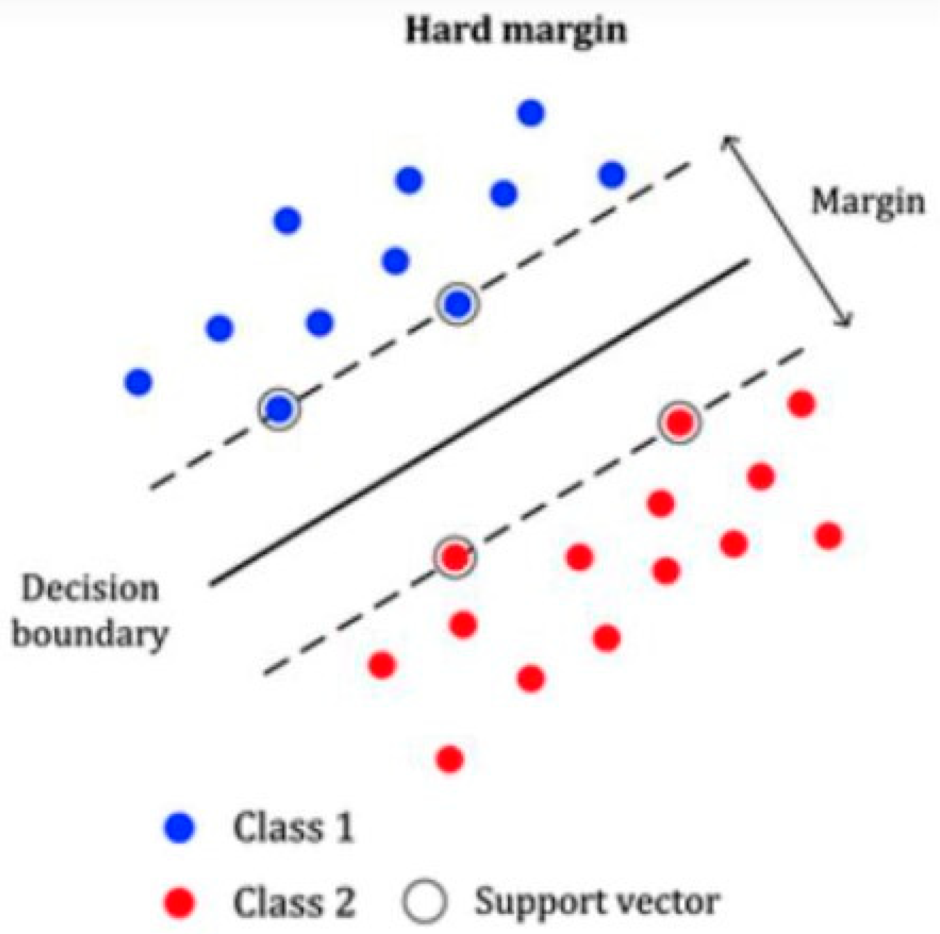
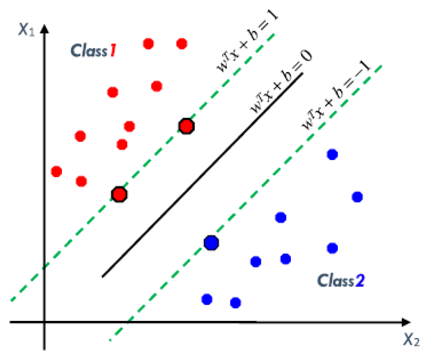
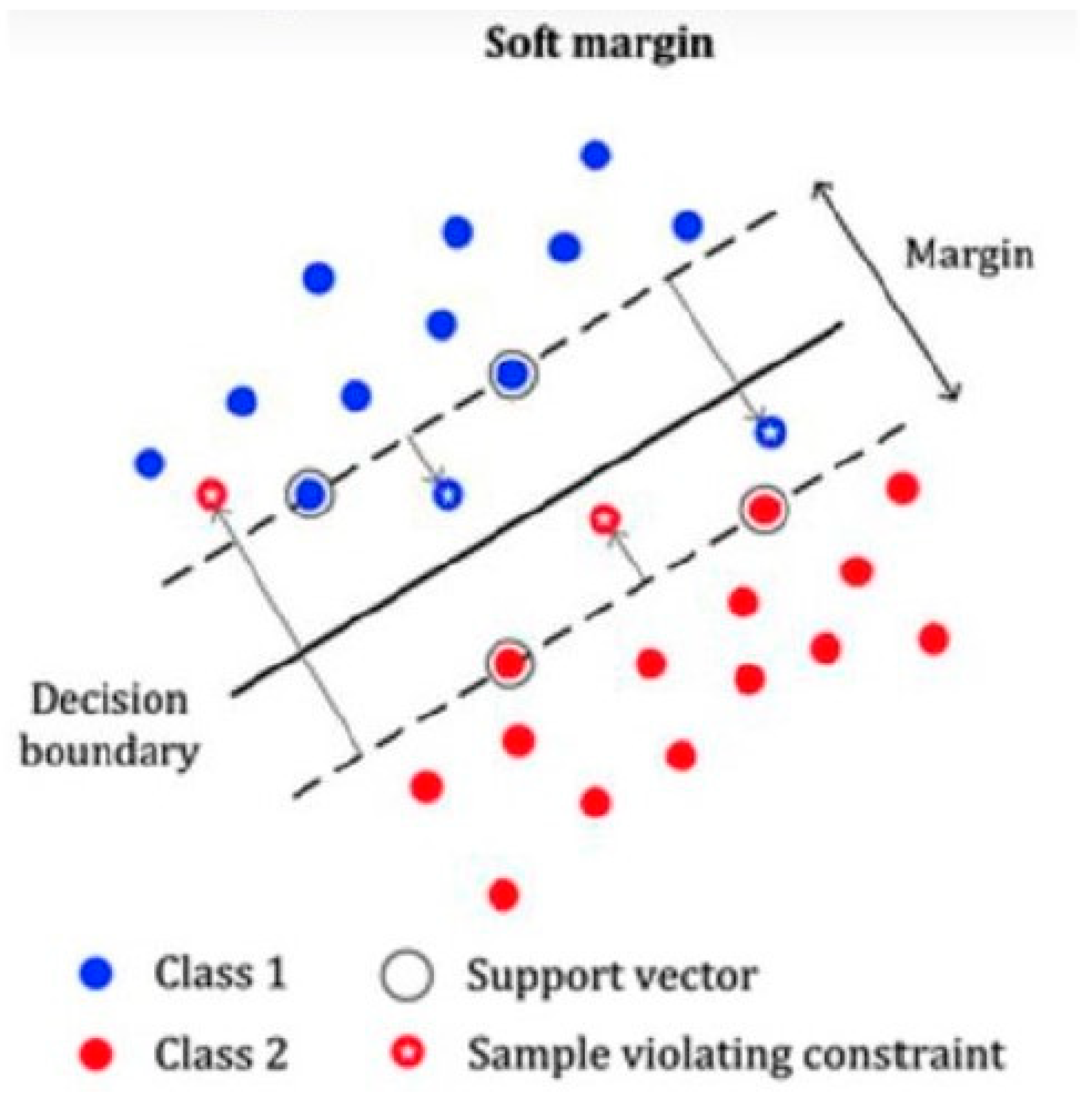
3.2.2. Support Vector Machine for Linearly Separable Data

SVM has been effectively applied in many areas to classify data into two or more than two classes (Vapnik 1998). The SVM finds a classification criterion that can separate data into two, or more than two, classes based on the target feature. If the data are linearly separable in two classes, then the classification boundary will be a linear hyperplane with a maximum distance from the data of each class. The mathematical equation of the linear hyperplane for training data z i ( i = 1 , 2 , 3 , , n ) is given as
w T z + b = 0
where w is an n-dimensional weight vector and b is the bias.
The hyperplane shown in Figure 1 separates data in two classes that must satisfy two conditions. First, the misclassification error should be at a minimum, and second, the distance of the linear hyperplane of the closest instance from each class should be at a maximum. Under the stated conditions, the instance of each class will be above or below the hyperplane. Two margins can, therefore, be defined as in Figure 2.
w T z + b { 1 f o r   y i = 1 1 f o r   y i = 1
Since the margin section for the decision boundary lies between [−1, +1], there is an infinite possible hyperplane that can be a decision boundary for each section, as shown in Figure 2. To get the optimal decision boundary, we need to maximize the distance “d” between the margins given as follows:
d ( w , b , z ) = | ( w T z + b 1 ) ( w T z + b + 1 ) | w = 2 w  
Maximizing the margin 2 w means minimizing   w   or 1 2 w T w . The modified optimization problem for the optimal decision boundary is given as follows:
M i n w , b = 1 2 w T w
s . t         y i ( w T z + b ) 1
We used the Lagrange multiplier (alpha) to find the combined Equations (4) and (5) as below:
L p ( w , b , α ) = 1 2 w T w i = 1 N α i { y i [ w T z i + b ] 1 }  
We determined the equation of the linear hyperplane by solving Equation (6) using the Karush–Kuhn–Tucker method (Mangasarian 1969).
There is always a likelihood that data are not easily linearly separable because of some similarities in input features of the dataset. Here, we used the modified SVM by introducing the concept of penalty. Figure 3 below represents the soft margin where data are not easily separable.
Let ξ be the distance between the wrongly classified data and the margin of that class. Then, the penalty function can be calculated as F ( ξ ) = i = 1 N ξ i , and modified forms of Equations (4) and (5) can be written, respectively, as
M i n w , b       1 2 w T w + C i = 1 N ξ i  
s . t .                         y i ( w T z + b ) 1 ξ i  
Here, “C” is the tradeoff parameter and is used to minimize the classification error and maximize the margin. We used the Karush–Kuhn–Tucker method to solve Equations (7) and (8) simultaneously. Let us consider that ( α ( α i 0 ) , β ( β i 0 ) ) are the Lagrange multipliers. The unconstrained form of Equations (7) and (8) can be written as
L p ( w , b , ξ , α , β ) = 1 2 w T w + C i = 1 N ξ i i = 1 N α i { y i [ w T z i + b ] 1 + ξ i } i = 1 N β i ξ i  
Using the KKT equation, we will get
L w = 0 w = i = 1 N α i y i z i
L b = 0 w = i = 1 N α i y i = 0
L ξ = 0         α i + ξ i = C
Using Equations (10)–(12) in Equation (9), we find the following dual optimization:
M a x     L d ( α ) = i = 1 N α i 1 2 i , j = 1 N y i y j α i α j z i T z j s . t     { 0 α i C i = 1 N α i y i = 0

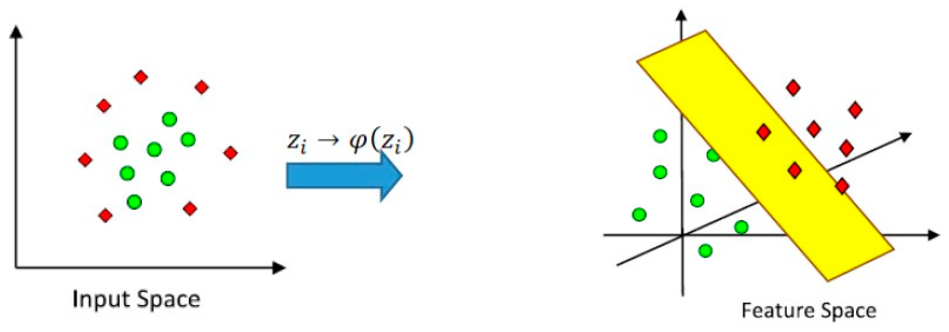
3.3. Support Vector Machine for the Non-Linear Case (Kernel Machine)

If input data are linearly separable, then it is easy to find the decision boundary to separate them into two or more classes based on the target feature. However, in most of the cases, the input data will not be linearly separable, and it would remain inappropriate to use linear decision boundary as a separator. To resolve this issue, input features are transformed onto a higher-dimensional space, given by Mercer (1909), and this concept is known as kernel method (Cristianini and Shawe-Taylor 2000). The input data will still be nonlinear, but the data can separate into two or more subspaces using an appropriate support vector classifier.
Figure 4 given below shows how the input data can be converted into a higher dimension by using kernel methods. The newly transformed coordinates show only the transformed data in a higher dimension. If z is the input data, then the transformed data in the new feature space are represented by ϕ ( z ) . The inner product of data in the new feature space is represented by a kernel function as in Figure 4.
ϕ ( z i , z j ) = K ( z i , z j )  

Kernel Trick

Equation (13) has been transformed into a new form for nonlinearly separable data using a kernel function and can be written as follows:
M a x       L d ( α ) = i = 1 N α i 1 2 i , j = 1 N y i y j α i α j K ( z i , z j ) s . t .                   { 0 α i C i = 1 N α i y i = 0
Here, “C” is the trade-off parameter included in Equation (15) to minimize the classification error and maximize the margin. We can find the optimal hyperplane using Equation (15). Using the new feature space, the weight vector “w” can be written as
w = i = 1 N y i α i ϕ ( z i )    
The bias term “b” is computed through the kernel function given as
b = y i i , j = 1 N S V y i α i K ( z i , z j )  
The hyperplane is defined as
h ( z ) = w T ϕ ( z ) + b
Using Equations (15)–(18), the equation of the hyperplane can be stated as
h ( z ) = i = 1 N y i α i K ( z , z i )   + b
In this paper, we used the SVM technique with the appropriate kernel as given in Table 1 to find the best predictive model and stress quantification.

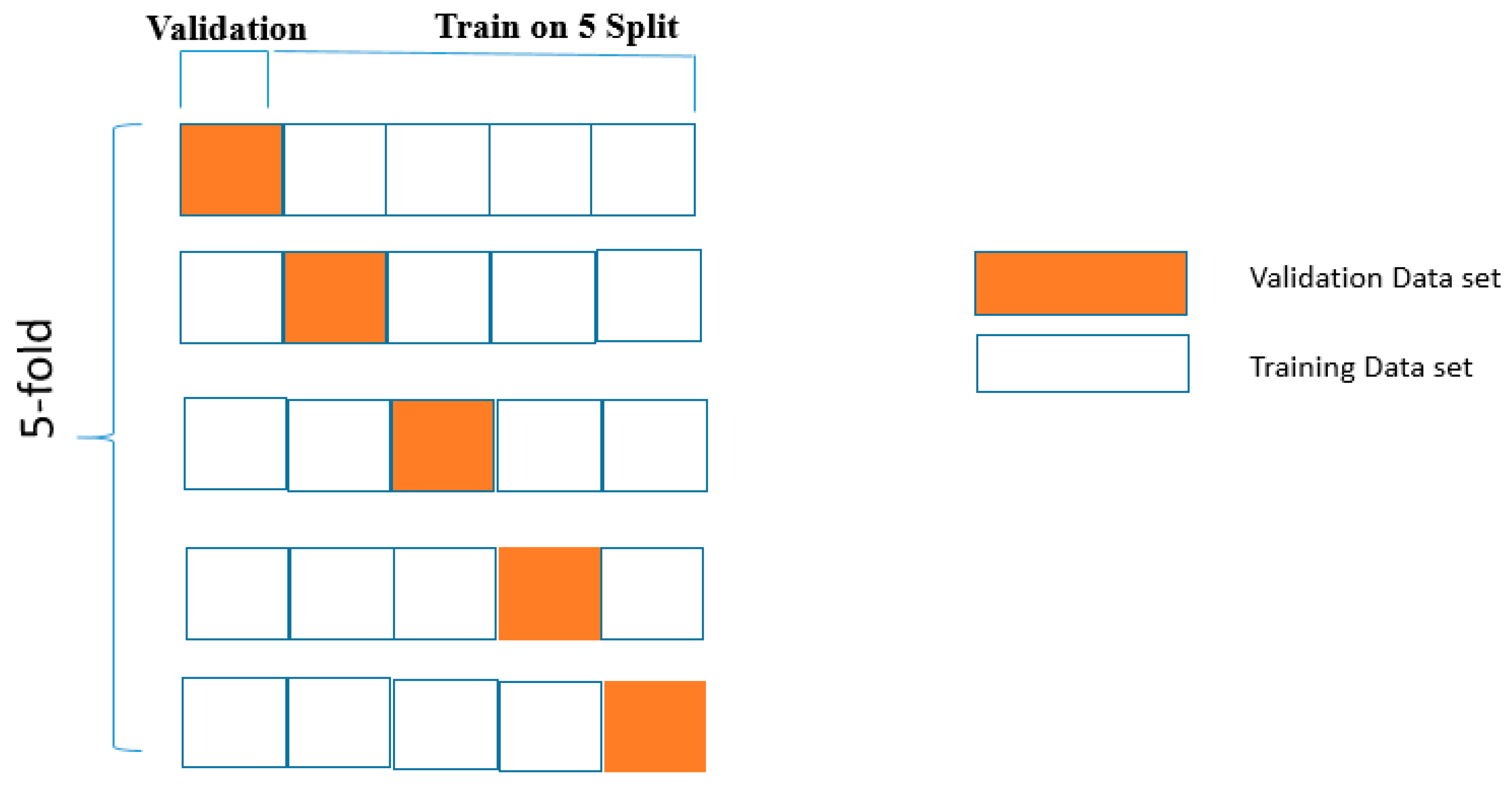
3.4. Overfitting and Cross-Validation

There is always a likelihood that the models may perform well on the training data but have poor performance for the unseen data. This case is known as overfitting. To resolve this issue, we used K-fold cross-validation in this study to overcome the problem of overfitting (Moore 2001).
K-fold cross-validation is a machine learning technique to check the stability and tune the parameters of the model. We divided the parent data into two parts in the proportions of 75% and 25% for training and testing data, respectively. We trained our model with training data and measured the accuracy of the testing data. In the case of K-Fold cross-validation, the input data were divided into “K” subsets, and we repeated this process “K” times. Out of k total subsets, one subset was used for the test set, and the remaining “K-1” subsets were used for training the methods. The algorithm error was calculated by taking the average of the error estimated during all “K” trials. By using this approach, we can eliminate the problem of overfitting. In this method, we used the 5-fold cross-validation technique, and the same is demonstrated in Figure 5.

4. Empirical Results and Discussion

4.1. Empirical Results

The first part of the feature selection is based on the relief algorithm that uses instance-based learning (Sun et al. 2009). The method calculates the weight for each feature as discussed in Section 3.1. In this method, the dependent variable is the financial position of banks classified as failed or survived. The important and useful features have relief scores greater than zero, and the redundant and non-significant features have relief scores either zero or less than zero. Sixteen out of 100 features have been selected based on relief scores as given in Table 2.
From Table 2 it is clear that, apart from recent information (t−1), some past information (t−2, t−3, and t−4) was also useful for bankruptcy prediction. The parent data were divided into two parts, training and testing, in the proportions of 75% and 25%, respectively. The training and testing data contained information of 44 and 14 banks, respectively. The model was formulated on the training data and validated on the testing dataset. With regards to the division of the data in training and testing sets, we maintained the same proportion of classes (failed or survived), as in the case of parent data. This was primarily to ensure that the weights between failed and survived classes were the same across all datasets.
In the second part of the feature selection method, we fed 16 features, given in Table 2, into SVM, and we refined the input features through the shrinking process. At each step, we compared the accuracy of the base feature set with all input features created by eliminating one input feature from the base input feature set. For instance, if the base feature set contained “p” features, we equated the base feature set with all probable sets of (p−1) input features. If the performance of the base feature set was not the best, then a (p–1) size feature set that gives the highest improvement on the base feature set swapped the base feature set in the next phase of iteration. This process remained until no progress was achieved by reducing the base feature set. Here, we tried only the two most common kernel functions: linear and radial basis function kernel (RBFK). We started iterations by taking all combinations from 16 features to obtain the best input in support vector machine with the linear kernel (SVMLK) and RBF kernel (SVMRK) at a time. SVMLK had the best accuracy with two explanatory features, Tier1CAR(t−1) and provision_for_loan_Interest_income(t−1), whereas SVMRK had the best accuracy with four explanatory features—subordebt_TA(t−1), Tier1CAR(t−1), provision_for_loan_Interest_income(t−2), and noninterest_expences_Int_income(t−3)—out of 16 features.
The best predictive results were achieved by SVMLK when the threshold value was 6.97. The SVMLK model gave 94.44% predictive accuracy, 75% sensitivity, and 100% specificity. The coefficients of input features for the linear decision boundary formed by SVMLK are mentioned below.
Input FeaturesCoefficient
provision_for_loan_Interest_income(t−1)6.056
Tier1CAR(t−1)4.37
Bias Term3.96
Cut-off value6.97
The failure and survival subspaces were divided based on the position of banks concerning the decision boundary. If the sum of the feature products and its coefficients with bias term was greater than 6.97, then the bank was classified as a survival bank, and a failed bank otherwise.
The SVMLK gave 100% accuracy for the surviving banks and 75% for failed banks, as shown in Table 3. The total accuracy of the SVMLK was 92.86%. The SVMRK gave 100% accuracy for the surviving banks and 0% for failed banks, as shown in Table 4. The total accuracy of the SVMRK was 71.43%. Our best model was obtained by using the SVMLK with an overall misclassification rate of 7.14%, while the best model with SVMRK had a 29.57% rate of misclassification. In the case of SVMLK, the best accuracy was obtained by using the features Tier1CAR(t−1) and provision_for_ loan_Interest_income(t−1), while in the case of SVMRK, the best accuracy was obtained by using the features subordebt_TA(t−1), Tier1CAR(t−1), provision_for_loan_Interest_income(t−2), and noninterest_expences_Int_income(t−3). In the case of SVMLK, both the features Tier1CAR(t−1) and provision_for_ loan_Interest_income(t−1) were recent information for the banks.

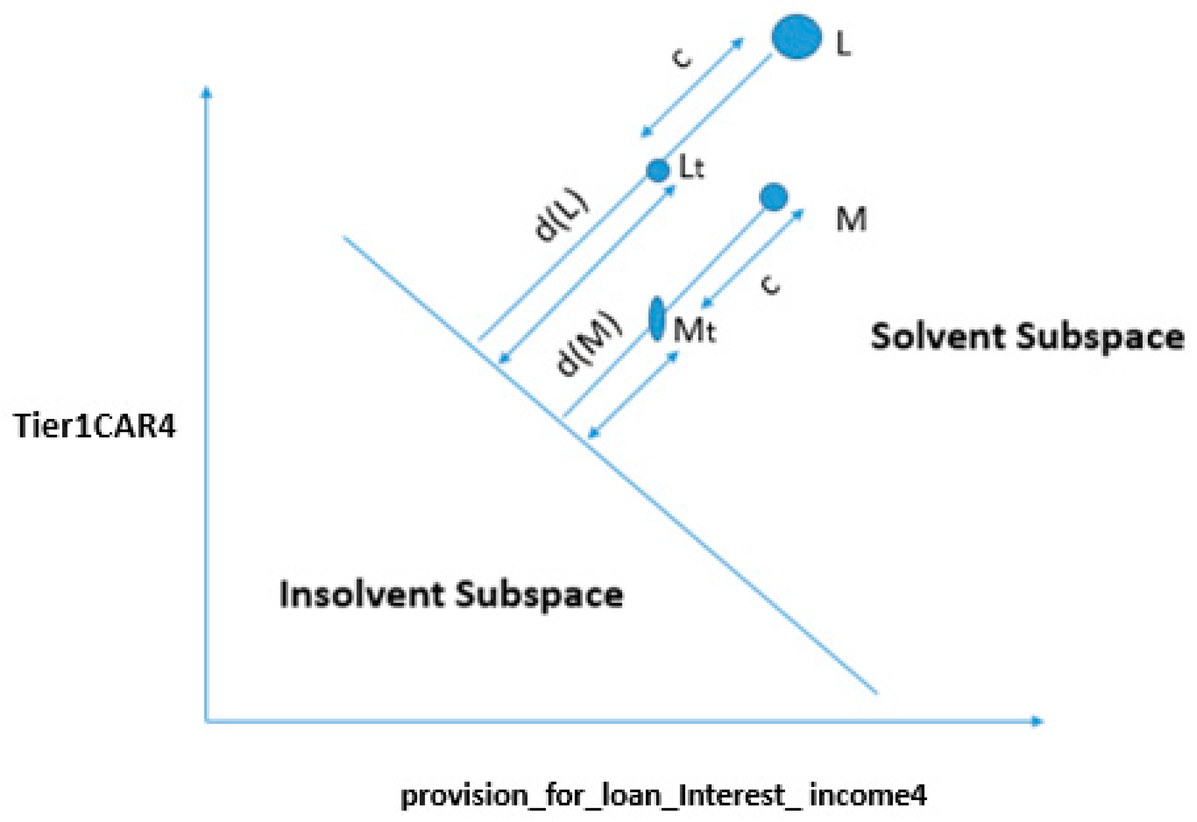
4.2. Stress Quantification of Banks

Decision Linear Boundary

It is clear from Section 4.1 that the SVMLK forecasting model gave the maximum accuracy. This model generated a hyperplane that classified the banks into two classes, solvent and insolvent, with two input features: (a) provision_for_loan_Interest_income(t−1) and (b) Tier1CAR(t−1). The mathematical equation of the linear hyperplane is
6.056 × provision_for_loan_Interest_income(t−1) + 4.37 × Tier1CAR(t−1) − 3.01 = 0, while the cut-off is scaled to zero.
Based on the above linear hyperplane given by the SVMLK model, we found the answer to some questions, as given below, by using geometrical interpretation.
(a)
By using the SVMLK predictive model, is it possible to find quantitative information about bank features to avoid a predicted bank failure?
(b)
How financially strong are the banks that are predicted as survival banks by using SVMLK predictive model?
Visualization of a decision boundary derived from SVM is easy when the kernel is linear and only two input features have been used.

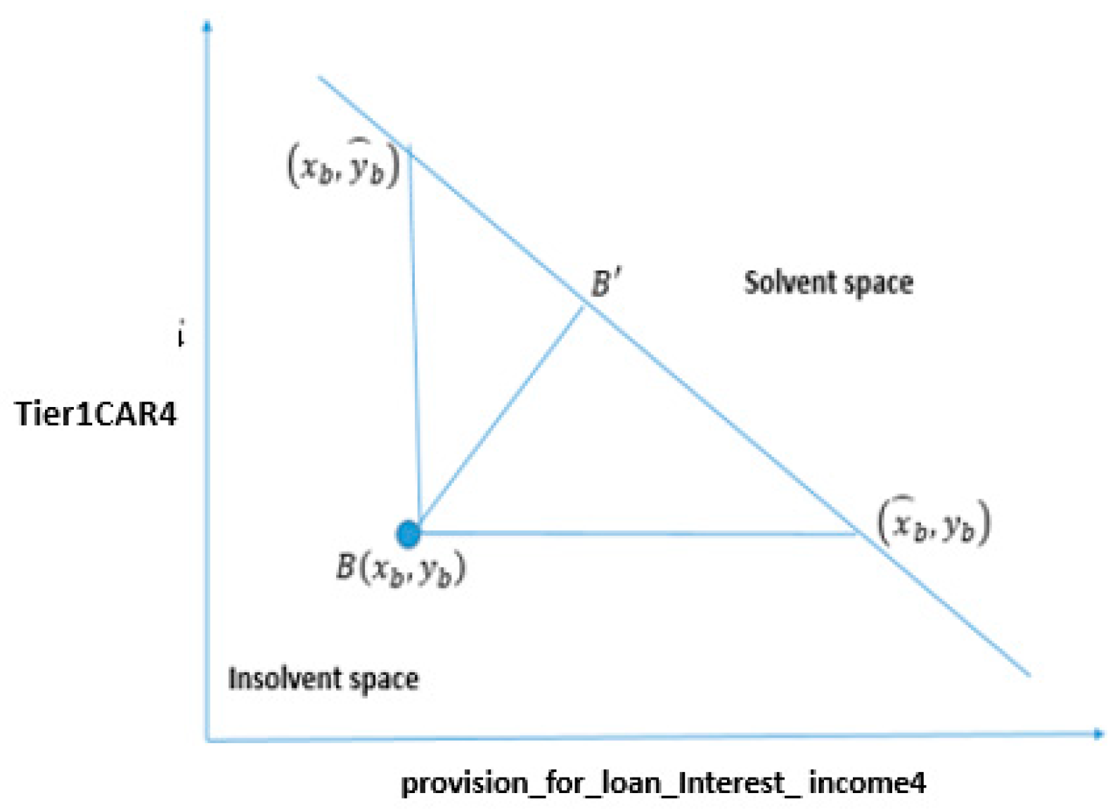
4.3. Mathematical Approach for Stress Quantification Using SVMLK

4.3.1. Change in Both Features

In this study, our focus was on the line (linear kernel) a x + b y + c = 0 , which divided the data into two classes: failure and survival. We take point B whose coordinates are ( x b , y b ) in the failed subspace, as shown in Figure 6, and if a x + b y + c = 0 is a decision boundary of the model, then the perpendicular distance of this point B ( x b , y b ) from the decision boundary is given by Equation (20).
d ( B , B ) = | a x b + b y b + c | a 2 + b 2  
The minimum distance that changes the position of point B ( x b , y b ) from failure to survival subspace is the perpendicular distance from point B to the line given in Equation (1).
The minimum change needed to move point B ( x b , y b ) from failure subspace to survival subspace is B ( x b a a x b + b y p + c a 2 + b 2 , y p b a x b + b y b + c a 2 + b 2 ) , and the difference in the coordinates of B and Bis given by B ( a a x p + b y p + c a 2 + b 2 , b a x p + b y p + c a 2 + b 2 ) .

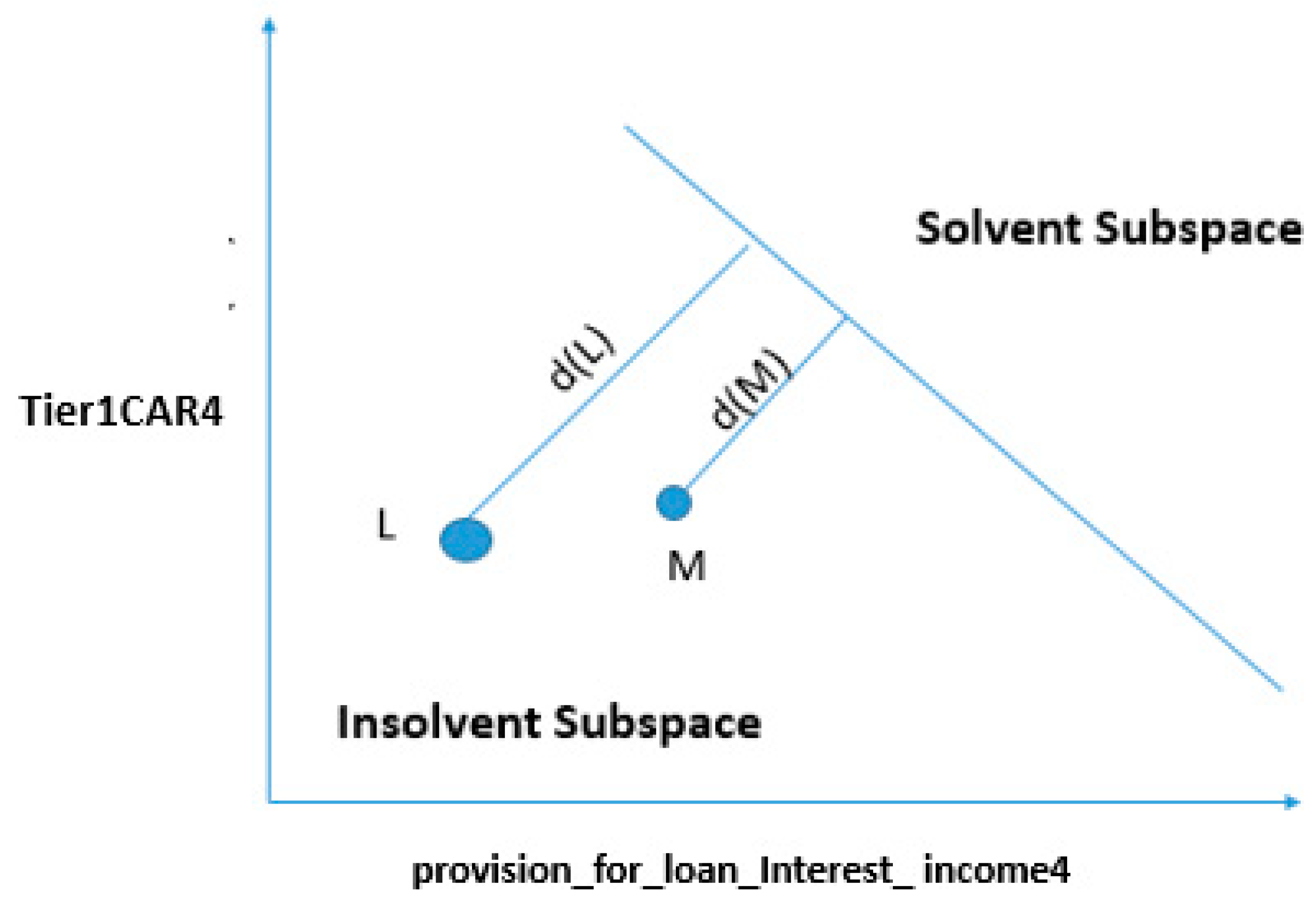
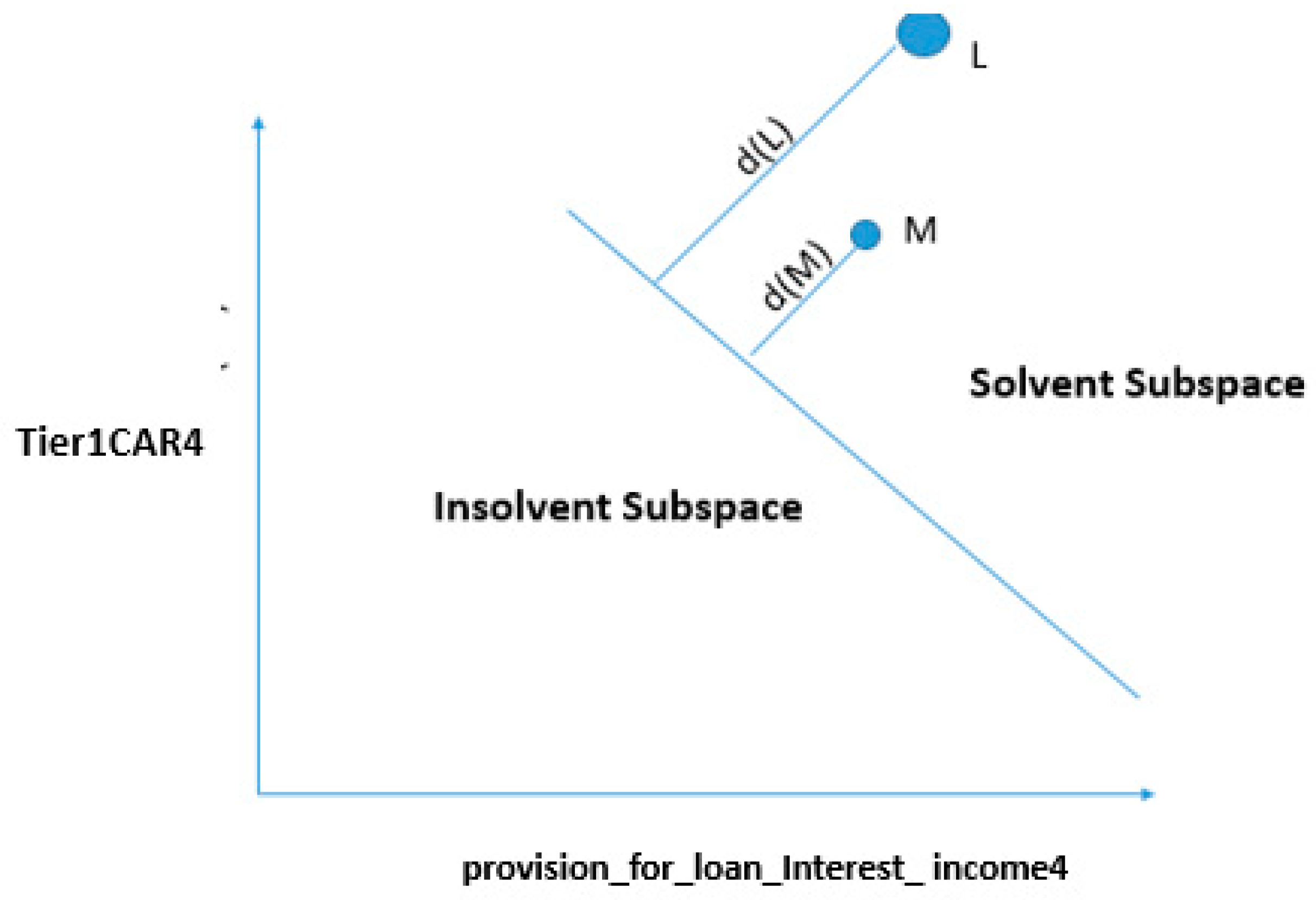
4.3.2. Change in One Feature

If we want to move point B from failure subspace to survival subspace by keeping one feature constant, say y b , then x b moves to the new point ( x b , y b ) , where a x b + b y b + c = 0 and x b = ( c b y b a ) = ( c + b y b a ) .
In another way, if we want to move point P from failure subspace to survival subspace by keeping x p , then y p moves to the new point ( x b , y ¯ b ) , where a x b + b y ¯ b + c = 0 and y ¯ b = ( c a x b b ) = ( c + a x b b ) .

4.4. Comparison of Bank Financial Health

From Section 4.3.1 and Section 4.3.2, we can determine the changes needed in the financial features of the bank under different situations that will change the forecasted position of the banks. Figure 7 represents the forecasted position of banks with two features: provision_for_loan_Interest_ income(t−1) and Tier1CAR(t−1).
If the two points L and M represent the banks forecasted as failed, and if d(L) > d(M), where d(L) and d(M) are the perpendicular distances from L and M to the decision boundary, as given in Figure 7, then this shows that bank L is financially weaker than bank M.
In another way, if the two points L and M represent the banks that are forecasted as surviving banks, and if d(L) > d(M), as given in Figure 8 where d(L) and d(M) are the perpendicular distances from L and M to the decision boundary, then this indicates that bank L is financially healthier in comparison to bank M.
Suppose that, due to some external financial environmental change, the perpendicular distance of point L and M from the linear decision boundary is reduced by amount “c”, then the new displaced points towards the boundary are Lt and Mt as shown in Figure 9.
If d (M) > c, both banks will be in survival subspace. If d (L) > c > d (M), the bank M lies in insolvent subspace, and bank L will still be healthy. If c > d (L), both banks L and M will lie in insolvent subspace. Based on the above analysis, we can conclude that the financial health of bank L is more sensitive in comparison to the financial health of bank M, and the distance of points L and M from the decision boundary shows the robustness or confidence about their financial health. This method can also be used by a monitoring committee to understand the different scenarios of the bank by making changes in financial features. The bank can determine the minimum changes required to avoid bankruptcy in the financial features and minimum changes required to move forecasted banks from failure subspace to survival subspace.
The value of the parameters “a”, “b”, and “c” for the decision boundary determined by SVMLK, as given in Equation (1), are 6.056, 4.37, and −3.01, respectively, where “a” is a coefficient of provision_for_loan_Interest_income(t−1), “b” is a coefficient of Tier1CAR(t−1), and “c” is a bias term. The decision boundary equation is given by
6.056 × provision_for_loan_Interest_income(t−1) + 4.37 × Tier1CAR(t−1) − 3.01 = 0.
The perpendicular distance from point B (provision_for_loan_Interest_income(t−1), Tier1CAR(t−1)) to the decision boundary is given by
d ( B , B ) = | 6.056 × p r o v i s i o n _ f o r _ l o a n _ I n t e r e s t _ i n c o m e ( t 1 ) + 4.37 × T i e r 1 C A R ( t 1 ) 3.01 | 6.056 ^ 2 + 4.37 ^ 2  
Using Equation (21), we calculated the distance of banks which were forecasted as solvent and insolvent from the decision boundary. The minimum and maximum distances of banks forecasted as solvent from the linear decision boundary were 8.53 and 29.52, while the minimum and maximum distances of banks forecasted as insolvent from the linear decision boundary were 4.02 and 10.86. Based on these distances, we used sensitivity analysis to quantify the amount of stress based on two important bank features: provision_for_loan_Interest_income(t−1) and Tier1CAR(t−1).
Here, we will take an example to understand the applicability of stress quantification. We will not disclose the name of the bank in order to maintain secrecy. For example, bank “A”, which has been predicted by the model as the failed bank, is selected for stress quantification. The values of the features provision_for_loan_Interest_income(t−1) and Tier1CAR(t−1) are (0.00123, 0.1120) for bank “A”. The position of bank “A” with respect to the decision boundary of SVMLK lies in the insolvency region.

4.4.1. Changing the Status of Bank “A” from Insolvent to Solvent by Changing Both Variables

Table 5 lists the original values of the two features provision_for_loan_Interest_income(t−1) and Tier1CAR(t−1) of bank “A” as well as its critical values to move from solvent subspace to insolvent subspace. These critical values quantify the amount of provision_for_loan_Interest_income(t−1) and Tier1CAR(t−1) needed to cross the decision boundary of insolvent to the solvent subspace.
The minimum changes required in provision_for_loan_Interest_income(t−1) and Tier1CAR(t−1) to move bank “A” from insolvent subspace to solvent subspace is (2.0, 1.60).

4.4.2. Marginal Cases: Changing the Status of Bank “A” from Insolvent to Solvent by Changing a Single Variable

Case 1.
In this case, we kept the second feature Tier1CAR(t−1) constant while changing the value of the first feature provision_for_loan_Interest_income(t−1).
FeaturesOriginal ValuesCritical Values
provision_for_loan_Interest_income(t−1)0.001230.49
Tier1CAR(t−1)0.11230.1123
Based on the distance measure of bank “A” from the decision boundary, we can calculate the minimum changes required to move bank “A” from insolvent to solvent subspace. The critical values of the two features provision_for_loan_Interest_income(t−1) and Tier1CAR(t−1) were 0.00123 and 0.1120. Based on the critical values, we can conclude that bank “A” should maintain the provision_for_loan_Interest_income(t−1) more than 0.49 by keeping Tier1CAR(t−1) constant to move the status of Bank “A” from insolvent to solvent subspace.
Case 2.
In this case, we kept the first feature provision_for_loan_Interest_income(t−1) constant while changing the value of the second feature Tier1CAR(t−1).
FeaturesOriginal ValuesCritical Values
provision_for_loan_Interest_income(t−1)0.001230.00123
Tier1CAR(t−1)0.11230.54
If we change Tier1CAR(t−1) by keeping provision_for_loan_Interest_income(t−1) constant, then the bank should keep the value of Tier1CAR(t−1) more than 0.54 to move from insolvent subspace to solvent subspace. If we arrange the rank of the banks forecasted as failed based on the distance from decision boundary, then the bank with a rank of one (higher distance from decision boundary) will feel more financial stress in comparison to rank two and so on. Similarly, if we arrange the rank of the banks forecasted as survived based on the distance from decision boundary, then the bank having a higher rank (higher distance from decision boundary) will feel more financial security in comparison to lower-ranked banks.
By using this SVMLK and rank-based approach, each bank is classified as “solvent” or “insolvent”, and banks are ranked based on the distance from the decision boundary. The result of this study may prove useful for managers and the government for micro-level supervision. This method of stress quantification is useful to create an early warning for banks that are likely to fail soon.

5. Conclusions

Early warning of potential bank failure is important for various stakeholders like management personnel, lenders, and shareholders. In this study, we used the support vector machine to predict the financial status of banks. We used a two-step feature selection relief algorithm and support vector machine to arrive at the best predictive model. The accuracies of SVMLK and SVMRK on the sample data were found to be 92.86% and 71.43%, respectively. Based on the predictive accuracy of these two models, we concluded that SVMLK is a better predictive model than SVMRK and uses two features, provision_for_loan_Interest_income(t−1) and Tier1CAR(t−1). Further, by using SVMLK, we used the proposed stress quantification technique to compare the financial health of banks. We also used a geometrical interpretation of the decision boundary of SVMLK to measure the minimum changes required for banks to move from failure subspace to survival subspace. This, in turn, will help bank management to take appropriate steps to avoid possible bankruptcy in the future.

6. Limitations of the Study

As stated earlier in this study, the number of failed banks in India is found to be relatively low. Hence, data available for failed banks may seem to be relatively limited compared to that of surviving banks. This data imbalance is one of the major limitations of the SVM model used in this study. Another important limitation of the study is that, if the model is replicated with other firms, one may get other forms of SVM than SVMLK; thus, interpretation of the results would be difficult. Another limitation we foresee is that it is possible to get a different combination of features while working on the datasets of firms in other countries. This could be due to various country-specific reasons like government policies, economic indicators, and so forth.

Author Contributions

The authors have equal contributions. All authors have read and agreed to the published version of the manuscript.

Funding

This research received no external funding.

Conflicts of Interest

The authors declare no conflict of interest.

Appendix A

Table A1. List of 25 features calculated for banks.
NameTypeDefinition
Financial Status
(Failed or Survival)
Categorical Binary indicator equal to 1 for failed banks and 0 for surviving banks
Total_Assets (TA)QuantitativeTotal earning assets
Cash_Balance_TAQuantitativeCash and due from depository institutions/TA
Net_Loan_TAQuantitativeNet loans /TA
Deposit_TAQuantitativeTotal Deposits/TA
Subordinated_debt_TAQuantitativeSubordinated Debt/TA
Average_Assets_TAQuantitativeAverage Assets till 2017/Total Assets
Tier1CARQuantitativeTier1 risk-based capital/Total Assets
Tier2CARQuantitativeTier 2 risk-based capital/Total Assets
IntincExp_IncomeQuantitativeTotal interest expense/total interest income
Provision_for_loan_Interest_incomeQuantitativeProvision for loan and lease losses/total interest income
Nonintinc_intIncomeQuantitativeTotal noninterest income/total interest income
Return_on_capital_employedQuantitativeSalaries and employee benefits/total interest income
Operating_income_T_Interest_incomeQuantitativenet operating income/total interest income
Cash_dividend_T_Interest_IncomeQuantitativeCash dividends/total interest income
Operating_income_T_Interest_incomeQuantitativeNet operating income/total interest income
Net_Interest_marginQuantitativeNet interest margin earned by bank
Return_on_assetsQuantitativeReturn on total assets of firm
Equity_cap_TAQuantitativeEquity capital to assets
Return_on_AssetsQuantitativeReturn on total assets of banks
Noninteerst_IncomeQuantitativeNoninterest Income earned by banks
Treasury_income_T_Interest_incomeQuantitativeNet income attributable to bank/total interest income
Net_loans_DepositsQuantitativeNet loans and leases to deposits
Net_Interest_marginQuantitativeNet interest income expressed as a percentage of earning assets.
Salaries_employees_benefits_Int_incomeQuantitativeSalaries and employee benefits/total interest income
TA_employeeQuantitativeTotal assets per employee of bank

Appendix B

Table A2. List of 100 features and weights calculated by the relief algorithm.
Variables NameRelief Score
Tier1CAR(t−1)0.18
Subordebt_TA(t−1)0.12
Tier2CAR(t−2)0.1
Provision_for_loan_Interest_income(t−4)0.1
Subordebt_TA(t−3)0.09
Provision_for_loan_Interest_income(t−1)0.08
Provision_for_loan_Interest_income(t−2)0.08
Provision_for_loan_Interest_income(t−3)0.07
TA_emplyee(t−3)0.07
TA_emplyee(t−2)0.06
Tier2CAR(t−1)0.06
TA_emplyee(t−4)0.05
TA_emplyee(t−1)0.05
Noninterest_expences_Int_income(t−3)0.04
Subordebt_TA(t−4)0.02
Salaries_and_employees_benefits_Int_income(t−3)0.01
Tier2CAR(t−3)0.00
Return_on_capital_employed_(t−2)0.00
Operating_income_T_Interest_income(t−4)0.00
Cash_TA(t−3)0.00
Noninterest_expences_Int_income(t−4)0.00
Deposits_TA(t−2)0.00
Return_on_advances_adjusted_to_cost_of_funds(t−1)0.00
Operating_income_T_Interest_income(t−3)0.00
Return_on_capital_employed(t−3)0.00
Salaries_and_employees_benefits_Int_income(t−4)0.00
Net_loans_TA(t−3)0.00
Deposits_TA(t−1)0.00
Treasury_income_T_Interest_income(t−4)0.00
Return_on_assets(t−3)0.00
Net_loans_TA(t−2)0.00
Net_loans_TA(t−1)0.00
Return_on_assets(t−1)0.00
Return_on_capital_employed(t−4)0.00
IntincExp_Income(t−2)0.00
Cash_TA(t−2)0.00
IntincExp_Income(t−4)0.00
Noninterest_expences_Int_income(t−1)0.00
Return_on_advances_adjusted_to_cost_of_funds(t−2)0.00
Nonintinc_intIncome(t−4)0.00
Nonintinc_intIncome(t−1)0.00
Deposits_TA(t−3)0.00
Equity_cap_TA(t−1)0.00
IntincExp_Income(t−3)0.00
Operating_income_T_Interest_income(t−1)0.00
Avg_Asset_TA(t−2)0.00
Total_Assets(t−3)0.00
Noninteerst_Income(t−3)0.00
Provision_for_loan(t−2)0.00
Total_Assets(t−4)0.00
Salaries_and_employees_benefits_Int_income(t−1)0.00
Noninteerst_Income(t−2)0.00
Total_Assets(t−1)0.00
Return_on_capital_employed(t−1)0.00
Noninteerst_Income(t−4)0.00
Subordebt_TA(t−2)0.00
Total_Assets(t−2)0.00
Noninterest_expences_Int_income(t−2)0.00
Equity_cap_TA(t−2)0.00
Noninteerst_Income(t−1)0.00
Salaries_and_employees_benefits_Int_income(t−2)0.00
Nonintinc_intIncome(t−3)0.00
Treasury_income_T_Interest_income(t−3)0.00
Return_on_assets(t−4)0.00
Treasury_income_T_Interest_income(t−1)0.00
Tier1CAR(t−3)0.00
Avg_Asset_TA(t−3)0.00
Tier1CAR(t−4)0.00
Equity_cap_TA(t−3)0.00
IntincExp_Income(t−1)0.00
Return_on_assets(t−2)0.00
Treasury_income_T_Interest_income(t−2)0.00
Net_Interest_margin(t−4)0.00
Tier1CAR(t−2)0.00
Cash_TA(t−1)0.00
Provision_for_loan(t−4)0.00
Net_Interest_margin(t−2)0.00
Net_Interest_margin(t−1)0.00
Cash_TA(t−4)0.00
Deposits_TA(t−4)0.00
Equity_cap_TA(t−4)0.00
Net_loans_TA(t−4)0.00
Return_on_advances_adjusted_to_cost_of_funds(t−4)0.00
Return_on_advances_adjusted_to_cost_of_funds(t−3)0.00
Provision_for_loan(t−3)0.00
Avg_Asset_TA(t−4)0.00
Operating_income_T_Interest_income(t−2)0.00
Net_loans_Deposits(t−3)0.00
Nonintinc_intIncome(t−2)0.00
Net_Interest_margin(t−4)0.00
Net_loans_Deposits(t−4)0.00
Avg_Asset_TA(t−1)0.00
Tier2CAR(t−4)−0.01
Net_loans_Deposits(t−2)−0.01
Cash_dividend_T_Interest_Income(t−2)−0.01
Cash_dividend_T_Interest_Income(t−1)−0.01
Cash_dividend_T_Interest_Income(t−4)−0.01
Net_loans_Deposits(t−1)−0.01
Cash_dividend_T_Interest_Income(t−3)−0.02

References

  1. Aha, David W., Dennis Kibler, and Marc K. Albert. 1991. Instance-based learning algorithms. Machine Learning 6: 37–66. [Google Scholar] [CrossRef] [Green Version]
  2. Altman, Edward I. 1968. Financial ratios, discriminant analysis and the prediction of corporate bankruptcy. The Journal of Finance 23: 589–609. [Google Scholar] [CrossRef]
  3. Altman, Edward I., Robert G. Haldeman, and Paul Narayanan. 1977. ZETATM analysis A new model to identify bankruptcy risk of corporations. Journal of Banking & Finance 1: 29–54. [Google Scholar]
  4. Altman, Edward I., Marco Giancarlo, and Giancarlo Varetto. 1994. Corporate distress diagnosis: Comparisons using linear discriminant analysis and neural networks (the Italian experience). Journal of Banking & Finance 18: 505–29. [Google Scholar]
  5. Antunes, Francisco, Bernardete Ribeiro, and Bernardete Pereira. 2017. Probabilistic modeling and visualization for bankruptcy prediction. Applied Soft Computing 60: 831–43. [Google Scholar] [CrossRef] [Green Version]
  6. Chaudhuri, Arindam, and Kajal De. 2011. Fuzzy support vector machine for bankruptcy prediction. Applied Soft Computing 11: 2472–86. [Google Scholar] [CrossRef]
  7. Chen, Ning, Bernardete Ribeiro, Armando Vieira, and An Chen. 2013. Clustering and visualization of bankruptcy trajectory using self-organizing map. Expert Systems with Applications 40: 385–93. [Google Scholar] [CrossRef]
  8. Cleary, Sean, and Greg Hebb. 2016. An efficient and functional model for predicting bank distress: In and out of sample evidence. Journal of Banking & Finance 64: 101–11. [Google Scholar]
  9. Cole, Rebel A., and Jeffery Gunther. 1995. A CAMEL Rating’s Shelf Life. Available at SSRN 1293504. Amsterdam: Elsevier. [Google Scholar]
  10. Cole, Rebel A., and Jeffery W. Gunther. 1998. Predicting bank failures: A comparison of on-and off-site monitoring systems. Journal of Financial Services Research 13: 103–17. [Google Scholar] [CrossRef]
  11. Cortes, Corinna, and Vladimir Vapnik. 1995. Support-vector networks. Machine Learning 20: 273–97. [Google Scholar] [CrossRef]
  12. Cristianini, Nello, and John Shawe-Taylor. 2000. An Introduction to Support Vector Machines (and Other Kernel-Based Learning Methods). Cambridge: Cambridge University Press, 190p. [Google Scholar]
  13. Dash, Mihir, and Annyesha Das. 2009. A CAMELS Analysis of the Indian Banking Industry. Available at SSRN 1666900. Amsterdam: Elsevier. [Google Scholar]
  14. Du Jardin, Philippe. 2012. Predicting bankruptcy using neural networks and other classification methods: The influence of variable selection techniques on model accuracy. Neurocomputing 73: 2047–60. [Google Scholar] [CrossRef] [Green Version]
  15. Fletcher, Desmond, and Ernie Goss. 1993. Forecasting with neural networks: an application using bankruptcy data. Information & Management 24: 159–67. [Google Scholar]
  16. Kim, Myoung-Jong, Dae-Ki Kang, and Hong Bae Kim. 2015. Geometric mean based boosting algorithm with over-sampling to resolve data imbalance problem for bankruptcy prediction. Expert Systems with Applications 42: 1074–82. [Google Scholar] [CrossRef]
  17. Kira, Kenji, and Larry A. Rendell. 1992. A practical approach to feature selection. In Machine Learning Proceedings 1992. Amsterdam: Elsevier, pp. 249–56. [Google Scholar]
  18. Kirkos, Efstathios. 2015. Assessing methodologies for intelligent bankruptcy prediction. Artificial Intelligence Review 43: 83–123. [Google Scholar] [CrossRef]
  19. Korol, Tomasz. 2013. Early warning models against bankruptcy risk for Central European and Latin American enterprises. Economic Modelling 31: 22–30. [Google Scholar] [CrossRef]
  20. Leshno, Moshe, and Yishay Spector. 1996. Neural network prediction analysis: The bankruptcy case. Neurocomputing 10: 125–47. [Google Scholar] [CrossRef]
  21. Lin, Wei-Yang, Ya-Han Hu, and Chih-Fong Tsai. 2011. Machine learning in financial crisis prediction: a survey. IEEE Transactions on Systems, Man, and Cybernetics, Part C (Applications and Reviews) 42: 421–36. [Google Scholar]
  22. Mangasarian, Olvi. L. 1969. Nonlinear Programming. New York: McGraw-Hill Book Co. [Google Scholar]
  23. Martin, Daniel. 1977. Early warning of bank failure: A logit regression approach. Journal of Banking & Finance 1: 249–76. [Google Scholar]
  24. Meyer, Paul A., and Howard W. Pifer. 1970. Prediction of bank failures. The Journal of Finance 25: 853–68. [Google Scholar] [CrossRef]
  25. Mercer, James. 1909. Functions of positive and negative type and their connection with the theory of integral equations. Philosophical Transactions of the Royal Society A 209: 415–46. [Google Scholar]
  26. Moore, Andrew W. 2001. Cross-Validation for Detecting and Preventing Overfitting. Pittsburgh: School of Computer Science Carneigie Mellon University. [Google Scholar]
  27. Murphy, Kevin P. 2012. Machine Learning: A Probabilistic Perspective. Cambridge: MIT Press. [Google Scholar]
  28. Nanni, Loris, and Alessandra Lumini. 2009. An experimental comparison of ensemble of classifiers for bankruptcy prediction and credit scoring. Expert Systems with Applications 36: 3028–33. [Google Scholar] [CrossRef]
  29. Ohlson, James A. 1980. Financial ratios and the probabilistic prediction of bankruptcy. Journal of Accounting Research 18: 109–31. [Google Scholar] [CrossRef] [Green Version]
  30. Papadimitriou, Theophilos, Periklis Gogas, Vasilios Plakandaras, and John C. Mourmouris. 2013. Forecasting the insolvency of US banks using support vector machines (SVM) based on local learning feature selection. International Journal of Computational Economics and Econometrics 3: 1. [Google Scholar] [CrossRef]
  31. Pappas, Vasileios, Steven Ongena, Marwan Izzeldin, and Ana-Maria Fuertes. 2017. A survival analysis of Islamic and conventional banks. Journal of Financial Services Research 51: 221–56. [Google Scholar] [CrossRef] [Green Version]
  32. Piramuthu, Selwyn, Harish Ragavan, and Michael J. Shaw. 1998. Using feature construction to improve the performance of neural networks. Management Science 44: 416–30. [Google Scholar] [CrossRef]
  33. Pradhan, Roli. 2014. Z score estimation for Indian banking sector. International Journal of Trade, Economics, and Finance 5: 516. [Google Scholar] [CrossRef] [Green Version]
  34. Chelimala, Pramodh, and Vadlamani Ravi. 2007. Modified great deluge algorithm based auto-associative neural network for bankruptcy prediction in banks. International Journal of Computational Intelligence Research 3: 363–71. [Google Scholar]
  35. Sharda, Ramesh, and Rick L. Wilson. 1993. Performance comparison issues in neural network experiments for classification problems. In [1993] Proceedings of the Twenty-Sixth Hawaii International Conference on System Sciences. Piscataway: IEEE, vol. 4, pp. 649–57. [Google Scholar]
  36. Shrivastav, Santosh Kumar. 2019. Measuring the Determinants for the Survival of Indian Banks Using Machine Learning Approach. FIIB Business Review 8: 32–38. [Google Scholar] [CrossRef]
  37. Shrivastava, Santosh, P. Mary Jeyanthi, and Sarabjit Singh. 2020. Failure prediction of Indian Banks using SMOTE, Lasso regression, bagging and boosting. Cogent Economics & Finance 8: 1729569. [Google Scholar]
  38. Shumway, Tyler. 2001. Forecasting bankruptcy more accurately: A simple hazard model. The Journal of Business 74: 101–24. [Google Scholar] [CrossRef] [Green Version]
  39. Sun, Yijun, Sinisa Todorovic, and Steve Goodison. 2009. Local-learning-based feature selection for high-dimensional data analysis. IEEE Transactions on Pattern Analysis and Machine Intelligence 32: 1610–26. [Google Scholar]
  40. Swicegood, Philip, and Jeffrey A. Clark. 2001. Off-site monitoring systems for predicting bank underperformance: a comparison of neural networks, discriminant analysis, and professional human judgment. Intelligent Systems in Accounting, Finance & Management 10: 169–86. [Google Scholar]
  41. Tam, Kar Yan. 1991. Neural network models and the prediction of bank bankruptcy. Omega 19: 429–45. [Google Scholar] [CrossRef]
  42. Tian, Yingjie, Yong Shi, and Xiaohui Liu. 2012. Recent advances on support vector machines re-search. Technological and Economic Development of Economy 18: 5–33. [Google Scholar] [CrossRef] [Green Version]
  43. Tsukuda, Junsei, and Shin-ichi Baba. 1994. Predicting Japanese corporate bankruptcy in terms of financial data using neural network. Computers & Industrial Engineering 27: 445–48. [Google Scholar]
  44. Vapnik, Vladimir. 1998. The support vector method of function estimation. In Nonlinear Modeling. Boston: Springer, pp. 55–85. [Google Scholar]
  45. Wang, Gang, Jinxing Hao, Jian Ma, and Hongbing Jiang. 2011. A comparative assessment of ensemble learning for credit scoring. Expert Systems with Applications 38: 223–30. [Google Scholar] [CrossRef]
  46. Wang, Gang, Jian Ma, and Shanlin Yang. 2014. An improved boosting based on feature selection for corporate bankruptcy prediction. Expert Systems with Applications 41: 2353–61. [Google Scholar] [CrossRef]
  47. Whalen, Gary. 1991. A proportional hazards model of bank failure: an examination of its usefulness as an early warning tool. Economic Review 27: 21–31. [Google Scholar]
  48. Yeh, Quey-Jen. 1996. The application of data envelopment analysis in conjunction with financial ratios for bank performance evaluation. Journal of the Operational Research Society 47: 980–88. [Google Scholar] [CrossRef]
  49. Zmijewski, Mark E. 1984. Methodological issues related to the estimation of financial distress prediction models. Journal of Accounting Research 22: 59–82. [Google Scholar] [CrossRef]
Figure 1. The case of hard margin where data are easily separable.
Risks 08 00052 g001
Figure 2. Linear decision boundary with two explanatory variables x1 and x2.
Risks 08 00052 g002
Figure 3. Represents the case of soft margin where data are not easily separable.
Risks 08 00052 g003
Figure 4. Transforming input features from a lower dimension to a higher dimension.
Risks 08 00052 g004
Figure 5. 5-fold cross-validation.
Risks 08 00052 g005
Figure 6. Representation of stress quantification. The x-axis denotes the provision_for_loan_Interest_income(t−1) and the y-axis represents Tier1CAR(t−1).
Risks 08 00052 g006
Figure 7. Quantifying and comparing the financial health of failed banks.
Risks 08 00052 g007
Figure 8. Quantifying and comparing the financial health of surviving banks.
Risks 08 00052 g008
Figure 9. Quantifying and comparing the financial health of surviving banks after the environmental change.
Risks 08 00052 g009
Table 1. Kernel functions.
Mathematical Kernel EquationName of Kernel
K ( z i , z j ) = ( z i T z j + p ) Linear
K ( z i , z j ) = exp ( α [ z i z j 2 ] ) RBF (Radial Basis Function)
Here p and α are the hyperplane parameters and need to be optimized.
Table 2. List of features with positive weights assigned by the relief algorithm.
Subordebt_TA (t−2)0.18
Subordebt_TA (t−1)0.12
Tier1CAR(t−2)0.1
Provision_for_loan_Interest_income (t−4)0.1
Subordebt_TA(t−3)0.09
Provision_for_loan_Interest_income(t−1)0.08
Provision_for_loan_Interest_income(t−2)0.08
Provision_for_loan_Interest_income(t−3)0.07
TA_employee(t−3)0.07
TA_employee(t−2)0.06
Tier1CAR(t−1)0.06
TA_employee(t−4)0.05
TA_employee(t−1)0.05
Noninterest_expences_Int_income(t−3)0.04
Subordebt_TA(t−4)0.02
Salaries_and_employees_benefits_Int_income(t−3)0.01
Table 3. Overall accuracy of SVMLK on the testing dataset.
Total AccuracySolvent Predictive AccuracyInsolvent Predictive Accuracy
92.86%100%75%
Table 4. Overall accuracy of SVMRK on the testing dataset.
Total AccuracySolvent Predictive AccuracyInsolvent Predictive Accuracy
71.43%100%0%
Table 5. Features, original values, and critical values.
FeaturesOriginal Values Critical Values
provision_for_loan_Interest_income(t−1)0.001232.0
Tier1CAR(t−1)0.11231.6

