Abstract
This paper examines the impact of the parameters of the distribution of the time at which a bank’s client defaults on their obligated payments, on the Lundberg adjustment coefficient, the upper and lower bounds of the ruin probability. We study the corresponding ruin probability on the assumption of (i) a phase-type distribution for the time at which default occurs and (ii) an embedding of the stochastic cash flow or the reserves of the bank to the Sparre Andersen model. The exact analytical expression for the ruin probability is not tractable under these assumptions, so Cramér Lundberg bounds types are obtained for the ruin probabilities with concomitant explicit equations for the calculation of the adjustment coefficient. To add some numerical flavour to our results, we provide some numerical illustrations.
1. Introduction
Credit risk affects the banking sector and may lead to global economic stagnation (Nkusu 2011). This was demonstrated convincingly by the 2007 subprime mortgage crisis whereby mortgages to clients who were likely to default were repackaged by lenders into mortgage-backed securities and sold to investors in exchange for regular income payments (Longstaff 2010). When the housing bubble burst, the inevitable default occurred and a domino effect was set in motion (see Mohan 2009). For an empirical investigation of the strong evidence of this domino effect of the collapse of the financial markets to the global economy see Longstaff (2010). This crisis led banks to improve their credit risk control by moving from a rules-based systems to a principles-based system. The latter tends to provide a better reflection of a financial institution’s true risk situation by employing various risk measures to reduce the number of potential client defaults.
In the financial literature, there are many models and approaches that have been adopted to measure risks. Prominent among them are ruin theory models. Originally developed for the insurance industry, the ruin probability is used to study the stochastic processes that represent the time evolution of the surplus and serve as the main risk measure to quantify the solvency of the company. After the global crisis (2007–2008), European Union regulatory board established new principles called the Basel II (respectively solvency II for insurance sector) accords to strengthen the previous solvency system (Basel I respectively solvency I) in terms of risk management principles. Under solvency II, insurance companies are required to fulfill certain capital adequacy rations in order for them to sell any contracts. Maintenance of the solvency capital requirement (SCR) coverage ratio enables the financial institution to stay above a certain threshold with a large enough probability. Although internal and standard models exist to determine this ratio, they are complex and time consuming. An alternative way to handle this problem is to use the ruin probability to study the capital requirement in numerous adverse scenarios without varying the probability of these scenarios as the ruin formula is explicitly known under some specific assumptions. Thus the ruin probability is considered as an important type of risk measure. Quaigrain (2013) showed that one can apply this risk measure more broadly in finance. For example, risk measures can be used to address the adequacy of the assets, as shown in Cody (1988) where the ruin probability has been used to analyse the cash flow scenarios of reasonable and plausible deviations from expectation with bounding worst scenarios. Further, it can also be used to analyze the liquidity requirement for financial futures investments. Kolb et al. (1985), showed that the ruin probability increases with the length of the hedging horizon and varies with the maturity of the contract being trade. Finally, by embedding the stochastic cash flow of the customer to the Sparre Andersen model, Cramér Lundberg bounds for the ruin probability can be derived.
The mathematical fundamentals of ruin theory were originally addressed by Lundberg (1903, 1909). In his papers he established the upper bound of ruin probability through the classical compound Poisson risk model. Later, Cramér (1926, 1930) extended Lundberg’s work when he derived the probability of the surplus being negative.
The ruin probability of the insurance cash flow process and its related functionals has been the subject of several studies, especially within the renewal context. The reader is referred to Andersen (1957); Gerber (1979); Grandell (1991); Bühlmann (2007) and references therein. In particular Andersen (1957) established renewal process by extending the compound Poisson model by allowing the inter-arrival times to have any arbitrary distribution. Dickson (1994) extended Lundberg and Cramér’s work and derived an upper bound for the ruin probability in the classical compound Poisson model where the moment generating function of the claim amounts exists. Although an explicit formula for the ruin probability is hard to obtain in many scenarios it exists under some specific assumption such as an exponential distribution for the claim amount in the classical renewal process or an Erlang inter-arrival with Pareto claim distribution (see Burnecki et al. 2005; Ramsay 2003; Wei and Yang 2004). In the case where explicit formula does not exist, the ruin probability can be approximated or bounded using Cramér Lundberg types bounds.
Since the exact claim distribution is crucial for the accuracy of the model while using ruin probability as risk measure, it must be chosen with care so that it can fit the real data. In the literature many distributions are suggested to model the claim distribution. Examples are exponential, gamma, Erlang, Weibull, Pareto, to name a few. It is well known that any positive distribution can be approximated by a phase-type distribution. This type of distribution can be used to model the claim amount. An introduction to this type of distribution can be found in Buchholz et al. (2014) and references therein. The originator of the phase-type distribution in stochastic modelling is Neut who introduced this concept in queue modelling (Neuts 1981). Further to that, Bladt (2005) introduced phase-type distribution in risk theory and derived some quantities such as the ruin probability where the claim amount was assumed to follow a phase-type distribution. Asmussen and Rolski (1992) assumes a phase-type distribution for the claim amount and studied the ruin probability via numerical computation. Under phase-type claim distribution and Poisson inter-arrival process assumptions, Asmussen and Bladt (1996) showed that the ruin probability can be seen as the solution of a finite set of differential equations. Asmussen et al. (2004) considered the problem of finding American put and Russian option price with the stock price modeled as an exponential Lévy process. They showed in their paper that explicit expression for the price exists in the dense class of Lévy processes with phase-type jumps. Moreover, they derived an explicit solution of the price in the phase-type case via martingale stopping and Wiener–Hopf factorization. Egami and Yamazaki (2014) studied the scale function of the spectrally negative phase-type Lévy process. Motivated by the fact that the class of phase-type distributions is dense in the class of all positive-valued distributions, they proposed phase-type (PH)-fitting approach by using the scale function for the class of spectrally negative Lévy process. Recently, Yamazaki (2017) showed that one can approximate Gerber–Shiu function in a closed form by fitting the underlying process by phase-type Lévy processes.
This paper is built on the work of Quaigrain (2013) to derive a Cramér Lundberg types bounds for the ruin probability. Its key assumption is that the default loans arrival process follows a phase-type distribution. This is motivated by the fact that at any time the applicant liquidity status can be represented by a Markov chain process consisting of a set of states (more liquidity, medium, poor, etc…). Each state is assumed to have communication and transient properties except for the default state. The default state is therefore considered as the absorbing state hence modeled via a phase-type distribution, as we are only interested in the default deals state.
The paper is structured as follows. In Section 2, we discuss some proprieties of the phase-type distribution. This is followed by Section 3 which outlines the model and its assumptions. The main results of the paper are found in Section 4. Numerical illustrations are provided regarding the Cramér Lundberg type bounds for the ruin probability in Section 5. Section 6 and Section 7 rounds off the paper with some discussions and concludes.
2. Preliminaries
A phase-type (PH) distribution is define as the distribution of a hitting time in a finite-state, time-homogeneous Markov chain. It was introduced by Neuts (1975) as a powerful tools for modeling and understanding complex problems in stochastic modeling. The parametrization of a phase-type distribution is set as follows: Let be a continuous-time, time-homogeneous Markov chain on the state space for which the set of states is transient and the state is an absorbing state. The initial distribution of is given by where for . The intensity matrix of is
where is an non-singular matrix which satisfies together with q the following equation
and the transition probability matrix is given by
The following gives some characteristics and proprieties of a phase-type distribution.
Definition 1.
From Bladt (2005), the time until absorption
is said to have a phase-type distribution .
Lemma 1.
The cumulative distribution function and the density of χ are given by:
Proof.
See Bladt (2005) □
Using integration and derivation rules, we can compute the moment generating function of a phase-type distribution. The rules are expressed as follows:
Lemma 2.
Under the assumption of Definition 1, the moment generating function of χ is given by:
where I is the identity matrix.
Proof.
The result follows from Equation (3). □
3. Model Setting and Assumptions
Our model generalizes the work of Quaigrain (2013) as it presents a general case where the default loans arrival process follows a phase-type distribution, on the knowledge that any positive distribution can be approximated by a phase-type distribution.
The bank’s balance process, generated by all deals that have arrived between 0 and t is given by:
where
- u is the initial reserve or capital.
- is a counting process on : is the number of deals which occurred by time t.
- represents the size of the loan deal k.
- represents the time at which default deal k happens and is the time to maturity.
- is the effective time that the client k remains in the system.
- The client amortizes at and pays a risk premium per time unit.
The model is linked to Sparre Anderson model in the sense that the inter-arrival times of deals are assumed to have any arbitrary positive distribution.
Assumption 1.
Hereafter we assume the following:
- There is no collateral on the loan taken by the bank, which means in case of default all future cash flows between the client and the bank are removed.
- The time at which default deal happens are independent and identically distributed.
- follows a phase-type distribution .
- and are constant and identical for all clients .
- The counting process and the defaults arrival process are independent.
Remark 1.
Assumption 1 is made for mathematical manageability as banks may have collateral on the loan or the loan size may not be the same for all clients. Therefore, some of these assumptions may be violated in the real world scenario.
Under Assumption 1, the Equation (5) can be scaled and rewritten as follows:
where , and .
Remark 2.
Under Assumption 1 and after scaling the balance process we have:
- The total amount received by bank is greater than the loan size.
- are independent and identically distributed and follow a phase-type distribution.
Assumption 2.
To avoid the occurrence of ruin with probability 1, we assume that .
Lemma 3.
Under the scaling assumption, , where .
Proof.
From Lemma 1, we have:
where .
Moreover,
where . □
4. General Results
We investigate in this section the ruin probability of each client since knowing this expression could help risk manager while analyzing credit application. We first analyze the trivial scenario. (To avoid the case ruin occurs with probability 1, the expectation of the effective time of the client being in the system must be finite).
In the following proposition, we derive the expectation of the effective time of the client being in the system.
Proposition 1.
Consider the model given by Equation (6). Assume that D follows a phase type distribution , then the expectation of is given by:
where I is the identity matrix of order n.
Proof.
From the expression of , we have
where
Moreover,
hence,
The result follows since, from Equation (7), we have:
□
As the goal of this study is to derive the applicant’s ruin probability, in the following we give the equation for the adjustment Lundberg coefficient.
4.1. Lundberg Adjustment Coefficient
The adjustment coefficient is the number appearing in the famous Lundberg upper bound, this coefficient is defined as the smallest strictly positive solution (if it exists) of the equation
where is the claim inter-occurrence time and represents the claim size: in a compound Poisson risk process with initial capital , and surplus process given by , the ruin probability, , is bounded by , when the explicit expression of the ruin probability is difficult to obtain. By changing the safety loading or the distribution of the individual claims that are involved in its definition, the value of and with it the ruin probability can be adjusted.
Theorem 1.
Under the assumption of a phase-type distribution for the time to default, the adjustment coefficient γ if it exists, for the ruin probability of the model defined in Section 3, is the unique positive root of the equation given below
Remark 3.
is a trivial solution of Equation (10).
Proof.
Let , then the adjustment coefficient is the unique positive solution of of the equation .
since L is constant.
Using integration rules, (Equation (3)), we have
which proves the statement. □
In the following, Erlang distribution is considered as a special case.
Erlang distribution can be seen as a special phase-type distribution where
From Equation (7), if D follows a phase-type distribution with parameters given by Equation (11), then also follows a phase-type distribution with parameters given below
where .
Corollary 1.
Assume that D follows Erlang(n) distribution with parameter λ, then the adjustment coefficient is the unique positive root of the equation given below
Proof.
Before we give the proof, preliminary result in matrix decomposition is needed.
Lemma 4.
(Dunford decomposition theorem)
All matrix with split characteristic polynomial can be written in the form
where is the set of square matrices of order n , is diagonalizable and is nilpotent.
Proof of the corollary.
Using the proof of Theorem 1, the adjustment coefficient is the solution of
The matrix is triangular then has a split characteristic polynomials. By Lemma 4 we have
where
Moreover,
where at the i-th row for only the ()-th (with ) column is not null for the matrix .
Therefore the exponential of is given by
hence
Moreover
therefore
furthermore, we have
Corollary 2.
If D follows a Coxian distribution, then the adjustment coefficient γ is the unique positive solution of the equation
where, , , if and if .
Proof.
From Theorem 1, the adjustment coefficient is the solution of
The matrix and the initial probability for a Coxian distribution are given by
where .
Moreover,
where,
As can be split into a diagonal and a nilpotent matrices, the exponential of is given by
therefore,
Remark 4.
- For hyper-exponential or mixed exponential distribution Λ, q and π are given bywhere .
- For hyper-exponential distribution of D, the adjustment coefficient γ is the unique positive solution of the equation
Corollary 3.
Under our assumption, the adjustment coefficient exists.
Proof.
The proof comes from the following Lemma in the book of Rolski et al. (1998).
Lemma 5.
Consider . The adjustment coefficient γ exists if one can find such that for and .
The result of Corollary 3 follows from Lemma 5 as L is constant. □
4.2. Cramér Lundberg Types Bounds for the Ruin Probability
It is generally difficult to determine the exact expression of the ruin formula, therefore, a lower and upper bounds of the ruin probability are requested. In this subsection, Cramér Lundberg type bounds for the ruin probability are derived. The bounds understudy are the one given by Rolski et al. (1998, Theorem 6.5.4, Chapter 6; pages 255–56).
Theorem 2.
Consider the model given by Equation (5). Assume further that Assumption 2 holds, then the ruin probability is bounded as follows:
where γ is the adjustment coefficient, u is the initial capital and
Proof.
From Theorem 6.5.4 (of Rolski et al. 1998), the lower and upper bounds of the ruin probability are given by
where .
Distribution of Y
hence,
Moreover, provide that .
Furthermore,
Moreover
Corollary 4.
Consider the model defined in Equation (5) and assume that Assumption 2 holds then, and exist.
Proof.
The proof is straightforward, as the inf and sup of a continuous function in a bounded interval exist. □
Corollary 5.
Consider the model defined in Equation (5) with Erlang (n) distribution of parameter λ for the time to default D. Assume that Assumption 2 holds then, and can be expressed as follows
Proof.
For Erlang(n) distribution, is given by
By Lemma 4, can be decomposed as follows
where
Furthermore, N is nilpotent with order n and is given by
where at the i-th row for only the ()-th (with ) column is not null for the matrix .
Hence, the exponential of is given by
therefore,
Corollary 6.
Proof.
Using the same technique as in Corollary 2, we have
where,
As can be split into a diagonal (D) and a nilpotent (N) matrices, the exponential of is given by the product of and where
therefore,
Moreover, computing yields,
Remark 5.
Consider the model defined in Equation (5) with hyper-exponential distribution for the time to default D. Assume that Assumption 2 holds then, and are given by
□
5. Numerical Illustrations
The exponential distribution is used in finance to model the probability of the next default for a portfolio of financial assets. Its memoryless property permits explicit solution of conditional probability and tractable results. Phase-type distribution extends these frameworks, leading to a very flexible class of distributions that can describe more complex models in stochastic modeling. It is computationally tractable due to the underlying Markov structure which simplifies the analysis and allows for a probabilistic interpretation. Phase-type distributions in continuous times are dense in the class of all positive-valued distribution, which means that they can be approximated by any positive distribution, making them extremely useful as real-word modeling tools.
In this section, numerical illustrations (simulations) are provided to support the adjustment coefficient, the lower and upper bounds of the ruin probability formulas under specific phase-type distributions for the default arrival process. Matlab software is used and graphical solution as well as explicit values (Table 1, Table 2, Table 3 and Table 4) are provided.

Table 1.
Adjustment for hyper-exponential and Coxian distribution.
Table 2.
Adjustment for Erlang, distribution, where , and .
Table 3.
Adjustment for Erlang, distribution, where , and .
Table 4.
Adjustment for Erlang, distribution, where , and .
Figure 1 and Table 1 show the values of the adjustment coefficient for Coxian and hyper-exponential distributions where and , for hyper-exponential (respectively Coxian), the second parameter for Coxian distribution and the initial distribution of hyper-exponential are:
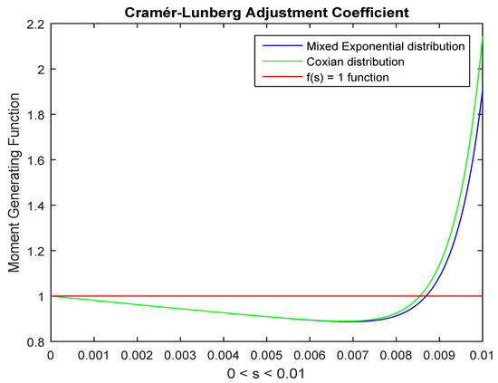
Figure 1.
Graphical solution for the adjustment coefficient.
Table 1 shows that the adjustment coefficient is much higher for hyper-exponential than Coxian distribution with the above assumptions regarding their parameters.
For Erlang distribution, increase the interest rate leads to the increase of adjustment coefficient while the inverse is observed for the time to maturity and the loan size.
For the corresponding adjustment coefficient derived from Erlang distribution for the time to default, the lower and upper constant bounds for the ruin probability are given in the following table.
Table 5 shows that the increase of the adjustment coefficient leads to the increase of the upper constant bound for the ruin probability.
Table 5.
The lower and upper bounds constant for the ruin probability.
6. Discussion
Under the Erlang distribution assumption for the default arrival process with parameter , and where , numerical simulations (Table 2 and Figure 2) show that the increase of the risk premium rate leads to the increase of the adjustment coefficient which in turn decreases the ruin probability. Conversely, when , the increase of the loan size or the time to maturity leads to the decrease of the adjustment coefficient which increases the ruin probability (Table 3 and Table 4). These results suggest that for risky clients, one may use a higher risk premium rate to reduce the risk of default. Table 1 shows that the choice of the distribution of the default arrival process influences the adjustment coefficient since the main parameter of the Coxian distribution is 100 times the parameter of the hyper-exponential (these coefficients are arbitrary chosen) distribution and the adjustment coefficient changes to . This proves that the exact distribution of the default arrival process is crucial for the accuracy of the bounds.
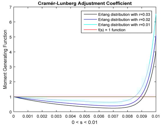
Figure 2.
Graphical solution for the adjustment coefficient.
7. Conclusions
In this paper we investigate the ruin probability in the banking sector by embedding the surplus process within the Sparre Andersen model. A general expression for the adjustment coefficient as well as the lower and upper bounds of the ruin probability are derived when the loan size is constant and the time to default follows a phase-type distribution. Special case of phase-type distributions (Erlang, Coxian and hyper-exponential) have also been investigated. Numerical results in Table 3 and Table 4 show on the one hand that the increase of the time to maturity or the loan seize leads to the decrease of the coefficient and Table 2 shows the inverse impact for the interest rate. On the other hand, Table 5 shows that the increase of the adjustment coefficient implies the increase of the upper constant bound for the ruin probability. In theory, the results of this paper can be applied to a bank. Unfortunately, due to variety of reasons, acquiring the appropriate data is a challenge within the African banking environment.
Further research still remains to be done on this subject, as: (i) on the Gerber–Shiu function which depends not only on the ruin time but also the value immediately before and after the ruin, (ii) one may consider the regime switching model to account for the risk level of the client; as a riskier client would likely pay a higher premium than a normal client. A typical model that can account for this scenario could be:
where
and is the risk rate applied for the risky client and is risk rate applied for normal client.
Author Contributions
This research paper is conducted by K.E. in the framework of a doctoral programme under the supervision of F.A. All authors have read and agreed to the published version of the manuscript.
Funding
This work was supported by the Global Excellence and Stature (GES) 4.0 scholarship of the University of Johannesburg.
Conflicts of Interest
The authors declare no conflict of interest.
References
- Andersen, E. Sparre. 1957. On the collective theory of risk in case of contagion between claims. Bulletin of the Institute of Mathematics and Its Applications 12: 275–79. [Google Scholar]
- Asmussen, Søren, and Tomasz Rolski. 1992. Computational methods in risk theory: A matrix-algorithmic approach. Insurance: Mathematics and Economics 10: 259–74. [Google Scholar] [CrossRef]
- Asmussen, Søren, and Mogens Bladt. 1996. Phase-type distributions and risk processes with state-dependent premiums. Scandinavian Actuarial Journal 1996: 19–36. [Google Scholar] [CrossRef]
- Asmussen, Søren, Florin Avram, and Martijn R. Pistorius. 2004. Russian and American put options under exponential phase-type Lévy models. Stochastic Processes and Their Applications 109: 79–111. [Google Scholar] [CrossRef]
- Bladt, Mogens. 2005. A review on phase-type distributions and their use in risk theory. ASTIN Bulletin: The Journal of the IAA 35: 145–61. [Google Scholar] [CrossRef]
- Burnecki, Krzysztof, Paweł Miśta, and Aleksander Weron. 2005. Ruin Probabilities in Finite and Infinite Time. In Statistical Tools for Finance and Insurance. Berlin/Heidelberg: Springer, pp. 341–79. [Google Scholar] [CrossRef]
- Bühlmann, Hans. 2007. Mathematical Methods in Risk Theory. Berlin: Springer Science & Business Media, vol. 172. [Google Scholar]
- Buchholz, Peter, Jan Kriege, and Iryna Felko. 2014. Input Modeling with Phase-Type Distributions and Markov Models: Theory and Applications. Berlin: Springer. [Google Scholar]
- Cody, Donald D. 1988. Probabilistic Concepts in Measurement of Asset Adequacy. Transactions of Society of Actuaries 40: 149–172. [Google Scholar]
- Cramér, Harald. 1926. Review of F. Lundberg’s “Försäkringsteknisk riskutjämning”. Skand. Aktuarietidskr 9: 223–45. [Google Scholar]
- Cramér, Harald. 1930. On the Mathematical Theory of Risk. Försäkringsaktiebolaget Skandias Festskrift. Stockholm: Centraltryckeriet, pp. 7–84. [Google Scholar]
- Dickson, David. 1994. An Upper Bound for the Probability of Ultimate Ruin. Scandinavian Actuarial Journal 1994: 131–38. [Google Scholar] [CrossRef]
- Egami, Masahiko, and Kazutoshi Yamazaki. 2014. Phase-type fitting of scale functions for spectrally negative Lévy processes. Journal of Computational and Applied Mathematics 264: 1–22. [Google Scholar] [CrossRef]
- Gerber, Hans U. 1979. An Introduction to Mathematical Risk Theory. Number 517/G36i. Philadelphia: S. S. Huebner Foundation for Insurance Education. [Google Scholar]
- Grandell, Jan. 1991. Aspects of Risk Theory. New York: Springer. [Google Scholar]
- Kolb, Robert W., Gerald D. Gay, and William C. Hunter. 1985. Liquidity requirements for financial futures investments. Financial Analysts Journal 41: 60–68. [Google Scholar] [CrossRef]
- Longstaff, Francis A. 2010. The subprime credit crisis and contagion in financial markets. Journal of Financial Economics 97: 436–50. [Google Scholar] [CrossRef]
- Lundberg, Fillip. 1903. Approximerad framställning av sannolikhetsfunktionen. aterförsäkring av kollektivrisker. Akad. Ph.D. thesis, Afhandling. Almqvist och Wiksell, Uppsala, Sweden. [Google Scholar]
- Lundberg, Fillip. 1909. Uber die Theorie der Ruck-versicherung. Transactions of the VIth International Congress of Actuaries 1: 877–948. [Google Scholar]
- Mohan, Rakesh. 2009. Global Financial Crisis: Causes, Impact, Policy Responses and Lessons. Mumbai: Reserve Bank of India Bulletin, pp. 879–904. [Google Scholar]
- Nkusu, Mrs Mwanza. 2011. Nonperforming Loans and Macrofinancial Vulnerabilities in Advanced Economies. Number 11-161. Washington: International Monetary Fund. [Google Scholar]
- Neuts, Marcel F. 1975. Probability distributions of phase type. In Liber Amicorum Prof. Emeritus H. Florin. Louvain-la-Neuve: Department of Mathematics, University of Louvain, pp. 173–206. [Google Scholar]
- Neuts, Marcel F. 1981. Matrix-Geometric Solutions in Stochastic Models: An Algorithmic Approach. Baltimore: Johns Hopkins University Press. [Google Scholar]
- Quaigrain, Rita Ansah. 2013. Ruin Probabilities for Stochastic Flows of Financial Contracts. Master’s thesis, Stockholms Universitet, Stockholm, Sweden. [Google Scholar]
- Ramsay, Colin M. 2003. A solution to the ruin problem for Pareto distributions. Insurance: Mathematics and Economics 33: 109–16. [Google Scholar] [CrossRef]
- Rolski, Tomasz, Hanspeter Schmidli, Volker Schmidt, and Jozef Teugels. 1998. Stochastic Processes for Insurance and Finance. Hoboken: John Wiley & Sons, vol. 505. [Google Scholar]
- Wei, Li, and Hai-liang Yang. 2004. Explicit expressions for the ruin probabilities of Erlang risk processes with Pareto individual claim distributions. Acta Mathematicae Applicatae Sinica 20: 495–506. [Google Scholar] [CrossRef]
- Yamazaki, Kazutoshi. 2017. Phase-type approximation of the gerber-shiu function. Journal of the Operations Research Society of Japan 60: 337–52. [Google Scholar] [CrossRef][Green Version]
© 2020 by the authors. Licensee MDPI, Basel, Switzerland. This article is an open access article distributed under the terms and conditions of the Creative Commons Attribution (CC BY) license (http://creativecommons.org/licenses/by/4.0/).