Testing the Least-Squares Monte Carlo Method for the Evaluation of Capital Requirements in Life Insurance

Abstract

In this paper, we test the efficiency of least-squares Monte Carlo method to estimate capital requirements in life insurance. We choose a simplified Gaussian evaluation framework where closed-form formulas are available and allow us to obtain solid benchmarks. Extensive numerical experiments were conducted by considering different combinations of simulation runs and basis functions, and the corresponding results are illustrated.

1. Introduction

Evaluating capital requirements in a proper way is of primary importance to construct an efficient risk management system in life insurance business. In Europe, the Solvency II directive prescribes that insurers must hold eligible own funds at least equal to their Solvency Capital Requirements (SCR) defined as the value at risk (VaR) of the basic own funds with a confidence level of $99.5\%$ over a time horizon of one year. SCR may be computed according to the standard formula proposed by the regulator or according to a partial or full internal model developed by the insurer to better take into account specific aspects of the firm risk profile.

Evaluating VaR, defined in its most general form as the loss level that will not be exceeded with a certain confidence level during a specified period of time, is complicated by the fact that it must be computed at the risk horizon, implying that, if one tries to determine VaR according to a straightforward application of the Monte Carlo method, a nested simulation problem arises which is extremely time consuming. Instead of resorting to nested simulations, a possible alternative relies upon the least-squares Monte Carlo method (LSMC). LSMC was introduced in finance as a regression method to estimate optimal stopping times in American option pricing problems. The first contribution in this direction is due to Tilley (1993), and then generalized and extended in several ways by many authors, e.g., Carriere (1996) and Longstaff and Schwartz (2001), just to name a few.

In a life insurance context, LSMC was firstly applied by Andreatta and Corradin (2003) to evaluate the option to surrender in a portfolio of guaranteed participating policies. Since then, this technique has been applied extensively to evaluate complex riders embedded in life insurance contracts. We may mention, among others, the contributions of Bacinello et al. (2009) and Bacinello et al. (2010).

The idea of applying LSMC to determine capital requirements of insurance companies was proposed by Cathcart and Morrison (2009) and Bauer et al. (2010). Other contributions aiming at establishing the convergence of LSMC estimates together with a suitable choice of basis functions are those of Benedetti (2017) and Bauer and Ha (2013). The papers of Floryszczack et al. (2016) and Krah et al. (2018) shed light on practical implementation of LSMC to compute SCR.

In an evaluation framework described by one state variable evolving according to a geometric Brownian motion, Feng et al. (2016) conducted extensive numerical experiments to test the performance of nested simulations and LSMC techniques. To the best of the authors’ knowledge, no previous research has been conducted in a multidimensional setting to assess the efficiency of LSMC to determine capital requirements in a life insurance context. The present paper aims at filling this gap. For illustrative purposes, we restrict our attention to the stylized case where an insurer sells just one kind of policy: an equity-linked with a maturity guarantee. Moreover, we work in an extended Black–Scholes framework where two risk factors, the rate of return of a reference portfolio made up of equities of the same kind and the short interest rate, evolve according to a Gaussian model. This choice allows us to work in a context where a closed-form formula is readily available for the policy value and, as a consequence, a very accurate approximation of the insurer’s loss distribution at the risk horizon and a solid benchmark of the capital requirement can be obtained.

In the evaluation framework just depicted, LSMC can be applied by generating at first a certain number of outer simulations of the risk factors at the risk horizon. Then, a rough estimate of the insurer’s liabilities corresponding to each outer scenario is obtained by means of a very limited number of inner simulations along the remaining time horizon. Finally, by performing a least-squares regression an estimate of the insurer’s loss function is obtained and an empirical loss distribution is obtained by evaluating the estimated loss function in correspondence of the risk factors previously simulated at the risk horizon.

To test the accuracy of capital requirement estimates generated by LSMC, we conducted extensive numerical experiments by considering several combinations of the number of simulation runs combined with the number and the type of basis functions used in the regression function. By analyzing numerical results, it seems that, when policies with long duration are considered, the variability of the estimates obtained is non-negligible. The remainder of the paper is organized as follows. In Section 2 we illustrate the evaluation framework in which LSMC is applied to determine SCR. In Section 3, we illustrate the results of numerical experiments conducted to asses the efficiency of the model. In Section 4, we draw conclusions.

2. The Evaluation Framework

Preliminarily, for ease of exposition and without loss of generality, we declare that, since SCR in Solvency II is based on VaR, from now on we consider VaR and SCR as synonyms. To test the efficiency of LSMC to compute capital requirements in life insurance, we consider a simplified setting in which there is an homogeneous cohort of insured persons who buy at time $t=0$ a single premium equity-linked policy with a maturity guarantee. We do not consider mortality, hence the policy is treated as a pure financial contract.

An amount $F_0$, deducted from the single premium, is invested in a reference portfolio made up of equities of the same kind. At the maturity T, the insurer pays off the greater between the value of the reference portfolio and a minimum guarantee. We consider two different risk factors, the reference portfolio value and the short interest rate. Solvency II prescribes that SCR must be evaluated at the risk horizon, $\tau$, set equal to one year and a physical probability measure has to be used between the current date and the risk horizon while a risk-neutral market consistent probability measure has to be taken into account during the time interval from the risk horizon onward. We consider a Gaussian evaluation framework with a finite time horizon $T>0$, a probability space $(\Omega ,\mathcal{F},\mathcal{P})$, and a right-continuous filtration $IF=\{{\mathcal{F}}_t,0\le t\le T\}$ We consider a Gaussian evaluation framework where the reference portfolio value dynamics is described by

$$dF\left(t\right)=\mu F\left(t\right)dt+{\sigma }_{F}F\left(t\right)d{Z}_F\left(t\right),0\le t\le T,F\left(0\right)=F_0,$$

where $\mu$ and ${\sigma }_F$ are positive constants representing the drift and the volatility of the reference fund rate of return, and $Z_F\left(t\right)$ is a standard Brownian motion under the real-world probability measure. The short rate dynamics is described by an Ornstein–Uhlenbeck process

$$dr\left(t\right)=k(\theta -r\left(t\right))dt+{\sigma }_{r}d{Z}_r\left(t\right),0\le t\le Tr\left(0\right)=r_0,$$

where $k,\theta$, and ${\sigma }_r$ are positive constants representing the speed of mean reversion, the long-term interest rate, and the interest rate volatility, respectively, while $Z_r\left(t\right)$ is a standard Brownian motion under the real-world probability measure with correlation $\rho$ with $Z_F\left(t\right)$. We assume a complete market free of arbitrages that implies the existence of a unique risk-neutral probability measure under which the discounted price processes of all traded securities are martingales. The dynamics of the short interest rate is then described by the following stochastic differential equation

$$dr\left(t\right)=k(\overline{\theta }-r\left(t\right))dt+{\sigma }_{r}d{\tilde{Z}}_r\left(t\right),0\le t\le T,r\left(0\right)=r_0$$

where $\overline{\theta }=\theta -\lambda {\sigma }_r/k$, ($\lambda$ is the market price of the interest rate risk) and ${\tilde{Z}}_r\left(t\right)$ is a standard Brownian motion under the risk-neutral probability measure. Consequently, the dynamics of the reference fund value is

$$dF\left(t\right)=r\left(t\right)F\left(t\right)dt+{\sigma }_{F}F\left(t\right)d{\tilde{Z}}_F\left(t\right),0\le t\le T,F\left(0\right)=F_0$$

where ${\tilde{Z}}_F\left(t\right)$ is a standard Brownian motion under the risk-neutral probability measure with correlation $\rho$ with ${\tilde{Z}}_r\left(t\right)$.

The policy payoff at maturity is represented by the maximum between the reference fund value $F\left(T\right)$ and the maturity guarantee $G\left(T\right)$, and can be decomposed as the face value of a zero coupon bond $G\left(T\right)$ plus the payoff of a European call option written on the reference fund with strike price $G\left(T\right)$ and maturity T. As a consequence, the time t-value of the policy can be obtained as follows,

$$\begin{gathered} V(r_t,F_t)=E_{\mathcal{Q}}\left[e^{-{\int }_t^{T}r\left(u\right)du}(G\left(T\right)+\max (F\left(T\right)-G\left(T\right),0))\right|{\mathcal{F}}_t]= \\ =G\left(T\right)P(t,T)+C(T-t,F_t,G\left(T\right)), \end{gathered}$$

(1)

where $P(t,T)$ is the time t-value of a pure discount bond with maturity T and $C(T-t,F_t,G\left(T\right))$ is the value at time t of the European call above defined. The Gaussian evaluation setting allows us to obtain a closed-form formula for the policy value which is very useful to obtain a highly accurate estimate of SCR. In fact, in the extended Black–Scholes evaluation framework depicted above, we have $P(t,T)=\exp (\frac{1}{2}{\Sigma }_{22}-B(T-t))$ with

$$\begin{gathered} {\Sigma }_{22}=\frac{{\sigma }_r^2}{k^2}\left((T-t)-\frac{3+e^{-k(T-t)}(e^{-k(T-t)}-4)}{2k}\right), \\ B(T-t)=-\frac{1}{k}\left[\left(r_t-\frac{k\theta -{\sigma }_r\lambda }{k}\right)(e^{-k(T-t)}-1)-(k\theta -{\sigma }_r\lambda )(T-t)\right]. \end{gathered}$$

Moreover, the value of the European call option written on the reference fund with strike $G\left(T\right)$ is equal to

$$C(T-t,F_t,G\left(T\right))=F_t\Phi \left(d_1\right)-G\left(T\right)P(t,T)\Phi \left(d_2\right),$$

where $d_1=({\Sigma }_{11}+{\Sigma }_{12}-H(T-t))/\sqrt{D}$, $H(T-t)={\Sigma }_{11}/2-B(T-t)+\log (G\left(T\right)/F_t)$, $D={\Sigma }_{11}+2{\Sigma }_{12}+{\Sigma }_{22}$, ${\Sigma }_{11}={\sigma }_F(T-t)$, and

$${\Sigma }_{12}=\frac{{\sigma }_F{\sigma }_r\rho }{k}\left(\frac{e^{-k(T-t)}-1}{k}+(T-t)\right).$$

Finally, $d_2=d_1-\sqrt{D}$, and $\Phi (·)$ is the cumulative distribution function of a standard normal random variable (see Kim (2002) for the details about the derivation of $C(T-t,F_t,G\left(T\right))$).

Recalling that the insurer VaR is the maximum potential loss that can be suffered at the level of confidence $\alpha$ over the time interval $\tau$, we introduce at first the loss function at the risk horizon, defined, according to Solvency II, as the change in the insurer’s own fund along the risk horizon. For the sake of simplicity, and considering that the main difficulty in estimating the loss function distribution is relative to the liability side of the insurer’s own fund, we do not consider the change in the value of the firm’s assets, and, as a consequence, we consider as loss function $L=V(r_{\tau },F_{\tau })P(0,\tau )-V(r_0,F_0)$. While $V(r_0,F_0)$ and $P(0,\tau )$ are readily available through Equation (1), being the price of a pure discount bond and the policy value at the contract inception, respectively, to determine $V(r_{\tau },F_{\tau })$ requires great attention; indeed, it represents the policy value at the future date $\tau$ that is a random variable conditional on the realized future values of the two risk factors under the physical probability measure.

Then, VaR is defined as

$${\mathrm{VaR}}_{\alpha }=\inf \{z\in IR:F_L\left(z\right)\ge \alpha \},$$

where $F_L\left(z\right)=\mathrm{Prob}[L\le z]$ is the cumulative distribution function of the loss. A possible way to approximate its distribution is through the empirical distribution obtained by Monte Carlo simulations. This is done, at first, by generating outer simulations of the short rate and of the reference fund at the risk horizon under the physical probability measure. Then, associated with each simulated pairs of the risk factors, the policy value under the risk-neutral probability measure has to be estimated. In this particular setting, the policy value is available in closed form but, in general, it has to be computed by resorting to inner simulations of the risk factors. With the inner simulations of the risk factors at our disposal, it is possible to obtain an estimate of the policy value at the risk horizon and, as a consequence, an approximation of the loss distribution.

The problem is that this approach, based on nested simulations, is extremely time consuming. With the aim of reducing the computational complexity of the evaluation problem, the LSMC has been proposed. It consists essentially on estimating each policy value at the risk horizon by a very limited number of inner simulations. This implies that each resulting policy value can be consistently biased. Nevertheless, the loss function may be estimated by means of a least-square regression based on a set of suitably chosen basis functions.

In particular, after having generated N outer simulations of the risk factors at the risk horizon, each pair $(r_{\tau }^i,F_{\tau }^i)$ $i=1,\dots ,N$, is associated with a rough estimate $E(r_{\tau }^i,F_{\tau }^i)$ of the policy value computed through a limited number, m, of inner simulations through the time horizon $(\tau ,T]$. Hence, we have at our disposal a set ${\left\{E(r_{\tau }^i,F_{\tau }^i)\right\}}_{i=1,\dots ,N}$ which can be used to derive an approximation of the policy value $V(r_{\tau },F_{\tau })$. In fact, LSMC method assumes that the time $\tau$-policy value can be approximated as

$$V(r_{\tau },F_{\tau })\approx V_M(r_{\tau },F_{\tau })=\sum _{j=1}^M{\beta }_j{e}_j(r_{\tau },F_{\tau }),$$

(2)

where $e_j(r_{\tau },F_{\tau })$ is the jth basis function in the regression function, the ${\beta }_j$s represent the coefficients to be estimated, and M is the number of basis functions. The unknown coefficients ${\beta }_j$ can be estimated by a least-squares regression as

$$({\widehat{\beta }}_1,\dots ,{\widehat{\beta }}_M)=\underset{{\beta }_1,\dots ,{\beta }_M}{\mathrm{argmin}}\left[\sum _{i=1}^N{\left(E(r_{\tau }^i,F_{\tau }^i)-\sum _{j=1}^M{\beta }_j{e}_j(r_{\tau }^i,F_{\tau }^i)\right)}^2\right].$$

After having estimated the set $({\widehat{\beta }}_1,\dots ,{\widehat{\beta }}_M)$, we put these values in Equation (2) and obtain the approximation

$${\widehat{V}}_M^N(r_{\tau },F_{\tau })=\sum _{j=1}^M{\widehat{\beta }}_j{e}_j(r_{\tau },F_{\tau }),$$

which can be interpreted as a random variable taking on the N possible values ${\sum }_{j=1}^M{\widehat{\beta }}_j{e}_j(r_{\tau }^i,F_{\tau }^i),$ each one with probability $1/N$.

The empirical loss distribution can now be easily constructed and the requested VaR at confidence level $\alpha$ is then determined as the corresponding $\alpha N$th order statistic.

3. Numerical Results

In this section, we illustrate the results of extensive numerical experiments conducted to assess the goodness of the LSMC method in evaluating VaR of the equity-linked contract within the bivariate Gaussian model described in the previous section. All computations were performed on a custom-built workstation equipped with an Intel(R) Xeon(R) Silver 4116CPU 2.10 GHz processor with 64 GB of RAM and Windows 10 Pro for Workstation operating system. All source codes were written in R, version x64 3.6.0, R Development Core Team, Vienna, Austria.

The simulations were conducted under the physical probability measure from the contract inception up to the risk horizon. After having obtained N couples $(r_{\tau }^i,F_{\tau }^i)$, ($i=1,\dots ,N$), we associated with each couple a policy value computed by simulating, under the risk-neutral probability measure, $m=2$ paths of the risk factors from the risk horizon until the policy maturity, with the method of antithetic variates. The next step in the evaluation process is relative to the choice of the number and the type of basis functions needed to define the regression function. We considered at first an nth ($n=2,3,4,5$) degree polynomial function made up of a constant term plus all the possible monomials of order up to n that can be obtained from the two risk factors r and F. Hence, with $n=2$, the regression function is made up of six terms $(1,r,r^2,F,F^2,rF)$; with $n=3$ the regression function contains $M=10$ terms, i.e., $(1,r,r^2,r^3,F,F^2,F^3,rF,r^{2}F,r{F}^2)$; and so on. 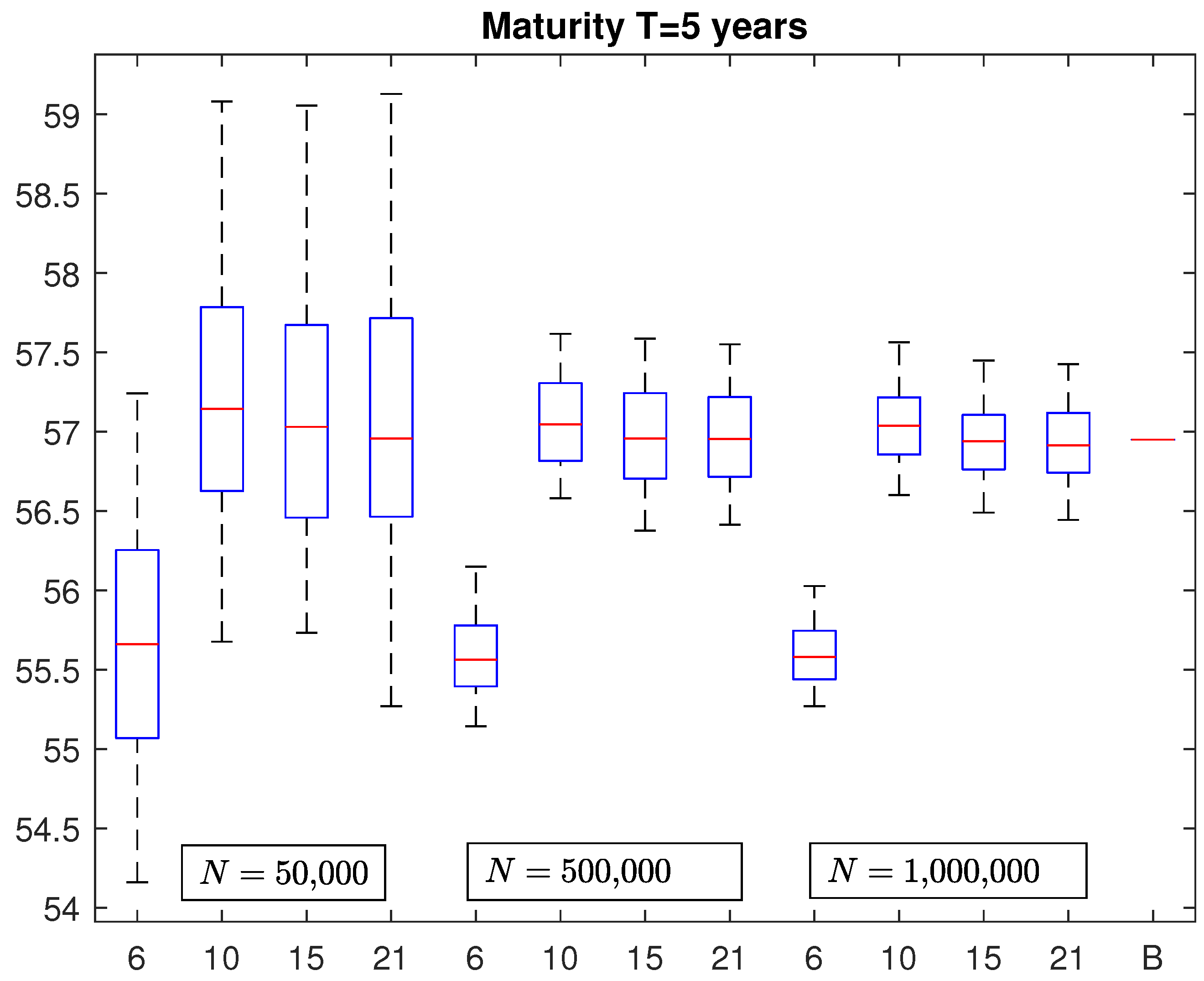For each value of n, we considered N = 50,000, 500,000, and 1,000,000 simulation runs. For the policy with maturity $T=5$ years, the corresponding results are illustrated in Figure 1. Each box plot contains 100 VaRs estimated with N = 50,000, 500,000, and 1,000,000 simulation runs, with $M=6,10,15$ and 21 basis functions, respectively. The last segment on the right, labeled B, represents the benchmark, equal to 56.9472. It has been obtained by averaging 100 VaRs, each one computed with N = 10,000,000 simulations by associating with each couple $(r_{\tau }^i,F_{\tau }^i)$ the closed-form formula of the policy value described in Equation (1), then ordering the values from the smallest to the greatest and taking the 9,950,000th-order statistic. The parameters of the stochastic processes describing the evolution of the risk factors were set equal to $\mu =0.05$, ${\sigma }_F=0.2$, $F_0=100$, $k=0.1$, $\theta =0.02$, ${\sigma }_r=0.02$, and $r_0=0.04$, while $\lambda$ and $\rho$ were set, for simplicity, equal to 0, but different values estimated on market data can be used and do not affect the precision of the evaluation model.

By looking at Figure 1, it emerges that, if we consider in the proxy function monomials of degree up to the second ($M=6$), the resulting VaRs are consistently biased regardless of the number of simulation runs considered. When we increase the number of basis functions by including monomials of Degree 3, 4 and 5, the corresponding box plots are centered around the benchmark. Moreover, the widths of the boxes reduce as the number of simulations increases. It is interesting to observe that, given the number of simulation runs, an increment in the number of basis functions from 10 to 15 and 21 does not reduce further the variability of the estimates. This is confirmed also by looking at

Table 1. This table illustrates the MAPE of VaRs computed with the LSMC method for the equity-linked policy with maturity $T=5$ years, $T=15$ years, and $T=20$ years. Each value was computed by considering a sample of 100 estimated VaRs. Four possible choices for the number of basis functions ($M=6,10,15,21$) and three possible choices of simulations runs ($N=5\times {10}^4$, $N=5\times {10}^5$, and $N={10}^6$) were considered.

	$\mathit{T}=5$ Years			$\mathit{T}=10$ Years			$\mathit{T}=20$ Years
$\mathbf{M}$\$\mathbf{N}$	$\mathbf{5}\times {\mathbf{10}}^{\mathbf{4}}$	$\mathbf{5}\times {\mathbf{10}}^{\mathbf{5}}$	${\mathbf{10}}^{\mathbf{6}}$	$\mathbf{5}\times {\mathbf{10}}^{\mathbf{4}}$	$\mathbf{5}\times {\mathbf{10}}^{\mathbf{5}}$	${\mathbf{10}}^{\mathbf{6}}$	$\mathbf{5}\times {\mathbf{10}}^{\mathbf{4}}$	$\mathbf{5}\times {\mathbf{10}}^{\mathbf{5}}$	${\mathbf{10}}^{\mathbf{6}}$
6	2.32%	2.37%	2.42%	2.74%	2.24%	2.58%	3.22%	2.35%	2.64%
10	1.21%	0.46%	0.36%	2.24%	0.70%	0.42%	4.19%	1.16%	0.93%
15	1.20%	0.48%	0.34%	2.43%	0.75%	0.47%	4.72%	1.32%	1.01%
21	1.25%	0.47%	0.35%	2.36%	0.74%	0.44%	4.22%	1.25%	0.98%

where we report the mean absolute percentage error (MAPE) of VaRs contained in each box plot. With N = 50,000, the MAPE remains above $1\%$ while for N = 500,000 and N = 1,000,000 we observe an MAPE around $0.5\%$ and $0.35\%$, respectively. Moreover, instead of simple monomials of degree n, we also considered alternative types of basis functions, such as Hermite or Legendre polynomials of the same degree, but we did not observe significant differences with respect to the results previously obtained by using simple polynomials.

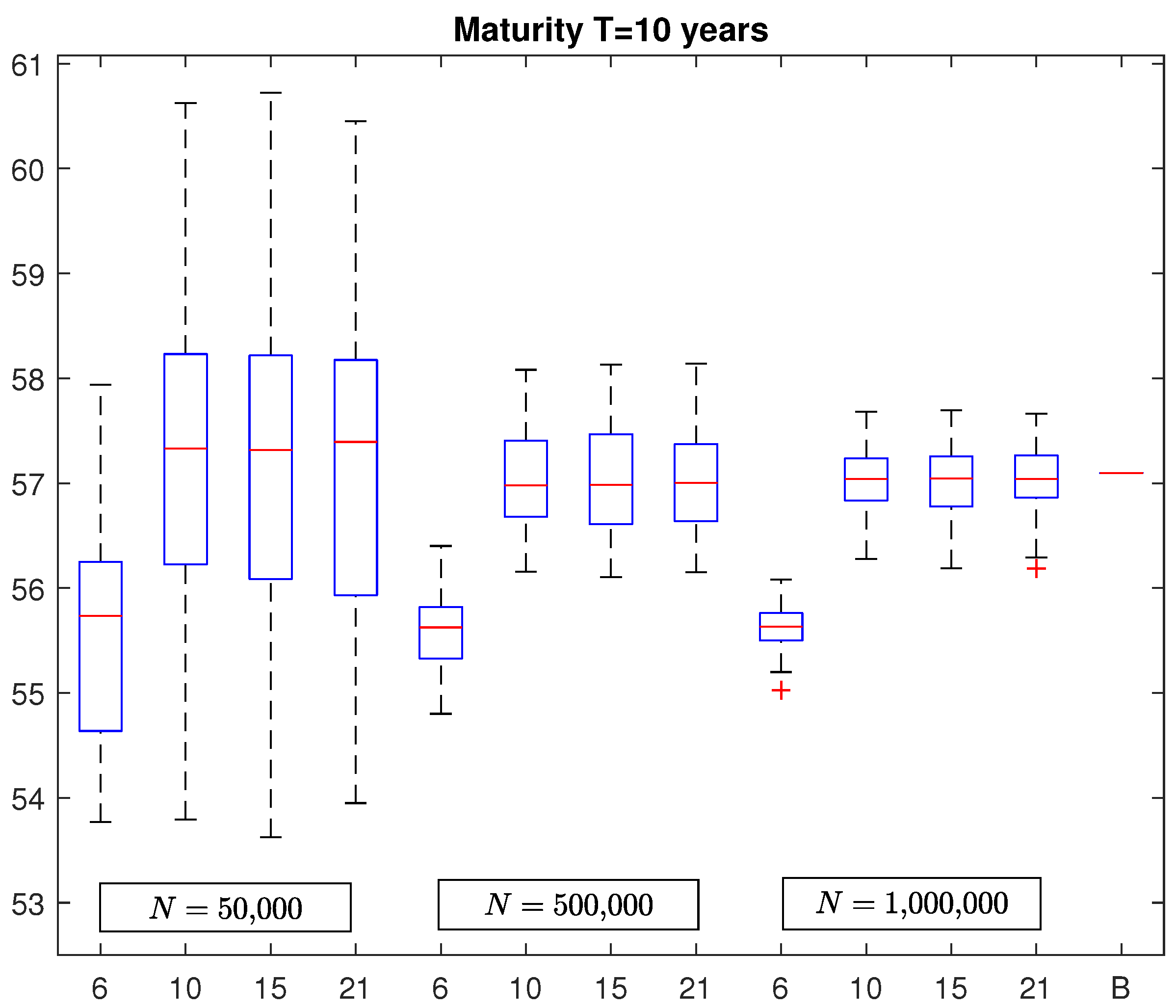
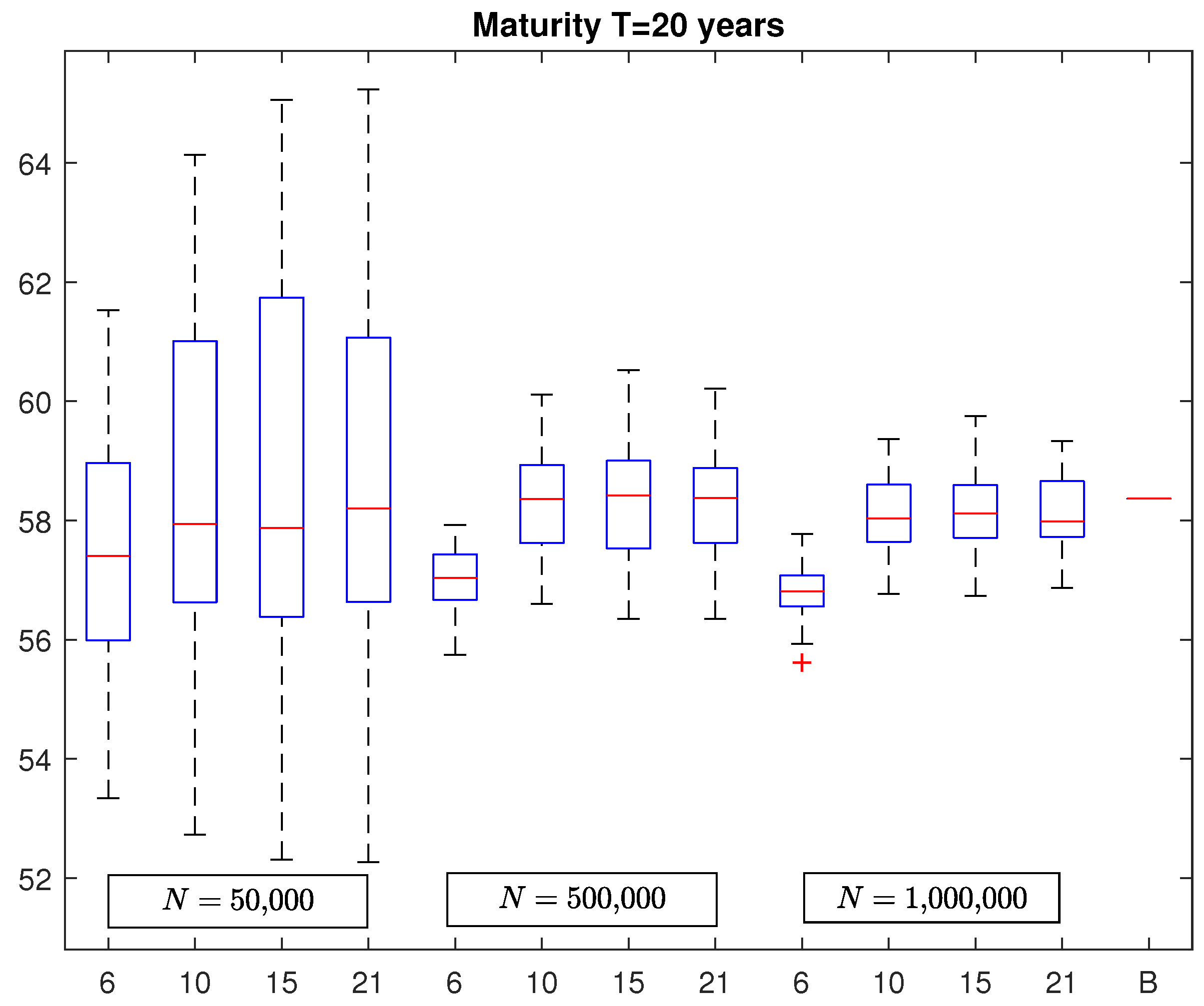
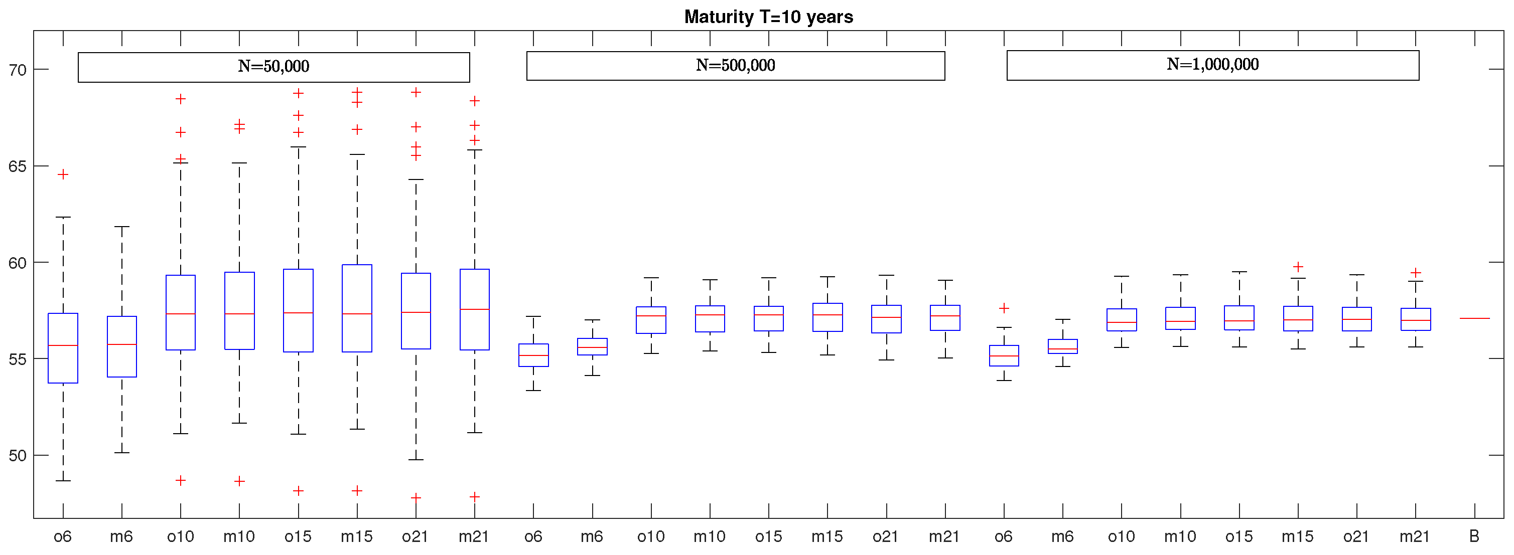
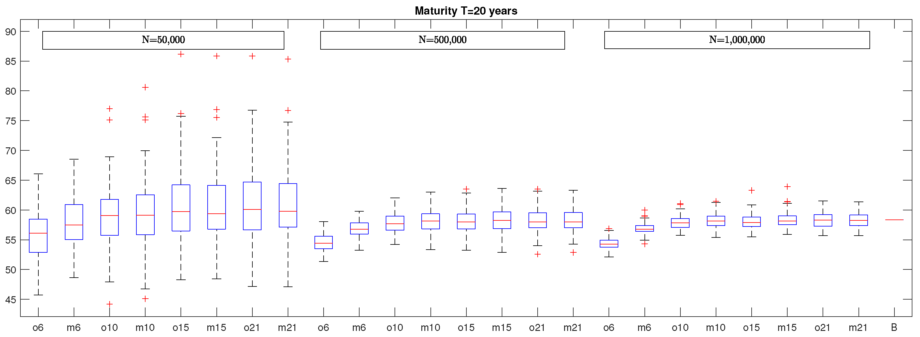
In Figure 2 and Figure 3, we report the box plots of VaR estimates in the case of a policy with maturity equal to $T=10$ and $T=20$ years, respectively. As before, the last segments represent the benchmarks which are equal to 57.1002 and 58.3666, respectively. By looking at these figures, it emerges a similar structure of the box plots already observed in the case of the five-year policy but with the obvious difference regarding to the variability of the VaR estimates that increases with the policy maturity. In fact, by considering again Table 1, we note that the MAPE increases to around $0.7\%$ and $0.5\%$ for N = 500,000 and N = 1,000,000, respectively, for the policy with maturity $T=10$ years and to $1.2\%$ and $1\%$, for N = 500,000 and N = 1,000,000, respectively, for the policy with maturity $T=20$ years. In addition, in this case, we observe no significant change in VaR estimates by considering polynomial basis functions of degree greater than 3.

It is also interesting to observe that the maximum absolute percentage error (ME) of VaR estimates in the most favorable case, i.e., when the number of simulation runs is equal to N = 1,000,000 and the number of basis functions is $M=21$, is $0.89\%$ when the maturity is $T=5$ years, $1.60\%$ when the maturity is $T=10$ years, and $2.56\%$ when the maturity is $T=20$ years.

To give an idea of the computational cost of the LSMC method compared with nested simulations, we also computed the $99.5\%$ VaR for the same policy of Table 1 with maturity $T=20$ years. As in Floryszczack et al. (2016) we considered 10,000 outer runs and 2500 inners for each outer. In

Table 2. This table reports the running times (in seconds) of the policy illustrated in Table 1 with maturity $T=20$ years. The MAPE of VaRs computed with nested simulations and the running time needed to obtain each VaR are also reported.

	$\mathit{T}=20$ Years
$\mathbf{M}$\$\mathbf{N}$	$\mathbf{5}\times {\mathbf{10}}^{\mathbf{4}}$	$\mathbf{5}\times {\mathbf{10}}^{\mathbf{5}}$	${\mathbf{10}}^{\mathbf{6}}$
6	3.54 s	34.45 s	63.76 s
10	3.83 s	34.21 s	66.17 s
15	3.68 s	33.25 s	71.84 s
21	3.60 s	31.38 s	76.89 s

Nested, MAPE = $1.09\%$ (2123.37 s).

, we report the MAPE obtained from 100 nested evaluations with the corresponding computation time (in seconds) needed to compute each VaR and the corresponding computation times for each VaR computed by LSMC with the combination of M and N of Table 1.

As shown in Table 2, the MAPE of VaRs estimated by nested simulations is similar to those obtained by LSMC with N = 1,000,000 and $M=10,15,21$. In contrast, running times of nested simulations are much higher than those needed with LSMC. Of course, it must be observed that alternative implementations of the nested simulation method are possible to obtain a better allocation of the computational budget between outer and inner simulations, but exploring such alternatives is beyond the scope of this work.

As a second experiment, we computed SCR with LSMC for the same policy considered before, but with basis functions chosen according to a different criterion. In fact, instead of using proxy functions made up of all monomials up to degree n, we considered the optimal basis functions proposed in Bauer and Ha (2013), which are those giving the best approximation of the valuation operator that maps future cash flows into the conditional expectations needed to compute capital requirements. It is shown that such optimal basis functions are represented by left singular functions of this operator, which, in the case of Gaussian transition densities, are represented by Hermite polynomials of suitably transformed state variables.1 An alternative choice of basis functions obtained according to a different optimal criterion is proposed in Feng et al. (2016). It is based, essentially, on the Hankel matrix approximation to determine optimal exponential functions. It has the advantage that the error bound can be easily controlled but it is less accurate when there is an unbounded functional relationship between response variables and dependent variables.

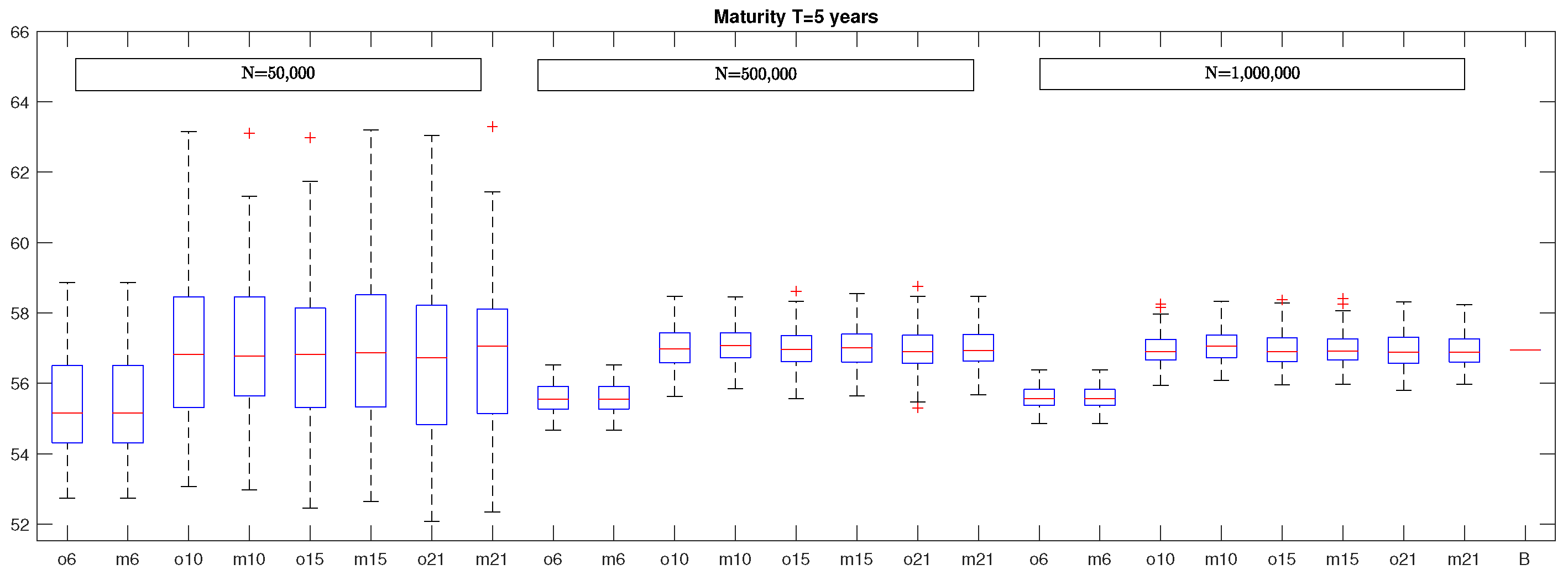
Following the approach proposed by Bauer and Ha (2013), we determined VaRs for the same policy described before but by considering optimal basis functions and we compared the results with those computed by LSMC with standard polynomials as proxy functions. In Figure 4, we report the box plots of VaR estimates computed considering different number of optimal basis functions (ox with $x=6,10,15,21$). Beside each box plot obtained through optimal basis functions the one containing VaRs obtained with simple polynomials of degree x is inserted ($mx$ with $x=6,10,15,21$), where $m6$ means that the proxy function contains all the monomials up to second degree, $m10$ means that the proxy function contains all monomials up to third degree, and so on. The eight box plots on the left were obtained by considering N = 50,000 simulation runs, the eight box plots in the middle were generated by considering N = 500,000 simulations, and the eight box plots on the right were generated with N = 1,000,000 simulations. The last segment on the right represents the benchmark.

The remaining parameters are the same as those previously considered. In all cases, each box plot was generated from 100 VaR estimates and the last segment on the right represents the benchmark. By looking at this graph, it emerges that, if we consider a number of optimal basis functions equal to six ($o6$), the resulting VaRs are biased for all the considered number of simulation runs. Similar results are obtained by considering as basis functions the six monomials up to the second degree ($m6$ in the graph). This is also confirmed by by the results in

Table 3. This table illustrates the MAPE of VaRs computed by the LSMC method with optimal basis functions in the sense of Bauer and Ha (2013) (in brackets are reported the corresponding values obtained with monomials as basis functions). Four possible choices for the number of basis functions ($M=6,10,15,21$) and three possible choices of simulations runs ($N=5\times {10}^4,5\times {10}^5$, and $N={10}^6$) were considered. Three different maturities, $T=5,10,$ and 20, years were considered. Each value was computed by considering a sample of 100 estimated VaRs.

	$\mathit{T}=5$ Years			$\mathit{T}=10$ Years			$\mathit{T}=20$ Years
$\mathbf{M}$\$\mathbf{N}$	$\mathbf{5}\times {\mathbf{10}}^{\mathbf{4}}$	$\mathbf{5}\times {\mathbf{10}}^{\mathbf{5}}$	${\mathbf{10}}^{\mathbf{6}}$	$\mathbf{5}\times {\mathbf{10}}^{\mathbf{4}}$	$\mathbf{5}\times {\mathbf{10}}^{\mathbf{5}}$	${\mathbf{10}}^{\mathbf{6}}$	$\mathbf{5}\times {\mathbf{10}}^{\mathbf{4}}$	$\mathbf{5}\times {\mathbf{10}}^{\mathbf{5}}$	${\mathbf{10}}^{\mathbf{6}}$
6	3.21%	2.41%	2.43%	4.30%	3.36%	3.35%	7.14%	6.69%	6.88%
	(3.21%)	(2.41%)	(2.43%)	(3.58%)	(2.64%)	(2.58%)	(5.92%)	(2.92%)	(2.67%)
10	2.93%	0.89%	0.69%	4.54%	1.38%	1.19%	6.88%	2.43%	1.65%
	(2.81%)	(0.85%)	(0.67%)	(4.53%)	(1.32%)	(1.14%)	(4.56%)	(2.62%)	(1.67%)
15	3.02%	0.88%	0.70%	4.77%	1.41%	1.20%	7.87%	2.68%	1.75%
	(3.13%)	(0.91%)	(0.70%)	(4.98%)	(1.48%)	(1.23%)	(8.42%)	(2.83%)	(1.77%)
21	3.42%	0.87%	0.78%	4.83%	1.49%	1.18%	8.96%	2.84%	1.93%
	(3.08%)	(0.90%)	(0.70%)	(4.77%)	(1.38%)	(1.18%)	(8.51%)	(2.74%)	(1.88%)

where we report the MAPE of VaR estimates obtained by considering optimal basis functions and the corresponding MAPE (in brackets) obtained by using standard polynomials as proxy functions. Moreover, in Table 3, we can see that, when we increase the number of optimal basis functions, the resulting estimates are centered around the benchmark with the variability that becomes smaller and smaller as the number of simulation runs is increased. It is worth noticing that MAPE does not reduce further by increasing the number of optimal basis functions to 15 and 21. This is also true when we use standard polynomials as proxy functions.

In Figure 5, we report the box plots of VaR estimates in the case of a policy maturity of 10 years, while, in Figure 6, the box plots when the maturity is 20 years are illustrated. By looking at these figures, it seems evident that the considerations already made for the policy with maturity equal to five years can be extended straightforwardly also to the cases characterized by longer maturity with the obvious caveat that the variability of VaR estimates in the different box plots increases with the policy maturity, as evidenced also in Table 1.

For what concerns the maximum absolute percentage error, we underline that the case with $M=21$ optimal basis functions and N = 1,000,000 simulations is characterized by a ME equal to $2.38\%$ for $T=5$ years, $3.94\%$ for $T=10$ years, and $5.39\%$ for $T=20$ years. If we use the same number of monomials as basis functions and the same number of simulations, we obtain a ME equal to $2.26\%$ when $T=5$ years, $4.13\%$ when $T=10$ years, and $5.11\%$ when $T=20$ years.

Another aspect to be considered is that VaR estimates obtained in this second experiment seem to be affected by a greater variability than those computed in the first experiment. This is probably due to the fact that, in the first experiment, VaRs were obtained by considering policy values at the risk horizon computed with two antithetic inner simulations, while, in the second case, VaRs were obtained, as in Bauer and Ha (2013), by considering policy values at the risk horizon computed with just one inner simulation. In general, the lack of improvement of VaR estimates when using optimal basis functions may be due to the fact that, when the dimension of the evaluation problem is low, optimal basis functions and standard polynomials may generate the same span and in this case the results are equivalent.

Moreover, based on the numerical results illustrated before, it seems that the choice of the type and of the number of basis functions is not an issue in a low-dimensional setting. In fact, with a number of simulation runs up to N = 1,000,000 a simple polynomial of degree $n=3$ gives the highest explanatory power. Since the number of basis functions represents also the rank of the matrix to be inverted in the least-squares regression, the inverse matrix can be computed almost instantaneously in these cases. Of course, given the results in Benedetti (2017), LSMC converges when the number of simulations and the number of basis functions are sent jointly to infinity; hence, increasing further the number of simulations implies that a polynomial of higher degree is needed and M will increase further too. Nevertheless, it is unlikely that in practical cases with path-dependent features a further increment in the number of simulation runs is possible, given the available computational budget, and even if this could be possible, it should be considered with great attention the possibility of devoting part of the computational budget to obtain better estimates of the insurer’s liabilities at the risk horizon eventually by increasing the number of inner simulations. This could produce a consistent improvement in the efficiency of the evaluation process. Things could be different when the number of risk factors increases considerably and it should be explored if polynomials including all possible monomials of up to a relatively low degree fit well the insurer’s loss distribution. When the dimension of the evaluation problem increases, selecting basis functions according to a certain optimal criterion will, arguably, be more useful if standard polynomials of relatively low degree will not produce accurate results. This aspect deserves further research, but, when the number of risk factors is high, numerical analyses are complicated by the fact that obtaining solid benchmarks is difficult, due to large computational burden of the evaluation problem.

4. Conclusions

We conducted extensive numerical experiments to test the efficiency of LSMC in computing capital requirements in life insurance. We considered a simple Gaussian evaluation framework where an insurer sells an equity-linked policy with maturity guarantee. This allows applying closed-form formulas to compute the policy value and, as a consequence, very accurate benchmarks were obtained. In a first stage, we considered simple monomials as basis functions. Then, we applied optimal basis functions (in the sense of Bauer and Ha (2013)) and we compared the resulting estimates with those obtained by considering standard monomials as basis functions. In the authors’ opinion, the following conclusions can be drawn:

• In the case of policy with long maturity, VaR estimates are biased even when a relevant number of simulation runs and several basis functions are used.
• The choice of the number and the type of basis functions seems not to be an issue in a low-dimensional framework as standard polynomials of degree 3 give the highest explanatory power and increasing the degree of the polynomials or using different types of basis functions do not improve the accuracy of VaR estimates.
• Further research is needed to understand if also in a high-dimensional setting polynomials of relatively low degree are able to fit well the insurer’s loss distribution. If not, basis functions obtained according to a certain optimal criterion will, arguably, be of great importance.