1. Introduction
Stochastic models for individual claims reserving were introduced roughly 30 years ago in the work of (
Arjas 1989) and (
Norberg 1993,
1999). These papers introduce the stochastic framework of marked point processes for individual claims modeling. However, they provide little guidance on statistical aspects and on the application of these models to practical problems. Surprisingly little progress has been made in using these approaches for individual claims reserving. The proposed approaches are based on (semi-) parametric models, see (
Larsen 2007;
Taylor et al. 2008;
Zhao et al. 2009;
Jessen et al. 2011;
Pigeon et al. 2013;
Antonio and Plat 2014). Unfortunately, most of these proposals turn out to have too restrictive assumptions and they are not sufficiently practical in real data applications. Individual claims reserving has only started to become popular with the emergence of machine learning methods in insurance: some papers are based on the application of regression trees and gradient boosting techniques, see (
Wüthrich 2018;
Lopez et al. 2019;
De Felice and Moriconi 2019;
Duval and Pigeon 2019;
Baudry and Robert 2019). Probably the most popular machine learning method, neural networks, has mainly been used on aggregate data, see (
Gabrielli 2020;
Kuo 2019). This seems surprising, because neural networks have gained a lot of attention in recent years due to their excellent performance on individual cases. A good introduction to neural networks and their application to insurance pricing can be found in (
Goodfellow et al. 2016;
Ferrario et al. 2018;
Denuit et al. 2019). Neural networks served at developing an individual claim history simulation machine, see (
Gabrielli and Wüthrich 2018), but these authors have not followed up on their method for the purpose of claims reserving. Moreover, (
Gabrielli and Wüthrich 2018) only model claim payments but not claim incurred because of lack of the corresponding information. Clearly, claim incurred, together with past information about the claim development process, is an important information for the prediction of future payments and should not be excluded a priori from regression models used for claim prediction.
The goal of this paper is two fold. Firstly, we would like to jointly model the development of individual claim payments and claim incurred, and secondly, we would like to explore neural networks for this task because they seem to be particularly suited for this problem. Our analysis focuses on the development of the so-called Reported But Not Settled (RBNS) claims. One can expect that the development process of individual RBNS claims could be characterized with regression models since claims reported with different features and claim histories should generate different cash flows in time and amount. Consequently, regression models for individual claims should improve reserving methods and provide more detailed information about claim developments and ultimate losses in portfolios (e.g., across segments or claim types).
In this paper, we develop regression models and postulate distributions which can be used in practice to describe the joint development process of individual claim payments and claim incurred. We apply neural networks to estimate our regression models. As regressors we use the whole claim history of incremental payments and claim incurred, as well as any feature information which is available to describe individual claims and their development characteristics. Due to a large number of regressors we would like to use in individual claim prediction, neural networks seem to be the most appropriate choice for estimating the regression functions. The fit of our regression models and distributions is tested on a real data set.
We see five contributions of this paper. The first contribution are the regression models themselves. We point out that regression models which describe the development process of claims from individual policies are fundamentally different from regression models which have been used for aggregate data. Hence, it is not possible to simply move the well-known chain-ladder type models to individual claims reserving. The second contribution is that we allow for non-Markovian dynamics of the claim development process and we test the Markovian assumption on a real data set. The standard approach in claims reserving is to only use the most recent information about the claim developments, hence, to assume a Markovian structure of the claim development process. It turns out that, in our practical example, the Markovian assumption is too strong and it is beneficial, in terms of prediction accuracy, to use the whole claim history in our regression models. Thanks to the application of neural networks, the claim history can be efficiently used for predictions of future claims. The third contribution is to jointly model incremental payments and claim incurred. From the paper by (
Quarg and Mack 2004), it is suggested that both payments and claim incurred should be used for estimating the reserve for the outstanding claim liabilities. Intuitively, the linear regression structures proposed by (
Quarg and Mack 2004) in their Munich chain-ladder model is not fully appropriate. Using the tools from neural networks, we can fit a better relation between future payments and claim incurred and past payments and claim incurred. To the best of our knowledge, there is only one paper by (
Kuo 2019) which uses neural networks with simultaneous consideration of payments and claim incurred. However, (
Kuo 2019) applies neural networks to aggregated payments and case reserves observed across all accident years and development years and multiple insurance companies. Consequently, claims from individual policies and models suited for individual claims reserving cannot be used. In (
Kuo 2019), recurrent neural networks with a mean-squared error loss function are calibrated to the whole available history of aggregated payments and case reserves. However, the non-Markovian assumption of the claim development process is not discussed in any aspect and is not validated in the paper. Moreover, there is no clear distinction in (
Kuo 2019) between random variables and their predictions, the latter typically being estimated expected values. This distinction is important, if these random variables are used as regressors in later periods. The fourth contribution of this paper is that we present a self-contained estimation procedure for our regression models and neural networks. We recommend to use the Combined Actuarial Neural Network (CANN) approach of (
Schelldorfer and Wüthrich 2019)—we suggest to use generalized linear models (GLMs), generalized additive models (GAMs) or regression trees as initial predictions, or as the initial models, from which we start training the neural networks. We use multinomial/binomial cross-entropy and Gamma loss functions for calibrations of our neural networks. These loss functions are also related to the distributions of the variables which we would like to use for predictions in the claim development process. The goal in the simulation of outstanding claims is to model not only the mean response but also the distribution of the response. This might be a real challenge in practice since simple distributions, which are common in regression problems and focus on the mean response, may not fit real data sufficiently well. We aim at correctly modeling at least the first two moments of the distribution and we focus on modeling the mean as well as the dispersion of a response with a continuous distribution. To model extreme events, we separate large claims from attritional claims and use Pareto distributions for claims above a high threshold. Finally, to the best of our knowledge this is the first paper in insurance data science where outstanding liabilities are predicted with neural networks and compared with classical chain-ladder estimates. This comparison on a real data set is the fifth contribution of this paper.
The remainder of this paper is organized as follows. In
Section 2 we introduce all claim development models. In
Section 3 we discuss the estimation procedure. The numerical example on real data set is investigated in
Section 4, and in
Section 5 we benchmark our results with the chain-ladder predictions. Finally, in
Section 6 we conclude. All calculations were done in Keras, which is an open-source API to TensorFlow.
2. Models for Individual Claims Development
Let denote the accident period of the occurrence date of an insurance claim. The accident period can be measured in days, weeks, months, quarters or years. Let denote the reporting delay after the claim occurrence date, measured in the same time units as the accident period i. Consequently, denotes the reporting period (in days, weeks, months, quarters or years) of a particular claim. After a claim is reported, it develops over its settlement time. Let measure the development periods of a reported claim, initialized to the respective reporting date .
We investigate individual claims from individual insurance policies. Let
denote the
incremental payment in development period
k for a claim of accident period
i reported with delay
j. The payment
is made in calendar period
. Let
denote the
claim incurred at the end of development period
k for a claim from accident period
i reported with delay
j. The claim incurred
is observed at the end of calendar period
. We introduce the case reserve for an individual claim, which is a part of the claim incurred and corresponds to an individual claim amount estimate made by a claims adjuster. The
case reserve at the end of development period
k for a claim from accident period
i reported with delay
j is denoted by
, and it is given by
The variables should also be indexed with unique individual claim identifier (claim number), for notational convenience this index is omitted for the moment.
At the reporting date of a claim we observe the first payment and the first evaluation of the total claim incurred, i.e., we have information . Please note that can also be zero if there no payment has been made in the initial development period . Having observed the values means that the time point of the claim, reporting was fully observed and we aim at modeling the development for all later time points . Our goal is to study the development process of RBNS claims, i.e., claims for which we observed the initial state . In this paper we aim at modeling the two-dimensional process , conditionally given the initial value . Since we are interested in individual claims reserving, the two-dimensional process is modeled for each single reported claim.
Let us define a filtration
which describes the history of payments and claim incurred on an individual claim. The individual claim filtration is defined by
and it describes the history of payments and claim incurred for a claim from accident year
i and reported with delay
j. Moreover, to each individual claim we associate a vector of (static or dynamic) features, which we denote by
. E.g., the vector
may include any feature of the insurance policy such as the line of business involved, the age of the injured person, the claim type, the accident period, the reporting delay etc. The information included in the filtration
and the features
are used as regressors (explanatory variables) in our regression problems to predict
in the next development period
k.
2.1. Model 1: Occurrence of Payments and Changes in Claim Incurred
In the first step we model the indicators which indicate whether the policy generates a new payment and/or the value of the claim incurred is changed in the next development period. The severities of the incremental payments and the change in claim incurred, if needed, are modeled in the next subsections.
We define the indicator process
as follows:
and we introduce a stochastic process
, which takes values in the set
, by setting:
To model occurrences of payments and changes in claim incurred, we have to model the conditional probabilities for the sequence of random variables . We should model the conditional probabilities since we expect the categorical distribution of in development period k to depend on the individual claim history and the individual claim feature .
We use a multinomial logistic regression to model these categorical conditional probabilities as follows:
where we use three appropriate regression functions
. The regression model (
3) is called Model 1.
A presently well-understood approach is to use a generalized linear model (GLM) with a linear additive function
, or a generalized additive model (GAM) with a non-linear additive function
, and selected predictor variables from the set
. Alternatively, one can use regression trees where the best predictors from the set
are chosen as a part of the calibration and
is estimated as a piecewise constant function on subspaces defined by the predictors; in the context of individual claims reserving this was considered in (
Wüthrich 2018;
Lopez et al. 2019;
De Felice and Moriconi 2019;
Duval and Pigeon 2019). A more advanced approach, gaining popularity among actuaries, is to use a neural network with a non-linear non-additive function
and including all predictor variables from the set
, this was considered in (
Kuo 2019;
Gabrielli 2020), however still on aggregated claims. We aim at fitting neural networks to individual claims.
Let us recall the categorical cross-entropy loss function for a sample of size
n of independent random variables
with categorical distribution (4 categories) and estimated probabilities
, it is given by
The categorical cross-entropy loss function is closely related to the deviance loss function of the multinomial model. The deviance is equal to . We remark that minimizing the cross-entropy is equivalent to minimizing the deviance, which is performed when we fit a categorical GLM/GAM or a categorical regression tree model.
If , then we immediately know the values of the process in the next development period k, because there is not any change in claim incurred and payments are equal to zero. Therefore, we only need to further model the cases .
2.2. Models 2 and 3: Claim Severities of Incremental Payments
If
or
, we have to model a non-zero payment in development period
k for the claim under consideration. In practice, we observe both positive and negative incremental payments and we can expect that the behavior of positive and negative payments differs. By negative payments, we mean salvages and subrogations. Consequently, we can use a spliced distribution to model non-zero payments. We introduce the following sequences of random variables:
where the first sequence models positive incremental payments, given their occurrence, and the second sequence models negative recovery payments, again given their occurrence. We have to model the conditional probabilities of a positive and a negative payment together with the conditional distributions of the payments
and
, respectively. As discussed in the previous subsection, the probabilities and the distributions of
and
, respectively, in development period
k should depend on the available information included in
. The probabilities and the distributions may also depend on the change in claim incurred indicator
, since the events
or
include two different scenarios for the change in claim incurred.
The conditional probabilities of a positive or a negative payment in development period
k, respectively, given the occurrence of a non-zero payment, can be modeled with a binomial distribution. We use a binomial logistic regression model, and we set
The regression model (6) is called Model 2. The cross-entropy loss function for a sample of random variables with binomial distribution is calculated analogously to (4).
As far as distributions of
are concerned, we can expect that the payments should have a skewed distribution. It is common in actuarial practice to model claim sizes with Gamma distributions and fit Gamma regression models to claims severities. For this reason, we start with assuming that
and
have Gamma distributions where we postulate the relationships:
for an appropriate regression function
f, and
where
is called a dispersion coefficient. It was observed in many data sets, including insurance data sets, that the dispersion coefficient may not be constant. In such cases, it should be modeled with a separate regression function. A classical approach to model dispersion coefficients in GLMs/GAMs is to use a second Gamma regression model with a response directly modeling the dispersion coefficient. Consequently, we assume that
and
have Gamma distributions where we postulate the relationships:
for another regression function
. Let
denote the unscaled Pearson residual from the regression model (7) and (8). We assume that the squared residual
follows a Gamma regression with moments:
where
denotes a dispersion coefficient for the Pearson residuals. Similar assumptions are made for negative payments. The regression model (9)–(12) is called Model 3_positive, or Model 3_negative if negative payments are modeled.
We recall that the unscaled deviance loss function for a sample of
n independent random variables
with Gamma distribution with moments (9) and (10) and estimated expected values
is given by
We omit the constant 2 and use the average deviance loss function compared to the traditional definition of the Gamma deviance in GLMs/GAMs/trees. The scaled deviance loss function, which takes into account the dispersion coefficient, is given by
where
denotes the prediction from (11) and (12) for observation
.
If we combine the binomial distribution for a positive or a negative payment with the Gamma distributions for the severities of positive or negative payments, we receive the distribution of the incremental payment in development period k.
We remark that if , our modeling process is complete for period k and we can derive the values of the process in the next development period . If , we have to model the change in claim incurred at the end of the development period k which is obviously related to the payment made in development period k. If , the payment is zero but we need to consider a change in claim incurred. The next two subsections deal with changes in claim incurred.
2.3. Model 4: Closing Times
We consider the two remaining events and related to changes in claim incurred. We should differentiate between two cases: (a) the value of the claim incurred changes and the case reserve is different from zero; (b) the value of the claim incurred changes and the resulting case reserve is equal to zero. The latter is interpreted that the claim is closed at the end of period k, and we do not expect any further claim developments on that claim, unless such a claim is re-opened. Re-openings are assumed to only happen with a small probability (which still needs to be modeled). For claims that have zero case reserves at the end of period k we exactly know the change in claim incurred (i.e., in this case the severity of change in claim incurred does not need to be modeled). Therefore, it is reasonable to include an indicator for zero case reserves directly into all regression functions discussed in this section. Please note that this indicator is already included indirectly since the regression functions are assumed to depend on the whole history of paid and incurred claims from which the value of the case reserve can be derived. However, a direct inclusion will allow the neural network to learn the relevant structure more quickly.
We introduce the following sequences of random variables:
The event
is interpreted as claim closing in development period
k, given there is a change in claim incurred in the development period
k. Of course, a claim can be re-opened in the future and this is modeled through probabilities (
3). The conditional probability for the event
should depend on
, as well as on
since the events
and
include two different scenarios for payment occurrences. Finally, if a payment is made, then the value of the payment
could also have an impact on the probability of the event
.
As Model 4, we use the binomial logistic regression model described by
2.4. Model 5: Severities for Claim Incurred for Open Claims
We are left with changes in claim incurred in the non trivial scenario a) where the case reserve at the end of the development period is not equal to zero.
We introduce the sequence of random variables:
As for payments, we assume that
has a Gamma distribution with moments:
for a suitable regression function
f, and choosing another suitable regression function
Let
denote the unscaled Pearson residual from regression model (18) and (19). We assume that the squared residual
follows a Gamma regression with moments:
The set of predictors in (18)–(21) can be deduced in a similar way as in the previous sections. The regression model (18)–(21) is called Model 5. Negative claim incurred are assigned to data errors, henceforth, they are not modeled.
Combining the results from
Section 2.2,
Section 2.3 and
Section 2.4, we can model claim incurred
in development period
k and we can derive the value of the process
in the next development period
k. The modeling process for the next development period is complete for all scenarios of potential claims developments.
2.5. Large Incremental Payments and Claim Incurred in Models 3 and 5
Typically, general insurance claims are skewed and heavy tailed. A traditional approach in actuarial pricing and reserving is to separate large claims from attritional claims. Large claims are usually identified by using techniques from Extreme Value Theory (EVT), and claims above a high threshold are modeled with Pareto distributions. In our case, we should model large incremental payments and large changes in claim incurred in each development period By a large claim we understand a large incremental payment in Models 3 or a large change in claim incurred in Model 5.
Let
denote a threshold and
denote a positive incremental payment in development period
k. We postulate a Pareto tail
where
is called tail index. A similar model can be used for large negative incremental payments and large claim incurred. In the most general claim development model, regression models should be built for the probability of a large claim and the severity of the large claim (for
and
) since claims with particular features (e.g., bodily claims) are likely to have higher propensity to generate large claims in consecutive development periods. We refrain from doing this and choose a simpler approach. In each development period
k, we set a fixed probability for the occurrence of a large claim, from which we deduce the threshold
, and estimate constant parameters
of the large claim distribution (22) using EVT. Next, based on descriptive statistics and knowledge about business, we determine key features in
which have high propensity to generate large claims and allocate large claims in simulations to claims with these features in the first place. Details are presented in
Section 4.2, below.
Consequently, we use a spliced distribution for the response in Models 3 and 5. We use a binomial distribution to decide whether the claim is attritional or large. If the claim is attritional then we use the double Gamma regression model and the Gamma distribution to predict the response, otherwise we use the Pareto distribution for the response with additional information about the features which have higher propensity to generate a large claim.
3. Estimation Approach
In this section, we explain the choices of the regression functions in our regression models (
3), (6), (9), (11), (16), (18) and (20) for the claim developments, and how they can be estimated with neural networks. A remark is also given on the estimation of large claims.
As commented in
Section 2, the vector
should include, among other features, the development period
k under consideration. Since we model development of claims over consecutive development periods
, it is natural to estimate a separate regression function for each development period
k. Hence, the regression functions
f in our regression models are index with
, and the goal is to estimate the regression function
for each
.
Alternatively, we could use development period k as an explanatory variable in the regression functions, i.e., keep the variable k in . In our numerical example we are going to use quarterly data and because developments in different quarters may have a rather different structural form, we prefer the approach of separate regression functions for each development period, because this should have fewer difficulties to cope with structural differences from one to the next period. However, if we want to model claim developments over a large number of development periods (if the business is long-tailed), then this approach will be computationally intensive and slow. Moreover, we have fewer and fewer observations available for fitting separate neural networks in each later development period. Henceforth, for all later development periods, , we fit one neural network, denoted by , where the development period k is included as a predictor in .
3.1. Initial Regression Models
Our goal is to train neural networks in the five regression models which describe the claim development process. We follow the CANN approach. We start with a simple regression model . The predictions from the simple regression model are next used as a regressor in the neural network. As initial model we choose a simple one with a few features and without interactions. The adequacy of this initial model is then validated during the training process of the neural network and other important features and interactions will be added. Usually, it should be beneficial to start training a neural network even from a simple model. Simple models can give us information about the process and reduce the loss function at the initial training step of the neural network compared to the loss function for a model generated with completely random weights.
As initial models we can use GLMs, GAMs or regression trees. GLMs are fast in estimation and providing predictions, but we have to spend more time on pre-processing the regressors as linear link functions are unlikely to hold over the whole range of the regressors. GAMs can efficiently handle non-linear relations between the response and the regressors. Consequently, the pre-processing of the regressors is less important for GAMs. However, the estimation and prediction is typically slow for GAMs. If we fit regression trees, then continuous regressors are optimally discretized and piecewise constant relations between the response and the regressors are estimated. Estimation and prediction are also fast for trees. It is hard to recommend a particular type of model as an initial model in the CANN approach. One should investigate the costs of estimation and prediction for the initial model versus the benefits from the reduction in the loss function at the initial step of training the neural network and, consequently, a lower number of epochs used in training the neural network. It may happen that we should resign from fitting an initial model and just initiate the neural network with the constant equal to the sample mean of the response (this corresponds to the initial model equal to a homogeneous model). Let us remark that in order to model the claim development process for RBNS claims, we have to fit regression models and do predictions for many development periods. Hence, the costs and benefits of different estimation strategies should be balanced.
Since the idea is to start with simple models, we can just use two predictor variables which we include in our regression functions
, for
. From the individual claim history
we only use cumulative payments defined by
and claim incurred
as predictor variables. By this choice, we assume that there is a Markovian structure in the claims development process and only the most recent information about the claim is relevant for the next step predictions, this is similar to (
Quarg and Mack 2004).
3.2. Feed-Forward Neural Networks
For each regression model considered and development period
investigated, we fit two neural networks - the so-called 0th neural network (denoted by
) and the so-called main neural network (denoted by
). For a general introduction to neural networks we refer to (
Goodfellow et al. 2016).
In 0th neural networks :
We use all predictor variables which we choose for , i.e., from we use cumulative payments and claim incurred .
As discussed in the previous section, we include the indicators and the incremental payment as regressors in the regression functions , for .
We also include the indicator . As discussed above, the status of the claim is an important predictor variable for the claim development process and we want to use it directly as a regressor in the regression functions, i.e., we guide the network more directly to the study of this variable.
As far as the vector of additional features is concerned, we include all available claims features such as accident quarter, reporting delay, claim segment, claim type and claim origin. These variables are also natural regressors whose predictive power in the claim development process we would like to test. We do not include accident year. Since claims in latter development periods come only from earlier accident years, the predictions for latter accident years in latter development periods would be based on extrapolation of the calibrated regression functions beyond the training set which we want to avoid. Moreover, we want to make the predictions based on the observed individual claim history. Yet, we include accident quarters to directly model seasonality effects. When we fit the regression function to all development periods latter than K, then also includes the development period k as a regressor.
Finally, we use the prediction from the initial model as a regressor in the neural network.
When fitting neural network , we still assume, as in , that there is a Markovian structure in the claim development process and only the most recent information about the claim is relevant for the next step prediction. However, we extend the set of predictors by using all available features of the claim, model non-linear relationships and interactions between the features. Neural network should improve the initial, simple regression model and we now fine tune the parameters of the neural network so that we result in a good neural network regression model. Comparing deviance loss functions on the same validation sets, we can test the predictive power of a simple model, where only two, potentially most important, regressors are used, versus the neural network, where more regressors are used including custom-made regressors such as the status of the claim and the indicator of a positive payment. Moreover, applying neural network , we can efficiently handle many regressors, non-linear relationships and interactions, and we should improve the predictive power of the regression model.
In main neural networks :
We use all predictor variables which we choose for ,
We add all variables included in the individual claim history as predictors in our regression models for the development period k. Hence, we relax the Markovian assumption postulated in neural network . We now assume that the whole claim development history is relevant for the prediction of the claim development process. We remark that we keep the cumulative payments in the regression functions even though the whole history is included in the regression functions. This approach is possible since neural networks do not (directly) suffer from possible collinearity effects. The reason we keep the cumulative payments in the regression functions is that we want to extend the set of predictors compared to and , i.e., we nest the models regarding the predictor variables involved. Another reason is that the calibration of a neural network may be faster if we provide feature information in the right structure.
Comparing the deviance loss functions for the 0th neural network and the main neural network on a validation set, we can verify whether the inclusion of the whole history of the claim development process improves the prediction of the payments and the claim incurred in the next development period. In other words, we can test the Markovian assumption for the development process of individual payments and claim incurred. Finally, the best neural network among and can be chosen.
3.3. Estimation of the Neural Networks
Let denote a vector of predictors which characterizes an individual observation ℓ, excluding the prediction from the initial model . In the categorical case, we model the probability that observation ℓ is in class a, for ; in the continuous case, we model the expected value of the response of observation ℓ. Let , respectively , denote the corresponding estimations from the initial model .
We train a neural network with
M hidden layers and
hidden neurons in layers
. We use standard notation for neural networks. We define the network layers:
where
denotes the (non-linear) activation function,
denotes the bias term (the constant),
denotes the network weights and
denotes a vector of predictors. For layers
, we use the hyperbolic tangent activation function for
. Finally, the mapping
gives us the prediction in the output layer
with linear activation function and the output of dimension 1.
For the Gamma regressions, we use the exponential activation function with an output of dimension 1 in layer
. We model the expected values of an individual case
ℓ by
and we shall use the log-link for the initial model (GLM or GAM) to be consistent with the exponential output activation. If the initial model is the best choice for our data set, then the fitting algorithm should choose
and
. These values are provided as initial weights for
to the fitting algorithm. The weights
are kept trainable so that the neural network can diminish the effect of the initial prediction from
on the response. The structure of the predictor in (23) can be achieved by using concatenation of two layers in Keras: the first layer contains the 1-dimensional prediction from the initial model, the second layer gives the 1-dimensional output in layer
from
M hidden layers and linear activation function in layer
.
For the categorical regressions with
classes, we use the softmax activation function with output of dimension
A in layer
. We model the (softmax) probabilities for a single case
ℓ as follows
where
denotes the reference level. As reference level
we choose, as usual, the class with the highest empirical probability. We use the logit-link for the initial model (GLM or GAM). If we stick to the initial model, we should end up with the neural network with
and
. These values are provided as initial weights for
and the weights
are trained in the fitting algorithm. The structure of the predictor in (24) can be again achieved by using concatenation of two layers in Keras: the first layer contains the
A-dimensional predictions across
A classes from the initial model, the second layer gives the
A-dimensional output in layer
from
M hidden layers and linear activation function in layer
.
Let us remark that if we resign from fitting an initial regression model , then we use a homogeneous model which means that we initiate the neural network by setting the weight , respectively the weights , equal to the logarithm of the sample mean of the response, or the sample log-odd ratios for the categorical classes.
Neural networks and for Models 1-5 are fitted by minimizing the categorical cross-entropy or the unscaled deviance loss of the regression model on a validation set. As far as fitting of double Gamma regressions in Models 3 and 5 is concerned, we use a simplified approach. We first fit a neural network or to the mean of the response assuming Gamma distribution with constant dispersion coefficient, i.e., we consider (7) and (8). Next, we calculate the Pearson residuals and we fit a second neural network or for the dispersion coefficient, i.e., we consider a second Gamma regression with constant dispersion coefficient (11) and (12). We do not iterate the estimation process as it is done when we fit double GLMs/GAMs. Even after one iteration we observe improvements in the residuals and more iterations will slow the calibration of the models.
We use drop-out probabilities as a regularization technique. To guarantee that the mean prediction is equal to the sample mean of the response, we perform the bias regularization technique proposed in (
Wüthrich 2020). For each categorical Model 1,2 and 4, we estimate a multinomial or binomial GLM with canonical link function (logit-link) where we use neurons from the last output layer estimated for the neural network as regressors in the GLM. For Gamma Models 3 and 5, we simply scale the predictions from the neural networks to obtain the correct sample mean of the response (this also includes the predictions for the dispersion coefficients and we assume that the average of the predictions for the dispersion coefficients is equal to the constant dispersion coefficient estimated with the method presented below).
The cross-entropy loss function (4) is directly available in Keras. The Gamma unscaled deviance loss function (13) is not available but can be coded as a custom loss function. Since the constant dispersion coefficient in the Gamma regression model is estimated independently of the regression function for the mean response, we can use the Gamma unscaled deviance loss when fitting neural networks in Models 3 and 5. The constant dispersion coefficient for the Gamma regression neural network is estimated with the following approach: We estimate the dispersion coefficient in the initial model using Pearson residuals and traditional estimation techniques from GLMs/GAMs. The dispersion coefficient for the neural network is estimated as the dispersion coefficient for scaled with a factor which shows an improvement in the prediction accuracy measured with the reduction in the loss functions on a validation set. This approach seems to be reasonable since drop-out probabilities and an early stopping rule are implemented, hence the number of degrees of freedom is not clear. Since the estimate of the dispersion coefficient in is based on Pearson residuals, not on deviance residuals, we use a loss function based on Pearson residuals to scale the dispersion coefficient from .
3.4. Transformations of Variables for the Neural Networks
It is known that data should be pre-processed before training a neural network. We now turn to the discussion of the pre-processing of continuous regressors and the corresponding responses, as well as to the coding schemes for categorical variables.
We advise to transform all skewed continuous predictors, except the predictions from the initial model
, by applying the logarithmic transformation:
The logarithmic transformation produces a more balanced regressor with many fewer skewed values. We do not need the logarithmic transformation when fitting GLMs/GAMs/trees, but for a unified approach, the logarithmic transformation is also applied to regressors when the GLM/GAM/tree is fitted. Moreover, the logarithmic transformation reduces the collinearity effect between cumulative payments and claim incurred. Let us remark that we do not have to apply the logarithmic transformation to predictors which are not skewed. In our numerical example the logarithmic transformation is not applied to development periods.
After the logarithmic transformation (25) is applied (if necessary), we normalize the regressors. We apply the MinMaxScaler transformation in each development period where we fit a new regression model. We note that we should not apply the MinMaxScaler transformation to skewed regressors, hence a logarithmic transformation is first required. If we directly apply the MinMaxScaler transformation to a skewed regressor, then majority of values of the transformed regressor will concentrate close to 0, as the range of a skewed regressor in the sample is likely to be very large. Taking logarithm first and next applying the MinMaxScaler transformation will give us a more balanced values in the interval .
The predictions from the initial model , treated as a regressor, are not normalized. We initiate the training algorithm by using the bias zero and attaching weight one to the prediction from the initial model and weight zero to the neural network’s output from the M-th hidden layer. If the initial predictions were normalized, we had to up-date, accordingly, the bias and the initial weight given to the initial prediction in order to start the training process of a neural network from the initial model.
The categorical regressors are coded with the one-hot encoding procedure. In our numerical example the categorical regressors can take only up to 5 levels so there is no need to use embedding layers. The categorical regressors for GLMs/GAMs/trees can be coded with standard factor procedure with dummy variables.
The responses for the Gamma regressions are scaled so that their empirical means are equal one. The scaling of the response with its sample mean is less important than pre-processing of regressors since the predictions from the initial model and the weights initialized in the training process of a neural network already set the proper scale for the response. The scaling of the response for the Gamma regression is performed in each development period where we fit a new regression model. Pearson residuals used for estimating dispersion coefficients are not scaled and the Gamma neural networks for dispersions are initiated at the point equal to the constant dispersion coefficient.
Large incremental payments and large claim incurred are removed in each development period from the training set before Gamma regression models are fitted. Pareto distributions are fitted to the large claims on the original scale.
3.5. Estimation of the Large Claims Distributions
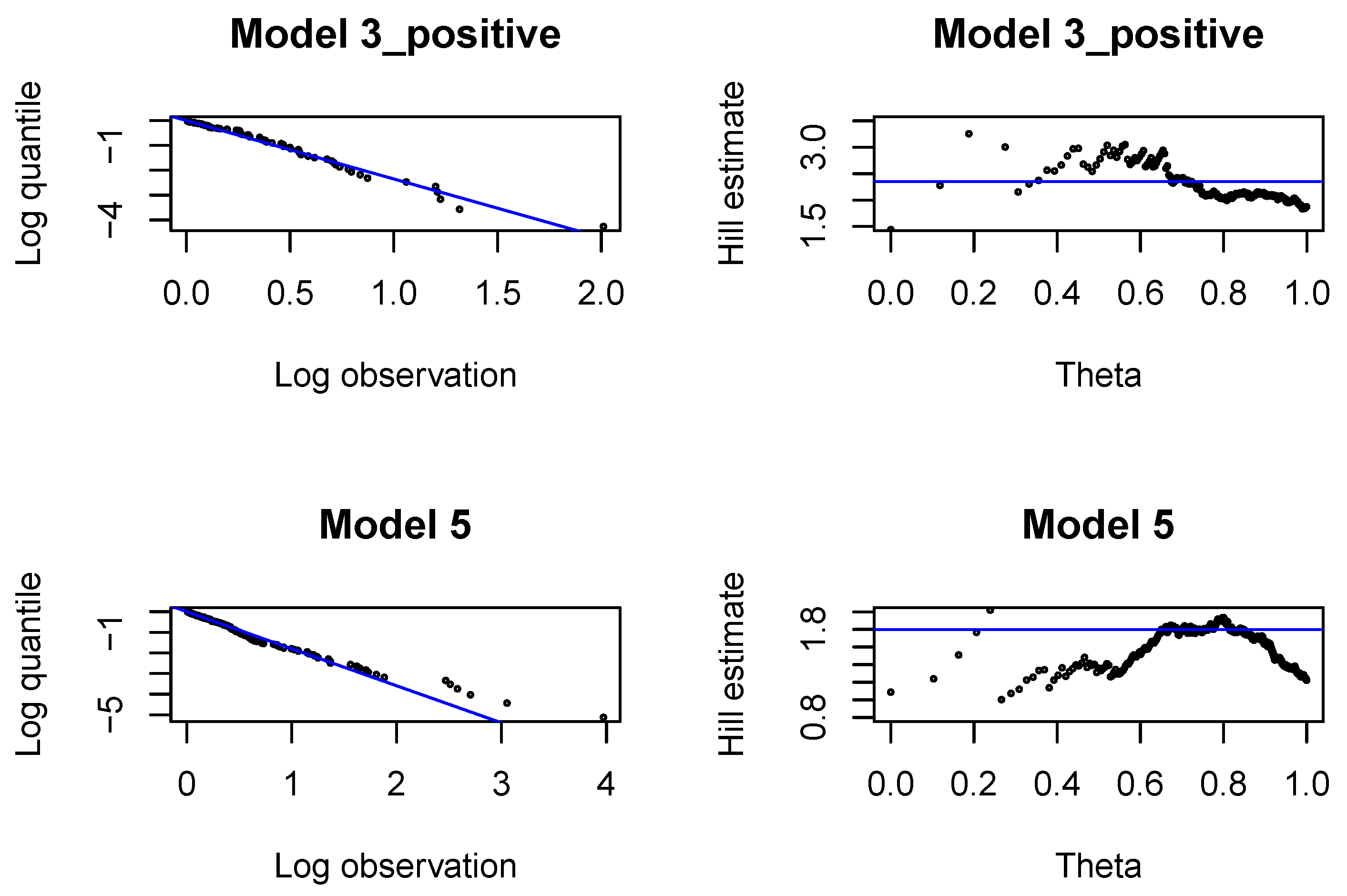
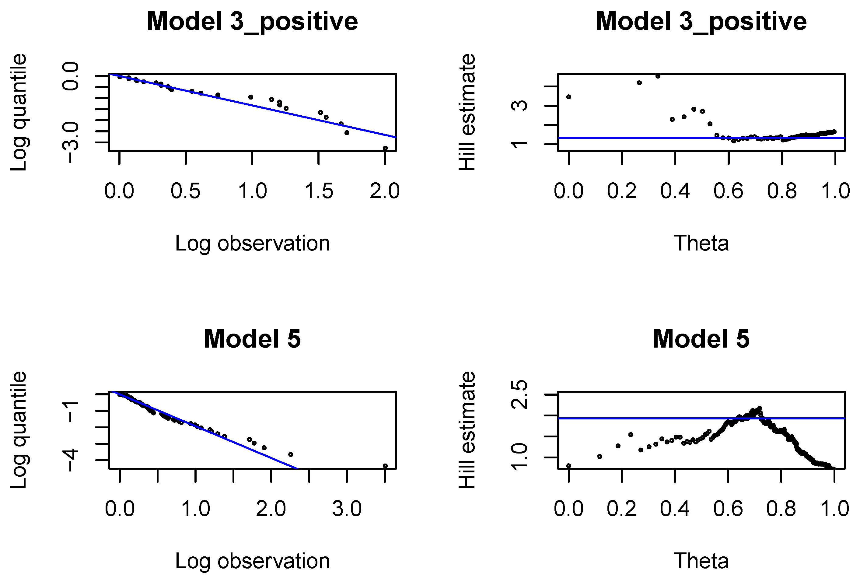
In each development period investigated, , we fit Pareto distributions to large incremental payments and large claim incurred. In each case, we identify the threshold, above which the claim is interpreted as a large claim, and estimate the tail index of large claims. The threshold and the tail index are chosen with classical methods by graphical inspection of the Pareto quantile plot and the altHill plot on the logarithmic scale. The tail index is estimated with the Hill estimator. Since we are interested in modeling large claims, we should only consider very high quantiles. The parameter of the Pareto distribution (22) is estimated with the method of moments, once is found.
Let us remark that the model for large claims is based on a conditional distribution given the claim exceeds the threshold. Hence, Models 3 and 5 should be reformulated as conditional models for attritional claims given that the claim is below the threshold. However, the deviance for truncated Gamma distribution is not tractable. Hence, we calibrate neural networks for Gamma regression models using the unconditional Gamma deviance (13). In our simulations, attritional incremental payments and attritional claim incurred generated with the Gamma regression models are truncated at the appropriate thresholds.
4. Numerical Example
In this section, we present the fitting results of our neural networks to real observations. We analyze the Markovian assumptions for the real claim development time series, the goodness-of-fit of the assumed Gamma distributions and investigate the predictive power of our neural networks in claims reserving. Supporting figures are presented in the
Appendix A. In
Section 5 we compare the ultimate payments from RBNS claims predicted with our regression models with the ultimate payments from RBNS claims predicted with the classical Chain-Ladder method.
It is known from neural network theory that one hidden layer networks are universal approximators, see (
Cybenko 1989;
Hornik et al. 1989). However, deep neural networks with multiple hidden layers may faster capture interactions between variables and better stabilize the calibration process, in general, see (
Grohs et al. 2019) for some analytical convergence results. We expect that for earlier development periods it is possible to fit deeper neural networks. However, for later development periods we have to use shallow neural networks due to the limited number of observations and increasing number of predictors related to the whole claim history. Moreover, to prevent neural networks from overfitting, we should use early stopping rules and higher drop-out probabilities if the number of calibrated parameters is large compared to the number of available observations.
4.1. Description of the Insurance Portfolio
We have a data set consisting of 1,332,495 individual claims. The data set describes the development processes of claims with accident dates and reporting dates both between January 2005 and December 2018 (the latter being called the cutoff date). It contains incremental payments and case reserves on a monthly basis for all reported claims, starting from the reporting date. We remark that a claim is included in our regression modeling in development period
k if the development of that claim in development period
k can be observed before the cutoff date of December 2018. This includes claims that were closed at an earlier date, because these claims may be re-opened. The data set also includes information about claim features. We have information about claim type (property or bodily injury), claim segment (5 segments) and claim origin (where the claim was caused—Poland or abroad). We recall that the regressors, which we use in this study, are described in
Section 3.2.
In the first step, we applied data pre-processing as follows:
We scaled incremental payments and case reserves with a constant in order to anonymize the results.
We removed the claims for which we identified inconsistencies in accident dates, reporting dates and settlement months. In a company, one should apply data cleaning to such claims by doing further investigation with involved persons.
We investigated incremental payments and case reserves. To simplify the modeling process for the purpose of the paper, we only model positive payments and resign from modeling negative payments (salvages and subrogations). Consequently, we do not fit Model 2 and Model 3_negative in this paper. For simplicity, negative payments and recoveries were set to zero in the data set.
We ended up with a cleaned data set consisting of individual claims. We removed less than of the claims from the date set. The change in the aggregate payments historically observed was , mainly caused by removal of recoveries.
The claims incurred were calculated for all claims.
For computational reasons, we fit the neural networks on quarterly data. The unit of the accident period, the reporting period and the development period is 3 months. Consequently, denotes the sum of incremental monthly payments made in the k-th quarter starting from the reporting date, and denotes the value of the claim incurred at the end of the k-th quarter starting from the reporting date (in quarterly units) for a specific claim. We deal with , since we have claims from 14 accident years in the data set.
Table 1 presents the number of observations which we can be used for fitting our regression models in consecutive development periods
. It is clear that the number of available observations decreases with the development period. This means that we are not able to estimate separate regression models for all later development periods
. We decide to fit separate neural networks for
, and one neural network for all development periods
, for each Model 1, 3_positive, 4, 5. The neural network for the last development periods is denoted as a neural network for development period
. The empirical probability that the incremental payment is zero and the claim incurred do not change (Case 0) in Model 1 in period
is
, and increases above
for later periods. We use
as a threshold probability in Model 1 for fitting separate neural networks in each development period.
In the next subsections we present the estimation results of our regression models for the selected development periods . We work with neural networks with 2 hidden layers. The rule of thumb is that the number of neurons in the first layer should be between the number of regressors and three times the number of regressors. The largest number of regressors is in Models 4 and 5, where we have 20 regressors plus regressors related to the claim history in the number of 2 times the development period considered. We investigate two choices for the number of neurons in the first layer: and . In the second layer we choose, respectively, and .
The data set is split to a training set and a validation set. We use a random split where of the observations are allocated to the training set. If we fit a categorical regression model (Model 1 or Model 4), then we use a stratified sampling and the proportions of the classes in the training set are the same as in the whole data set. In training the neural networks, we use a batch size of observations, 500 epochs for the categorical regressions, 1000 epochs for the Gamma regressions, and drop-out probabilities from to . Our experiments show that we need fewer epochs to train the categorical regressions than the Gamma regressions. We use a low learning rate at . We also test higher learning rates and we do not observe improvements in calibrations.
4.2. Predictions in Development Period
In development period
we have many observations available for fitting each regression model, see
Table 1. Moreover, the number of predictors, which we want to use in neural networks
, is small due to the short history of the claim development. Hence, we expect that we can fit deep neural networks in development period
with a large number of trainable parameters and a low drop-out probability. We choose drop-out probability at
.
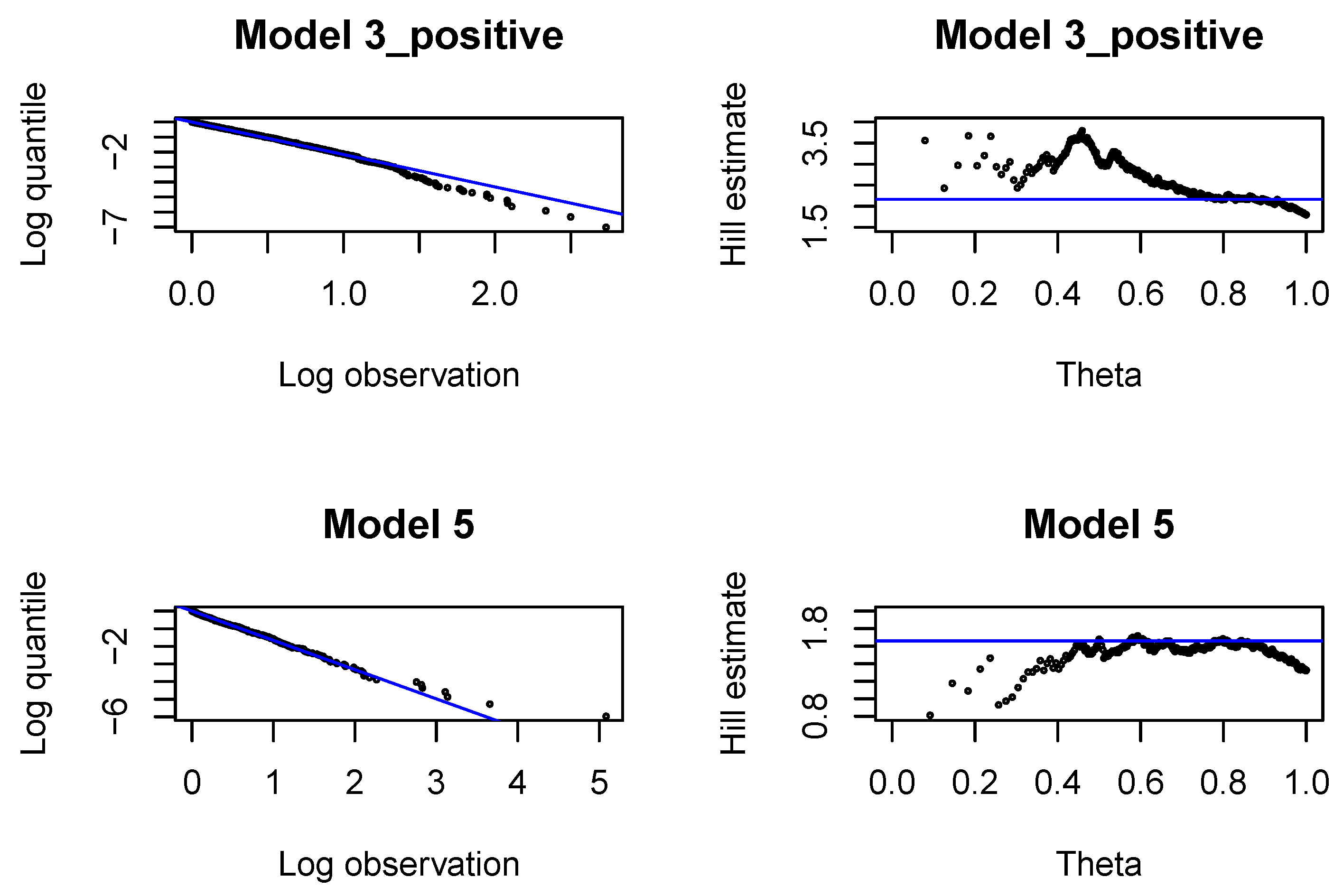
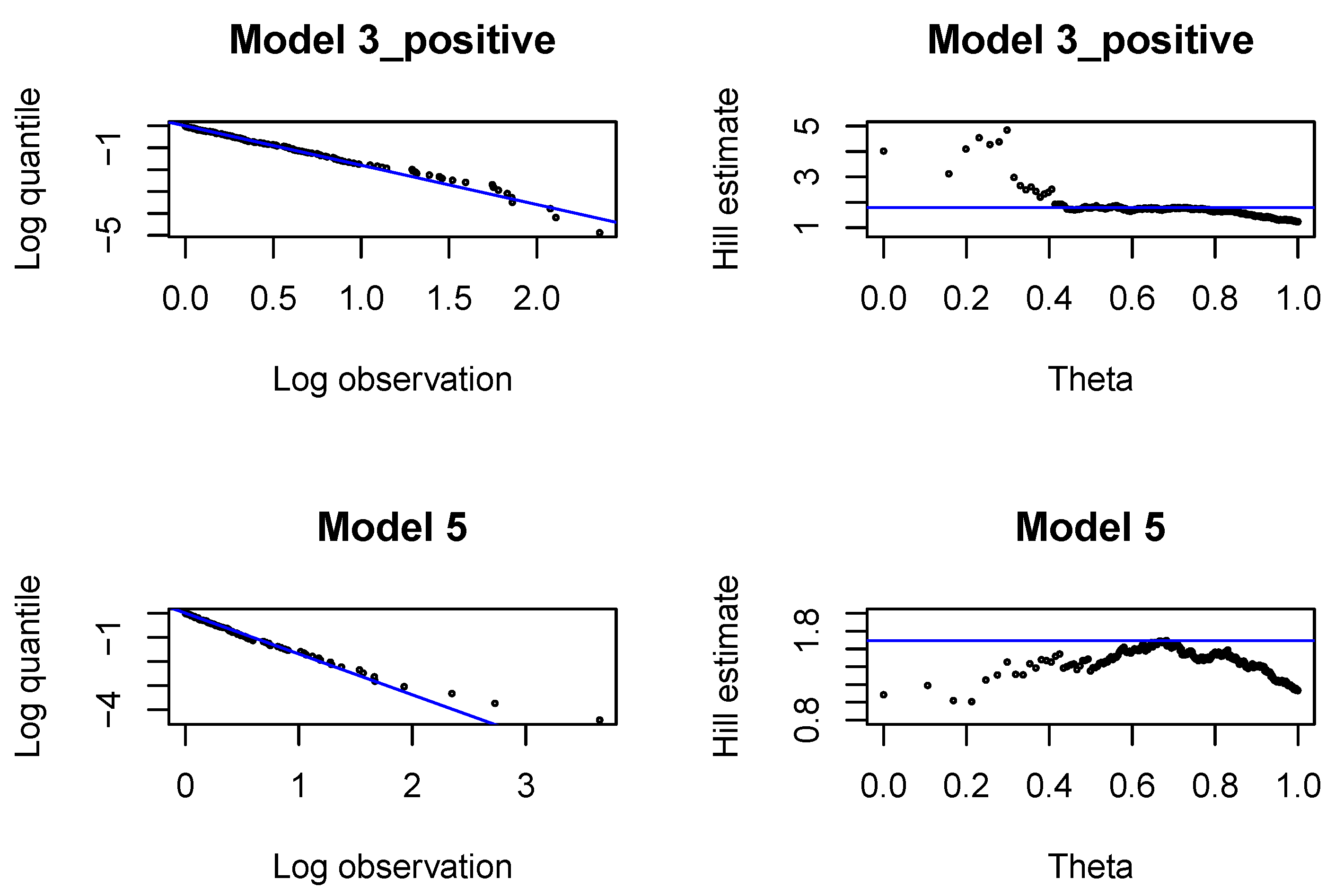
First, we analyze large claims, i.e., large incremental payments and large changes in claim incurred. We use Hill plots and we try to find the most stable region in the Hill’s estimates of the tail index, see
Figure A1. We choose the probability of a large claim at
for incremental payments and claim incurred. In
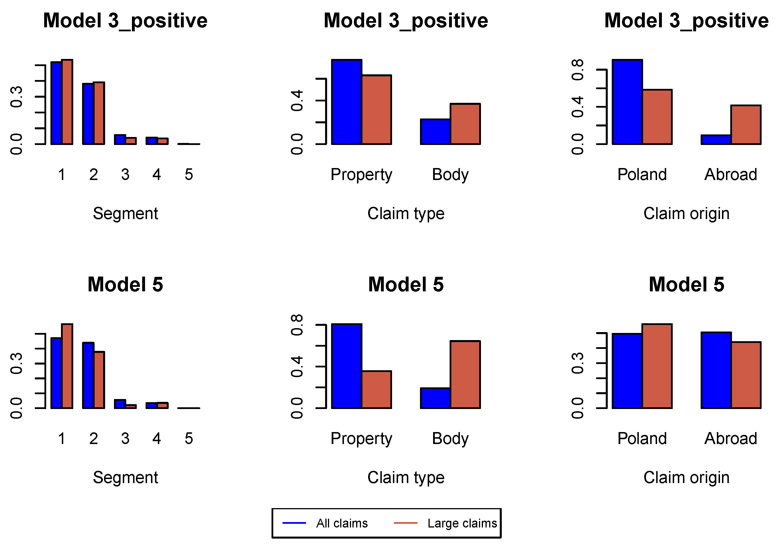
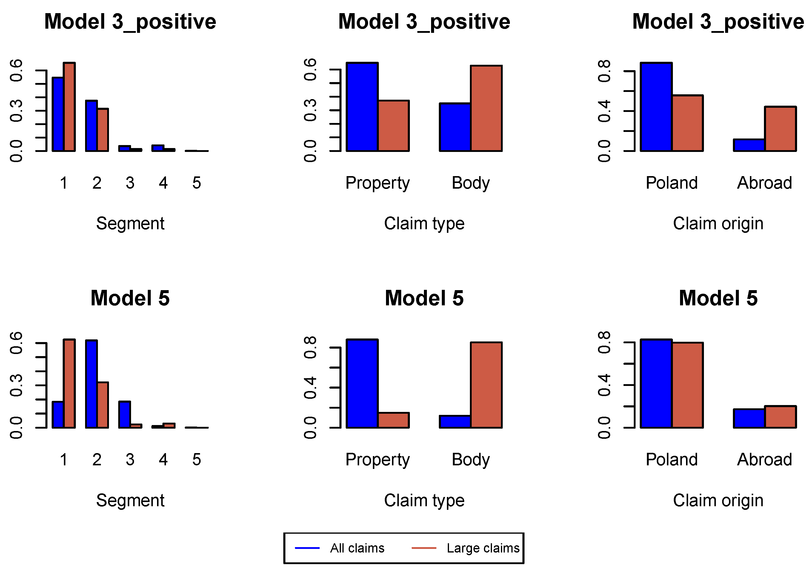
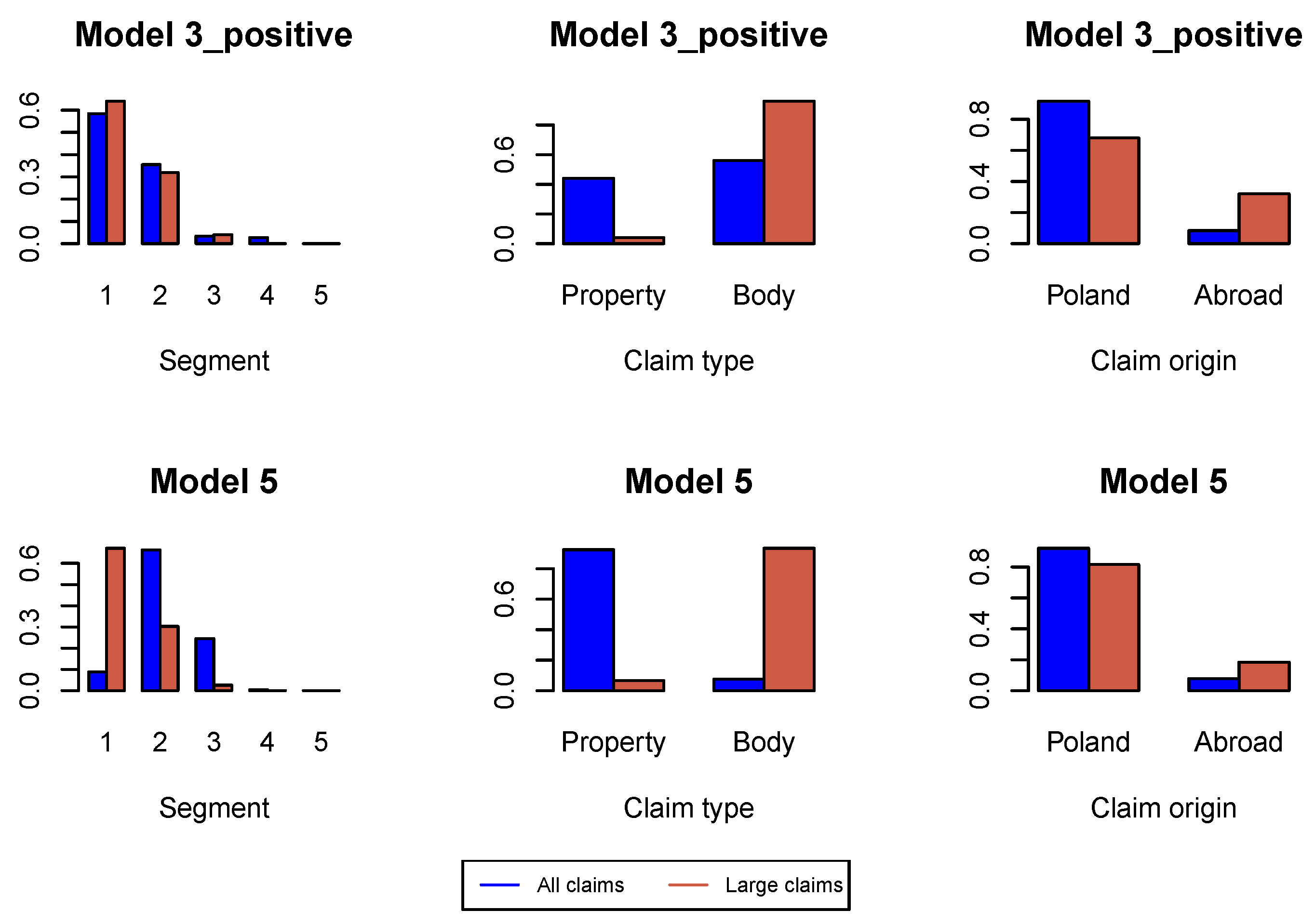
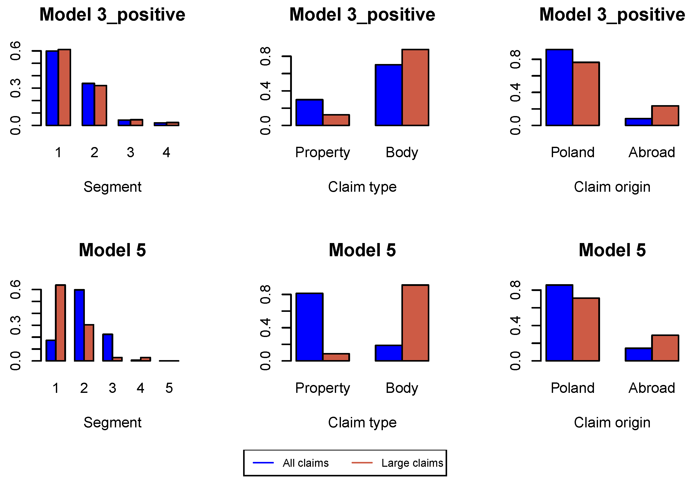
Figure A2 we study the proportions of claim features in the whole data set available for estimation of the model under investigation and in the data set consisting of large claims. We can conclude that the proportion of claims from Segment 1, bodily injury claims and claims from abroad increase in the subset of large claims. This conclusion is better pronounced in later development periods in
Figure A6,
Figure A10 and
Figure A14. Consequently, in simulations of ultimate payments, we assume that
of large incremental claims are allocated in the first place to bodily injury claims and claims from abroad, and
of large changes in claim incurred are allocated in the first place to Segment 1, bodily injury claims and claims from abroad. Remaining large claims are allocated to random claims. The proportion
is an arbitrary number.
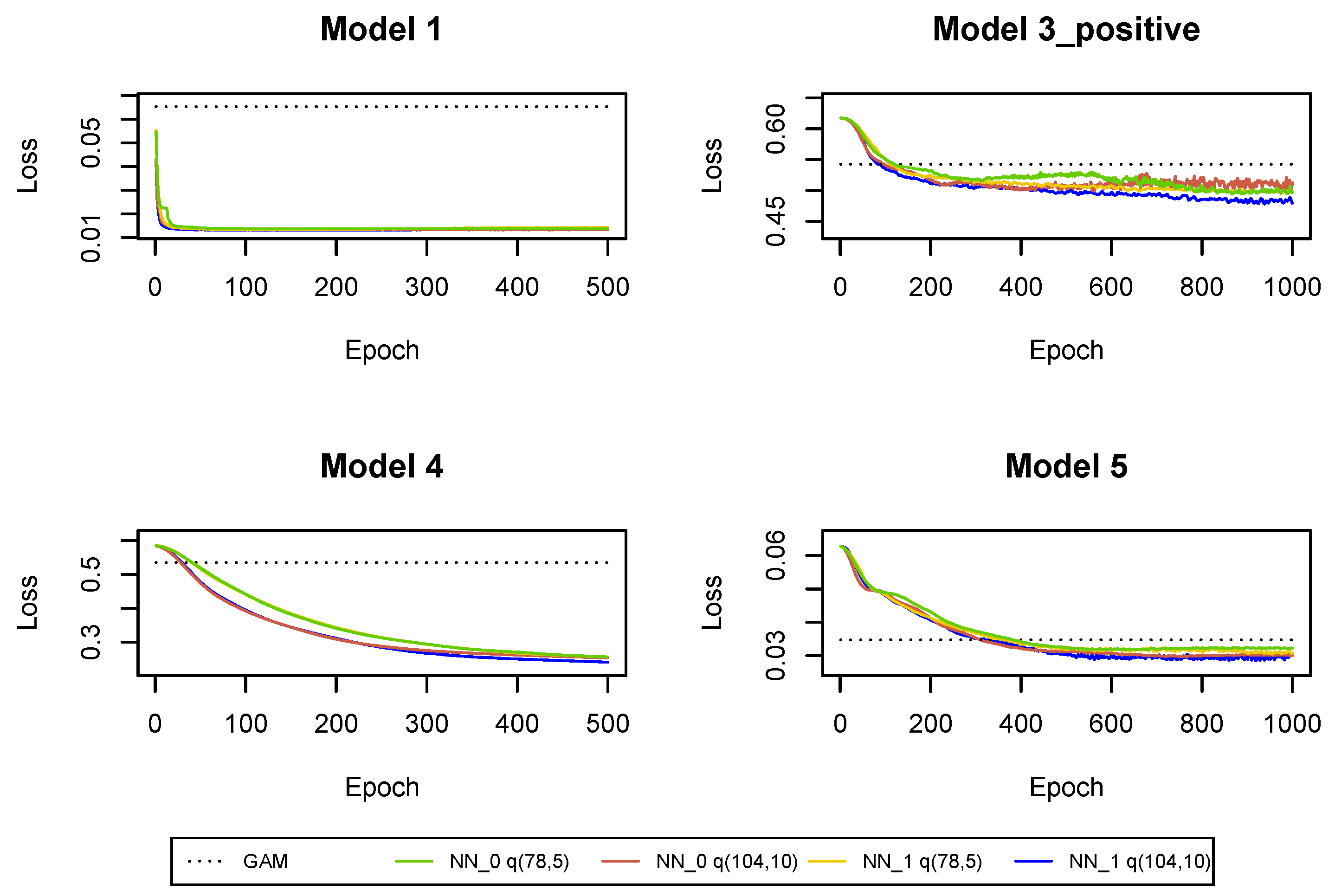
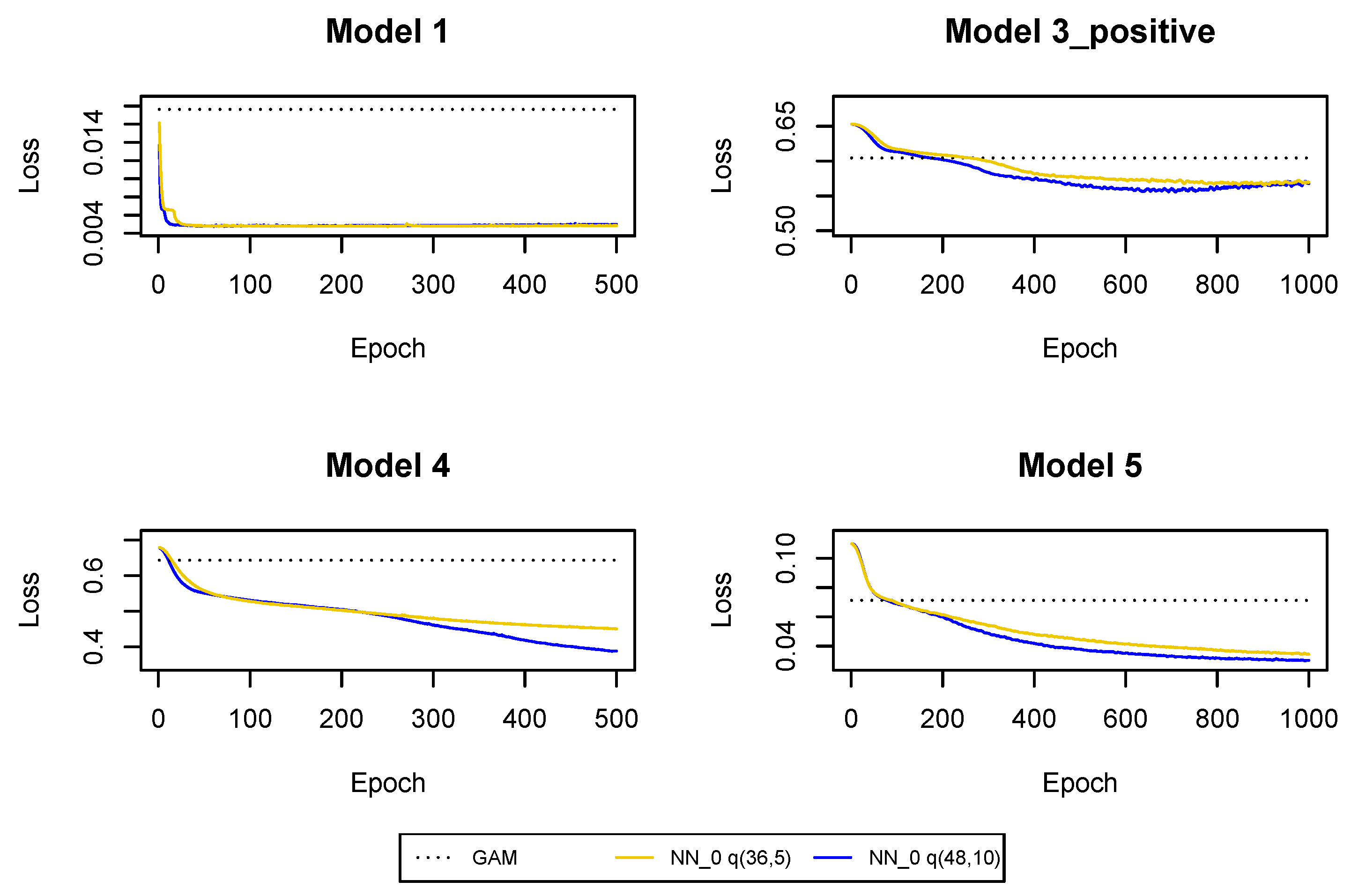
Next, we fit Models 1, 3_positive, 4, 5. We should decide which model should be chosen as an initial model from which we start training our neural networks. It turns out that GAMs and regression trees with claim incurred in the last development period and cumulative payments do not reduce significantly the loss function on the training set compared to a homogeneous model for Models 1 and 4. Hence, we decide to initiate the training of the neural networks for Models 1 and 4 starting from empirical estimates. For Models 3_positive and 5 we use regression trees with claim incurred in the last period and cumulative payments as initial models since we observe a significant decrease in the loss function on the training set compared to a homogeneous model. We initiate the training of the neural networks for Models 3_positive and 5 starting from the estimates produced by the regression tree. We could start with GAMs as and reduce the loss function at the initial training step of neural networks even more. Yet, regression trees are faster for predictions than GAMs. The disadvantage is that we have to train Gamma neural networks for more epochs.
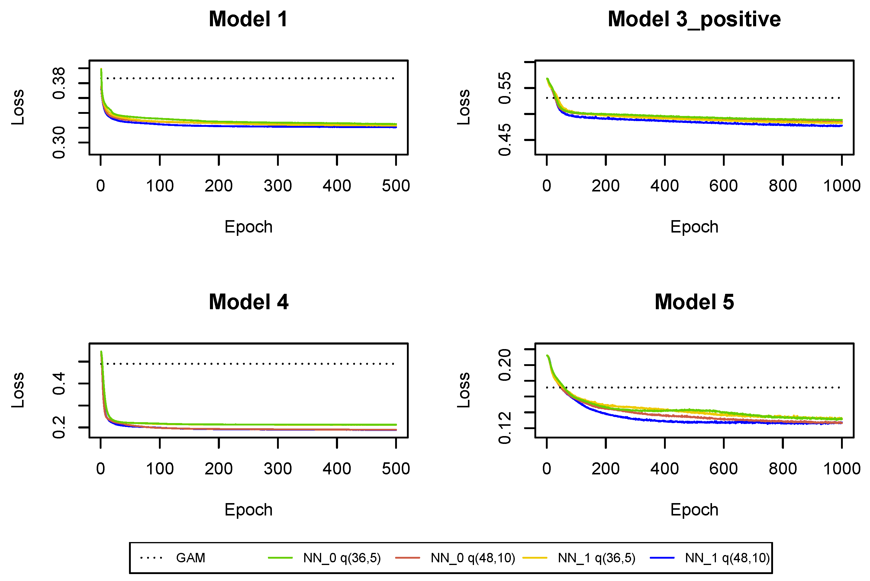
The cross-entropy and deviance loss functions on the validation sets are presented in
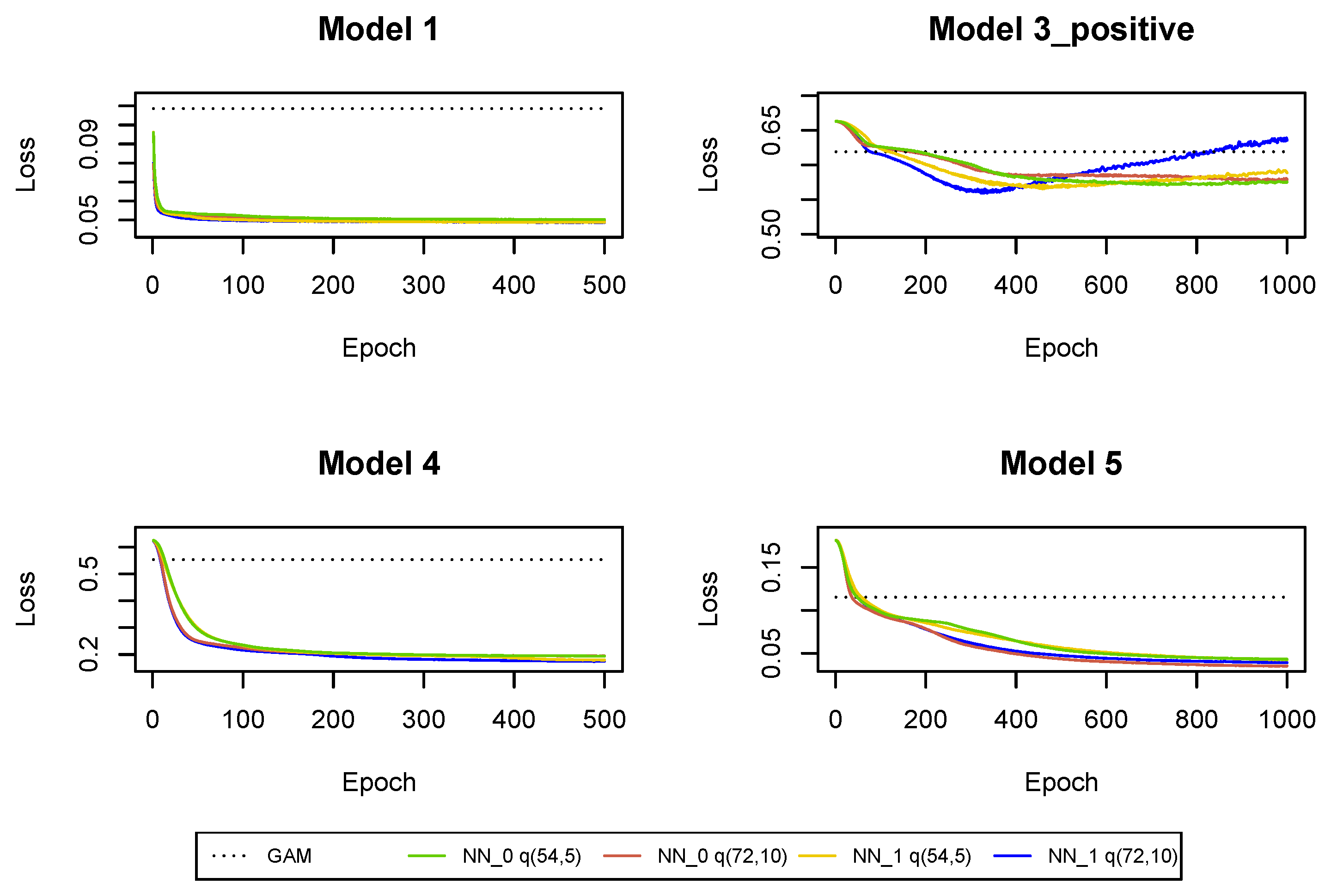
Table 2 and
Figure A3. As a benchmark, we also provide the loss functions in the GAMs where we use claim incurred in the last development period and cumulative payments as the only regressors. The predictions from
and GAM can be improved with neural networks
. We can conclude that not only the cumulative payments and the claim incurred in the last development period are useful for predictions in the next development period, but we should also use other claim features and interactions between the predictors in claims reserving. Moreover, we can observe that the use of the whole claim history also improves the predictions. Of course, for
, the use of the whole claim history means to use the two historical values of the incremental payments and the claim incurred observed in
and
. Hence, the regression models are not significantly enhanced by additional information about the claim development process. The models’ enhancement is much bigger for later development periods where, as we show in the next subsections, we should also use the whole claim history, see
Table 3 and
Table 4 and
Figure A7 and
Figure A11. It is clear that the predictions are improved in all Models 1, 3_positive, 4, 5 when we add incremental payments and claim incurred (observed in all past development periods) as regressors in the regression functions, i.e., when we switch from neural network
to neural network
. Consequently, the Markovian assumption should be rejected for the claim development processes in our data set. Finally, deeper neural networks are preferred in
since we have a large number of observations at our disposal and there is no danger that we overfit the models (by appropriately early stopping and drop-out probabilities).
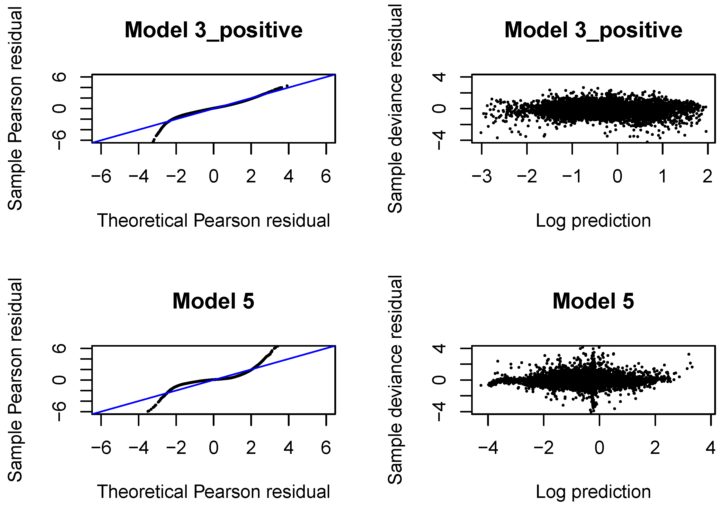
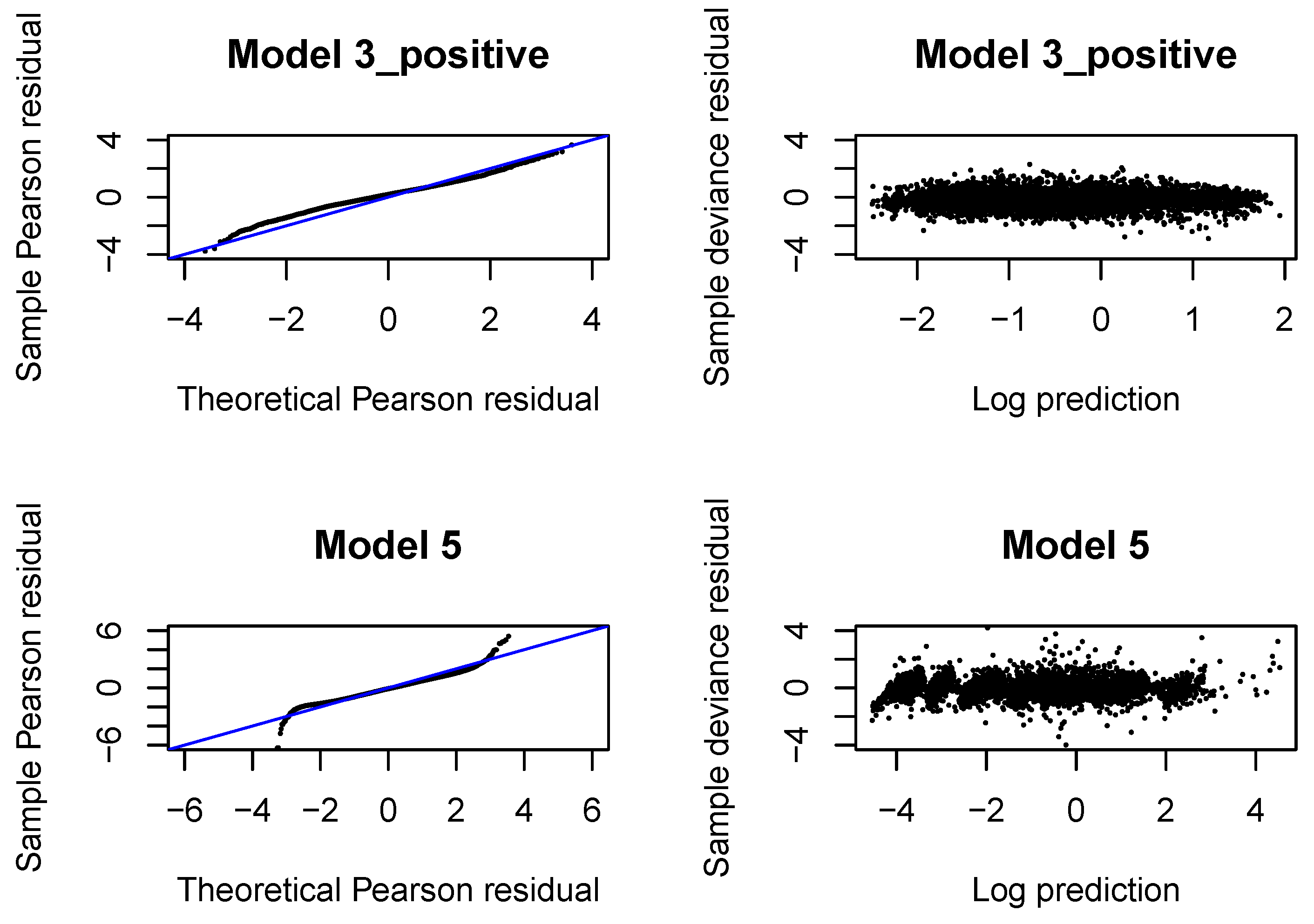
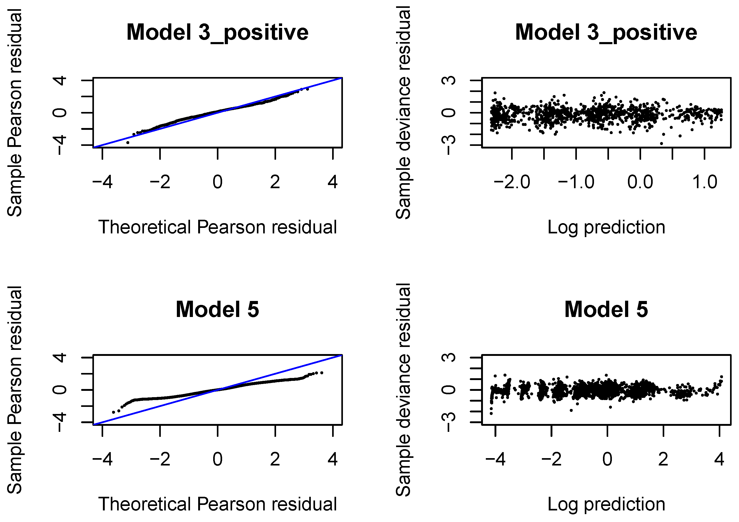
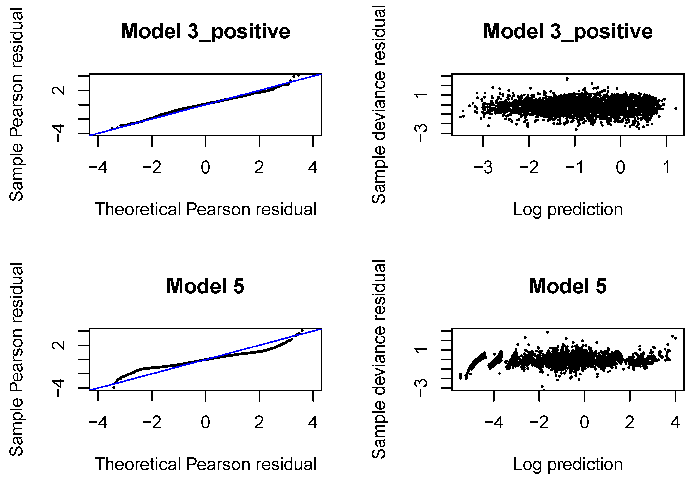
We now validate the distributional assumption that the incremental payments and the claim incurred are from Gamma distributions with the moments, respectively, given by (9)–(10), (18)–(19). As in GLMs/GAMs, we use Pearson and deviance residuals.
If the response follows Gamma distribution with true expected value and dispersion coefficient , then the Pearson residual, after adding 1, i.e., has a Gamma distribution with expected value equal to 1 and dispersion . We can use a version of a QQ normal plot to verify the Gamma distributional assumption. If denotes an observation from the Gamma distribution with true expected value equal to 1 and dispersion , in our case denotes the Pearson residual from the fitted Gamma regression model, then has a uniform distribution, where denotes the cumulative Gamma distribution function for parameters 1 and . Consequently, has a normal distribution, where denotes the inverse of the standard normal distribution function. If the Gamma distribution is the correct distribution for the response, then we should observe a straight line in the QQ-plot for the Pearson residuals from the fitted model. Let us recall that the dispersion coefficients are estimated for individual claims with the second Gamma regression model.
We also investigate the so-called Tukey-Anscombe plot where we plot the deviance residuals from the fitted Gamma regression model, scaled with the dispersion coefficients, against the log-predictions of the response in the fitted model. If the mean and variance assumptions for the distribution of the response are correct, then the deviance residuals should be fluctuate randomly around the horizontal line through zero and the deviation in the residuals should be constant.
The QQ normal plots and Tukey-Anscombe plots for the Gamma regressions fitted with
are presented in
Figure A4. We observe that the left tail is underestimated for incremental payments and both right and left tail are underestimated for claim incurred. If we look at later development periods, see
Figure A8,
Figure A12,
Figure A16, we can conclude that the Gamma distribution can be accepted for incremental payments. The choice of the Gamma distribution for claim incurred can be questioned and an improvement would be desirable. In practice, it is difficult to get a perfect fit to a Gamma distribution (with constant or varying dispersion). We should at least aim at correctly modeling the mean response and the dispersion with two neural networks. If we investigate deviance residuals, then we can conclude that the first two moments of the response are correctly modeled for incremental payments and claim incurred in all development periods. This property should be sufficient for projecting the aggregate ultimate payments in a large portfolio, estimating the best estimate and not-extreme quantiles of the aggregate ultimate payments. We would like to point out that varying dispersion improves the deviance residuals and the second neural network for the dispersion coefficient in Model 3_positive and 5 is indeed required.
4.3. Predictions in Development Period
We present the same tables and plots as in the previous section, see
Table 3 and
Figure A5,
Figure A6,
Figure A7 and
Figure A8. The conclusions are the same. We choose the probability of a large claim at
. We could differentiate the probabilities of large claims in development periods, but, if possible, we try to choose the same probability for large claims in all development periods. The drop-out probability is still set at
. We can deduce that the cumulative payments and the claim incurred in the last development period are not sufficient, except in Model 5, for precise predictions of the claim development processes. The Markovian assumption has to be rejected for the claim development processes. The fit of a Gamma distribution to incremental payments and claim incurred is acceptable. We prefer larger neural networks. Yet, the need to apply the early stopping rule, in order not to overfit Model 3_positive, can be observed in
Figure A7.
4.4. Predictions in Development Period
In development period (4 years), the set of predictors which we want to use in neural network is rather large. We want to use 51 or 52 regressors in total (where 32 regressors are related to incremental payments and claim incurred observed in the past development periods). At the same time, the number of observations is relatively small for Models 3_positive. Since the number of neurons in the first hidden layer should be at least equal to the number of regressors, the number of trainable parameters in Models 3_positive quickly approaches, and exceeds, the number of observations when we increase the number of neurons in , which we would do to improve the fit of the neural network. Consequently, the loss function may, already after a few iterations, increase on a validation set and the fitting algorithm may produce a poor prediction model. To prevent over-fitting, we can apply regularization techniques (early stopping may not be sufficient). We decide to increase the drop-out probability to get stable calibration results for Model 3_positive. We choose in . In fact, we decide to increase the drop-out probability from to for Model 3_positive starting from the development period .
We also modify the probability of a large claim in Model 3_positive. The reason is again a low number of observed payments. We choose
in development period
, and
in
. Hill plots, Pareto quantile plots and proportions of claim features in the two data sets of all claims and large claims are presented in
Figure A9 and
Figure A10.
The results of fitting neural networks for Models 1, 3_positive, 4, 5 are presented in
Table 4 and
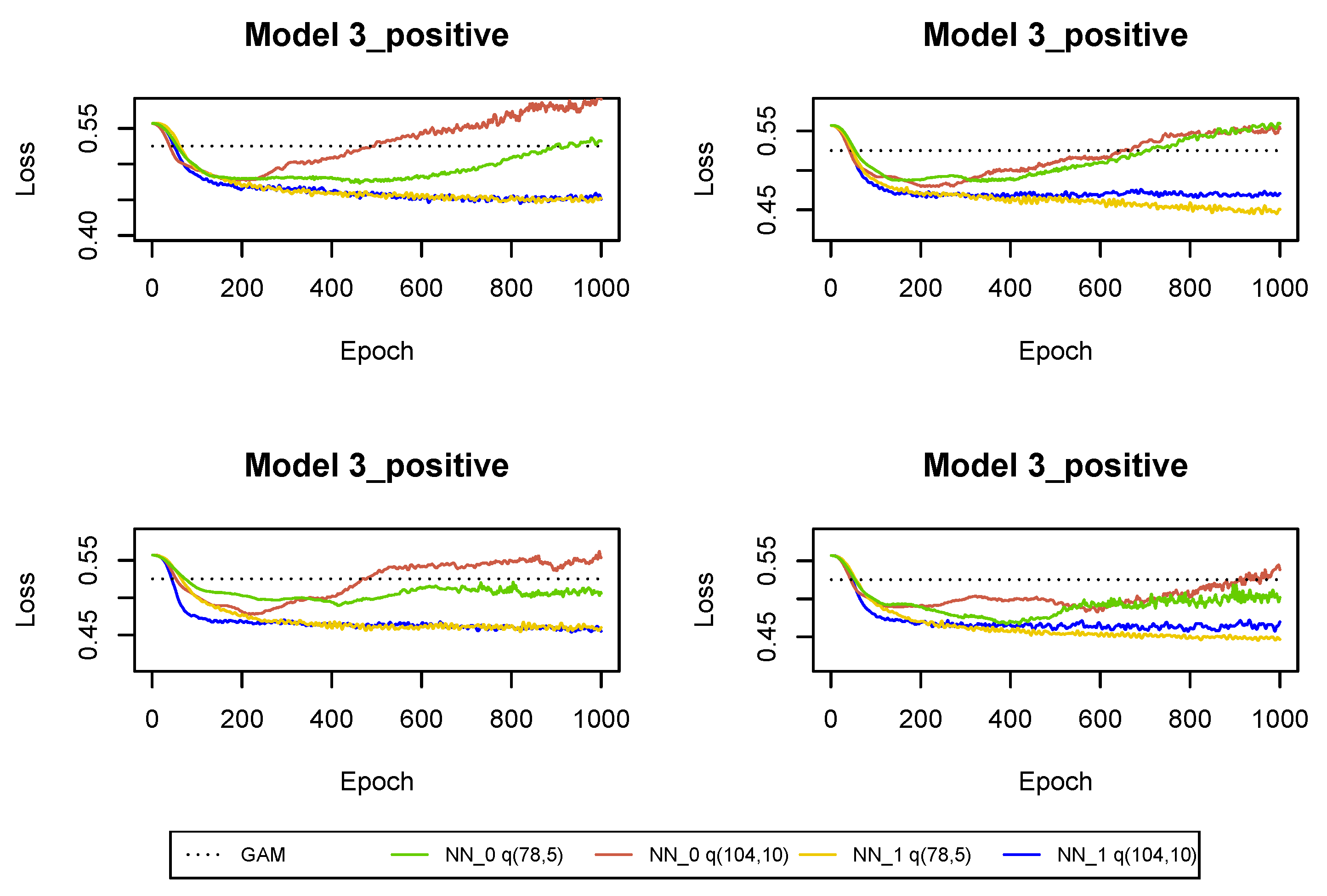
Figure A11. The conclusions are the same as in the previous sections. The larger neural network is also preferred for Model 3_positive, since it is regularized with a large drop-out probability. However, when we re-run the fitting algorithm then it turns out that in many runs the smaller network is preferred, see
Figure A17. Hence, we decide to switch to smaller neural networks for Model 3_positive starting from development period
. For Models 1, 4 an 5 we use larger neural networks in all development periods.
The residuals are presented in
Figure A12. The fit of Gamma distributions is acceptable. Yet, the estimated Gamma distribution now overestimates both tails of the claim incurred.
4.5. Predictions beyond Development Period
All claims with development periods bigger than 16 quarters are grouped into one data set and one neural network with development period information as a regressor is fitted. Due to this grouping, we cannot fit neural networks since claims in different development periods have different lengths of claim history. Hence, we fit neural network . This is justified since for latter development periods we expect that only the most recent claim history should have the greatest power in the prediction of claim development. Moreover, the results from the previous sections show that neural networks are only slightly better than in predictions on the validation sets.
Hill plots, Pareto quantile plots and proportions of claim features in two data sets of all claims and large claims are presented in
Figure A13 and
Figure A14. We choose the probability of a large incremental payment at
, and the probability of a large claim incurred at
. The probability of a large payment is higher than in the previous models. This agrees with intuition as heavier claims occur at later development periods.
The results of training the neural networks are presented in
Table 5 and
Figure A15. It is clear that
has better predictive power than
and GAM, and we prefer larger neural networks. Residuals are presented in
Figure A16. We conclude that the fit is acceptable.
Finally, in
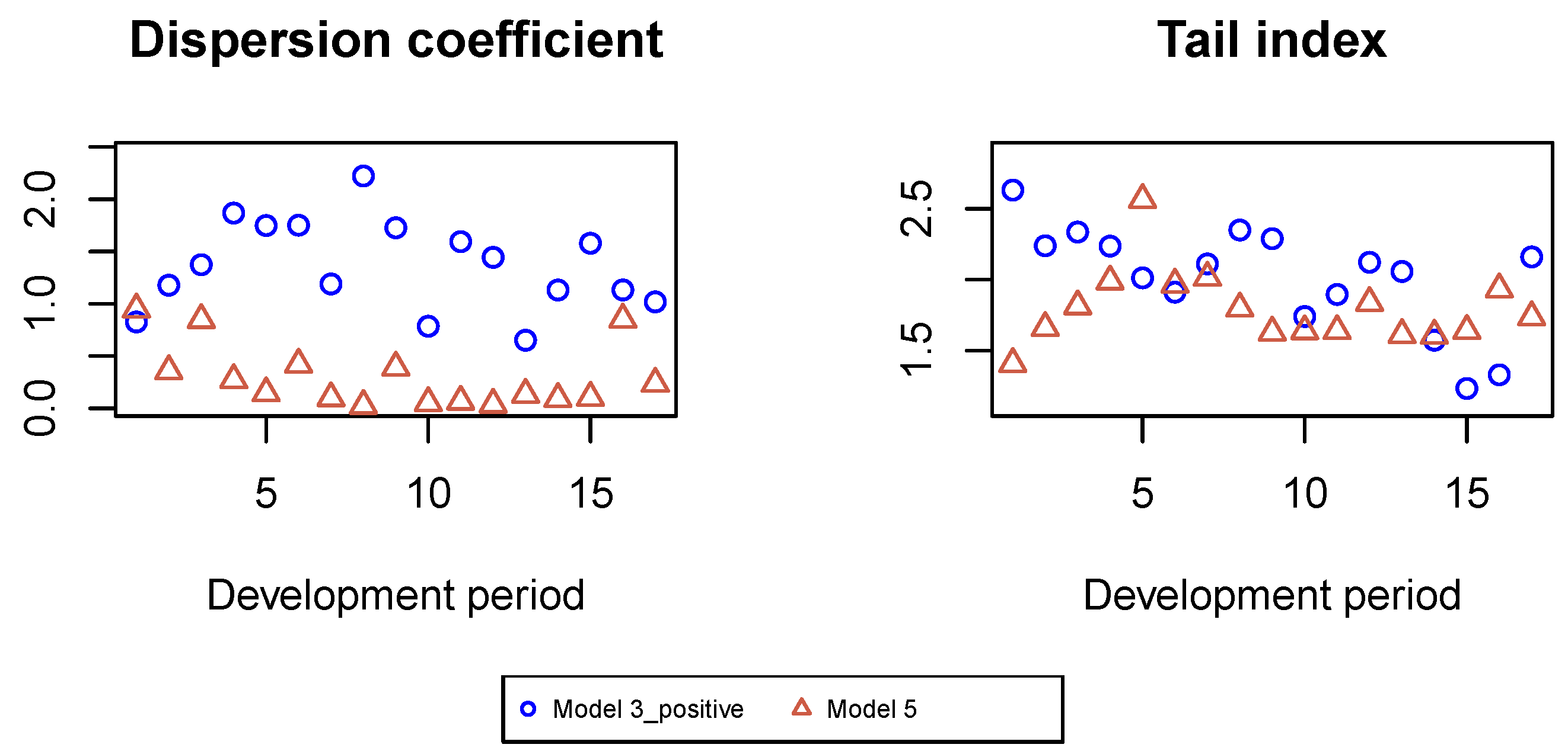
Figure A18 we present the estimated tail indices of Pareto distributions for large claims for all development periods. Moreover, the mean values of the dispersion coefficients estimated for individual claims in Models 3_positive and 5 with the second Gamma regression model, which coincide with the constant dispersion coefficients in the first Gamma regression model, are presented in
Figure A18.
5. Projection to Ultimate Payments for RBNS Claims
In the first step, we use Chain-Ladder techniques to estimate the ultimate payments for RBNS claims. In
Table 6 we present the Chain-Ladder estimates of the development factors calculated on quarterly data for aggregate payments and the numbers of reported claims. We use all observations in the period 2005–2018. We can conclude that we deal with an insurance portfolio with long-tailed development patterns, where late development factors for payments are still bigger than 1.
We calculate the Chain-Ladder predictions for the aggregate ultimate payments and the ultimate number of reported claims per each accident quarter. Next, we calculate the average ultimate payment per accident quarter by diving these two predictions by each other. To differentiate the ultimate payment by the reporting delay of the claim, we calculate the mean values of the claims incurred available at the end of December 2018 per reporting delay and we regress the mean value of the claims incurred versus the reporting delay. We use a GAM regression model to obtain the scaling factors for ultimate payments for claims reported with reporting delays compared to the ultimate payment for a claim reported without a delay. Using the average ultimate payments per accident quarter and reporting delay and the number of claims to be reported in the future periods, we can calculate the IBNYR (Incurred But Not Yet Reported) and RBNS reserves. The aggregate ultimate payments for RBNS claims per accident quarter are calculated as the predicted aggregate ultimate payments for the portfolio minus the predicted number of claims to be reported in the future periods times the average ultimate payment taking into account the reporting delay of the claims (IBNYR). The RBNS reserve is calculated by subtracting the aggregate payments up to December 2018 from the projected aggregate ultimate payments for the RBNS claims. We remark that this is still a rough estimate of the RBNS reserve to receive numbers that are comparable to our individual claim reserving method. The accident years from 2009 till 2018 cover
of the total RBNS reserve of all accident years 2005–2018, so we only focus on these years. The results are presented in
Table 7.
Once Models 1, 3_positive, 4 and 5 are calibrated, we can use them to simulate incremental payments in consecutive development periods (quarters) and generate ultimate payments for RBNS claims. Since we deal with a very large portfolio of claims, we do not have to perform many simulations to receive stable results, unless we are interested in a very high quantile of aggregate ultimate payments. We use 50 simulations, which is sufficient for the results we present below. We consider the claims from the years 2009–2018 but we model their development over the full 55 development periods.
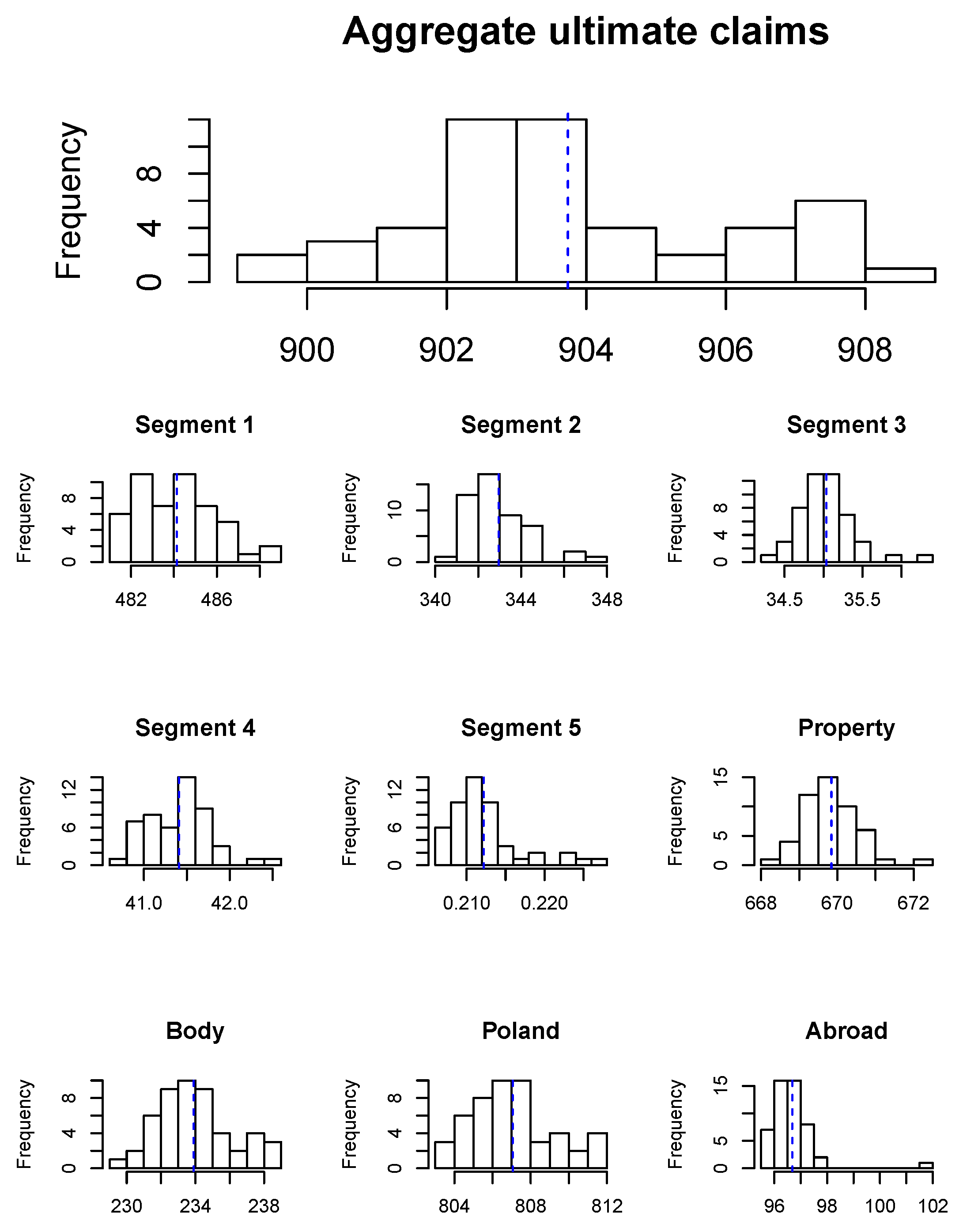
In
Figure 1 we present histograms of the aggregate ultimate payments for the whole insurance portfolio, as well as for segments and different claim features (property versus bodily injury and Poland versus abroad). Such results can help the insurer to improve claims reserving as the insurer can now set claims reserves for policies grouped by claim features. Even at the portfolio level, we expect that the mean prediction from our models should be more precise than the Chain-Ladder estimate derived from aggregate data since our models are calibrated based on detail information about the claim development process, they can cope with seasonality and with changes in portfolio mix. In our case, the proportion of body claims in the portfolio decreases from
in 2005 to
in 2018, and the proportion of the claims caused abroad decreases from
to
. Since body claims and claims from abroad are expected to be the most severe, the Chain-Ladder estimates might be overestimated for the recent accident periods. Apart from calculating the best estimate of liabilities, the histograms in
Figure 1 can also help the insurer to understand which claim features generate the most uncertainty of future payments. Such results can be used to calculate risk adjustments in IFRS 17 or define a safety buffer in claims reserves. We remark that there is a peak in the right tail of the histogram of the aggregate ultimate payments. We conclude that the portfolio is exposed to large claims, which mainly occur in late development periods from body claims and claims from abroad.
In
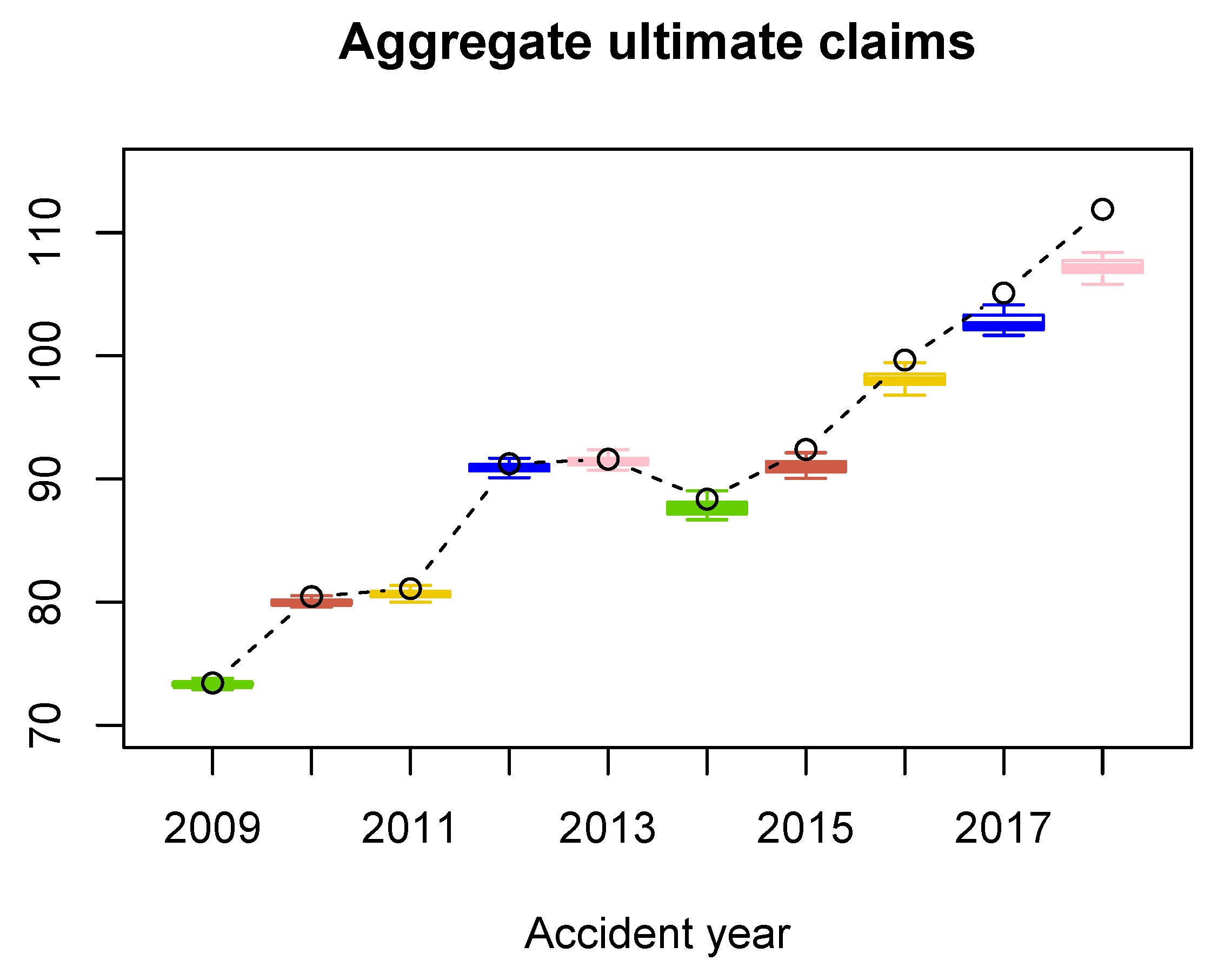
Figure 2 we find boxplots of the aggregated ultimate payments per accident year. Deviations in the simulated payments are small which justifies a small number of simulations, see also 25th and 75th quantiles in
Table 7. In
Figure 2 we compare the ultimate payments for the RBNS claims simulated with our model with the results estimated with the Chain-Ladder technique, and in
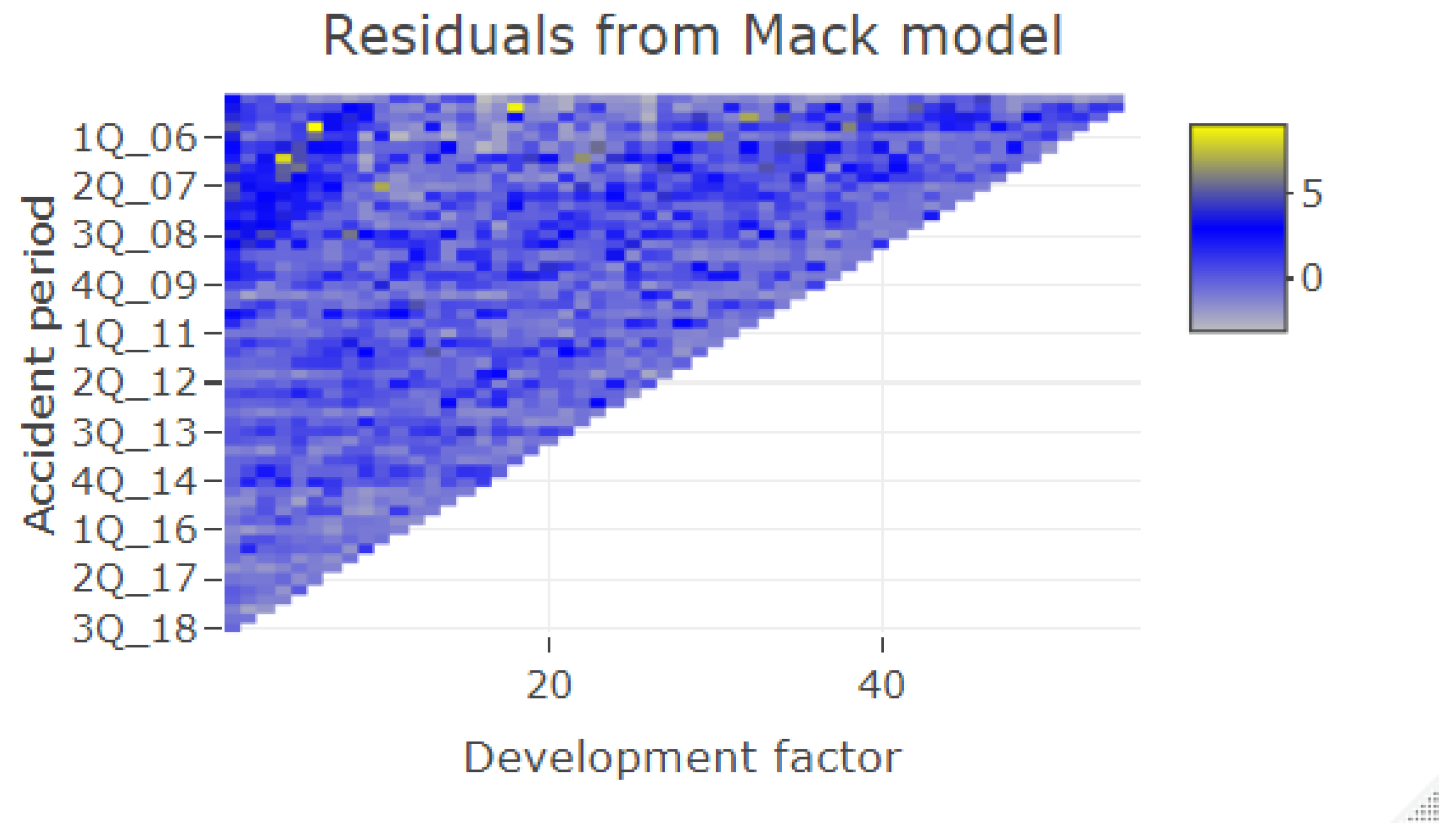
Table 7 we compare the RBNS reserves. We can observe that our model produces lower numbers for the years 2009–2018 than the Chain-Ladder estimates. This observation may be explained with the change of the proportion of body claims and claims from abroad in the insurance portfolio, which we discuss above. Moreover, the Chain-Ladder development factors for old accident years and early development periods tend to be systematically higher than the development factors for recent accident years, see
Figure A19 where dark blue points cumulate in the top left corner of the triangle, especially for the first development period for the old accident years. Consequently, the Chain-Ladder development factors tend to overestimate the future payments.
We can also compare the company’s case reserves with the RBNS reserves estimated with our model, see
Table 7. The comparison is not obvious since case reserves depend on company’s claims reserving policy. For some old accident years the case reserves are above the RBNS reserves. This might be caused by the fact that for old claims, which are not closed, the case reserve is not revaluated and is kept unchanged until the full settlement is made. For recent accident years the case reserves are below the RBNS reserves, as expected.
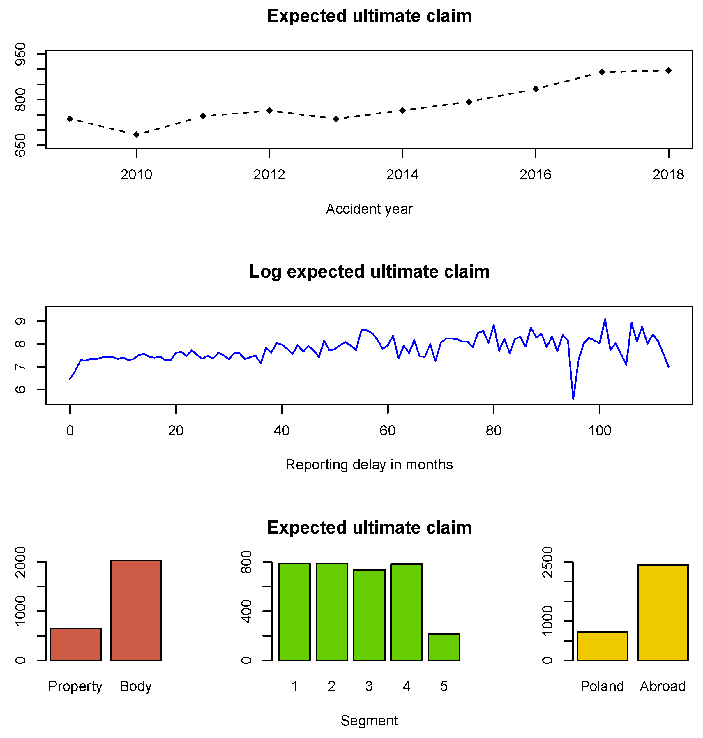
We estimate the expected ultimate payment for an individual claim, see
Figure 3. It agrees with our intuition that the expected ultimate payment for a property claim is lower than for bodily injury one. It also agrees with our intuition that the expected ultimate payment for a claim caused in Poland is lower than for a claim caused abroad. We can also confirm that the expected ultimate payment for an individual claim increases with the reporting delay of the claim.
Finally, we check stability of our calibration procedure. We re-calibrate all neural networks and we re-simulate the developments of all reported claims. When refitting the neural networks, we also change the split of the data of training and validation sets and, this time, we use
of observations as training set and the remaining
as test set. The results are presented in
Table 8. Comparing
Table 7 and
Table 8, we can conclude that the calibration procedure is very stable on the aggregate level (see RBNS reserves of
vs.
). Bigger changes are only observed on older accident years where RBNS are very low and, thus, only marginally contribute to the overall RBNS reserves. This uncertainty on older claims is, of course, caused by the fact that payments for these claims are very rare because most of the claims were already settled.


