Abstract
This note revisits the ideas of the so-called semiparametric methods that we consider to be very useful when applying machine learning in insurance. To this aim, we first recall the main essence of semiparametrics like the mixing of global and local estimation and the combining of explicit modeling with purely data adaptive inference. Then, we discuss stepwise approaches with different ways of integrating machine learning. Furthermore, for the modeling of prior knowledge, we introduce classes of distribution families for financial data. The proposed procedures are illustrated with data on stock returns for five companies of the Spanish value-weighted index IBEX35.
JEL Classification:
C14; C53; C58; G17; G22; C45
1. Introduction
The Editors of this Special Issue pointed out that machine learning (ML) has no unanimous definition. In fact, the term “ML”, coined by Samuel (1959), is quite differently understood in the different communities. The general definition is that ML is concerned with the development of algorithms and techniques that allow computers to learn. The latter means a process of recognizing patterns in the data that are used to construct models; cf. “data mining” (Friedman 1998). These models are typically used for prediction. In this note, we speak about ML for data based prediction and/or estimation. In such a context, one may say that ML refers to algorithms that computer codes apply to perform estimation, prediction, or classification. As said, they rely on pattern recognition (Bishop 2006) for constructing purely data-driven models. The meaning of “model” is quite different here from what “model” or “modeling” means in the classic statistics literature; see Breiman (2001). He speaks of the data modeling culture (classic statistics) versus the algorithmic modeling coming from engineering and computer science. Many statisticians have been trying to reconcile these modeling paradigms; see Hastie et al. (2009). Even though the terminology comes from a different history and background, the outcome of this falls into the class of so-called semi-parametric methods; see Ruppert et al. (2003) or Härdle et al. (2004) for general reviews. According to that logic, ML would be a non-parametric estimation, whereas the explicit parametrization forms the modeling part from classic statistics.
Why should this be of interest? The Editors of this Special Issue also urge practitioners not to ignore what has already been learned about financial data when using presumably fully automatic ML methods. Regarding financial data for example, Buch-Larsen et al. (2005), Bolancé et al. (2012), Scholz et al. (2015, 2016), and Kyriakou et al. (2019) (among others) have shown the significant gains in estimation and prediction when including prior knowledge in nonparametric prediction. The first two showed how knowledge-driven data transformation improves nonparametric estimation of distribution and operational risk; the third paper used parametrically-guided ML for stock return prediction; the fourth imputed bond returns to improve stock return predictions; and the last proposed comparing different theory-driven benchmark models regarding their predictability. Grammig et al. (2020) combined the opposing modeling philosophies to predict stock risk premia. In this spirit, we will discuss the combination of purely data-driven methods with smart modeling, i.e., using prior knowledge. This will be exemplified along the analysis of the distributions (conditional and unconditional) of daily stock returns and calculations of their value-at-risk (VaR).
Notice finally that in the case of estimation, methods are desirable that permit practitioners to understand, maybe not perfectly, but quite well, what the method is doing to the data. This will facilitate the interpretation of results and any further inference. Admittedly, this is not always necessary and certainly also depends on the knowledge or imagination of the user. Yet, we believe it is often preferable to analyze data in a glass box than in a black box. This aspect is respected in our considerations.
2. Preliminary Considerations and General Ideas
It is helpful to first distinguish between global and local estimation. Global means that the parameter or function applies at any point and to the whole sample. Local estimation applies only to a given neighborhood, like for kernel regression. It is clear that localizing renders a method much more flexible; however, the global part allows for an easy modeling, and its estimation can draw on the entire sample. Non-parametric estimators are not local by nature; for example, power series based estimators are not. Unless you want to estimate a function with discontinuities, local estimators are usually smoothing methods; see Härdle et al. (2004). This distinction holds also for complex methods (cf. the discussion about extensions of neural networks to those that recognize local features), which often turn out to be related to weighted nearest neighbor methods; see Lin and Jeon (2006) for random forests or Silverman (1984) for splines. The latter is already a situation where we face a mixture of global and local smoothing; another one is orthogonal wavelet series (Härdle et al. 1998).
Those mixtures are interesting because the global parts can borrow the strength from a larger sample and have a smoothing effect, while the local parts allow for the desired flexibility to detect local features. Power series can offer this only by including a (in practice unacceptable) huge number of parameters. This is actually a major problem of many complex methods, but mixtures allow substantially reducing this number. At the same time, they allow us to include prior knowledge about general features. For example, imposing shape restrictions is much simpler for mixtures (like splines) than it is for purely local smoothers; see Meyer (2008) and the references therein. Unless the number of parameters is pre-fixed, their selection happens via reduction through regularization, which can be implemented in many ways. Penalization methods like P-splines (Eilers et al. 2015) or LASSO (Tibshirani 1996) are popular. The corresponding problem for kernel, nearest neighbors, and related methods is the choice of the neighborhood size. In any case, one has to decide about the penalization criterion and a tuning parameter. The latter is until today an open question; presently, cross-validation-type methods are the most popular ones. For kernel based methods, see Heidenreich et al. (2013) and Köhler et al. (2014) for a review or Nielsen and Sperlich (2003) in the context of forecasting in finance.
The first question concerns the kind of prior information available, e.g., whether it is about the set of covariates, how they enter (linearly, additively, with interactions), the shape (skewness, monotonicity, number of modes, fat tails), or more generally, about smoothness. This is immediately followed by the question of how this can be included; in some cases, this is obvious (like if knowing the set of variables to be included); in some others, it is more involved (like including parameter information via Bayesian modeling). Knowledge about smoothness is typically supposed in order to justify a particular estimator and/or the selection method for the smoothing parameter. Information about the shape or how covariates enter the model comprises the typical ingredients of semiparametric modeling (Horowitz 1998) to improve nonparametric estimation (Glad 1998).
Consider the problem of estimating a distribution, starting with the unconditional case. In many situations, you are more interested in those regions for which data are hardly available. If you used then a standard local density estimator, you would try to estimate interesting parameters like VaR from only very few observations, maybe one to five, which is obviously not a good idea. Buch-Larsen et al. (2005) proposed to apply a parametric transformation using prior knowledge. Combining this way a local (kernel density) estimator with such a global one, however, allowed them to borrow strength from the model and from data that were further away. Similarly, consider conditional distributions. Locally, around a given value of the conditioning variable, you may have too few observations to estimate a distribution nonparametrically. Then, you may impose on this neighborhood the same probability law up to some moments, as we will do in our example below.1
Certainly, a good mixture of global and local fitting is problem-adapted. Then, the question falls into two parts: which is the appropriate parametric modeling, and how to integrate it with the flexible local estimator. For the former, you have to resort to expertise in the particular field. For the latter, we will discuss some popular approaches. All this will be exemplified with the challenges of modeling stock returns for five big Spanish companies and predicting their VaR.
In our example, the first step is to construct a parametric guide for the distribution of stock returns Y. To this aim, we introduce the class of generalized beta-generated (BG) distributions (going back, among others, to Eugene et al. (2002) and Jones (2004)), as this distribution class allows modeling skewed distributions with potentially long or fat tails. While this is not a completely new approach, we present it with an explicit focus on the above outlined objectives including the calculation of VaRs and combining it with nonparametric estimation and/or validation. Our validation is more related to model selection and testing, today well understood and established, and therefore kept short. The former, i.e., the combination with nonparametric estimation, is discussed for the problem of analyzing conditional distributions and can be extended to the combination with methods for estimating in high dimensions. For this example, in which the prior knowledge enters via a distribution class, we discuss two approaches: one is based on the method of moments, the other one on maximum likelihood. The latter is popular due to Rigby and Stasinopoulos (2005) and Severini and Staniswalis (1994). Rigby and Stasinopoulos (2005) considered a fully parametrized model in which each distribution parameter (potentially transformed with a known link) is written as an additive function of covariates, typically including a series of random effects. They proposed a backfitting algorithm (implemented in the R library GAMLSS) to maximize a penalized likelihood corresponding to a posterior mode estimation using empirical Bayesian arguments. Severini and Staniswalis (1994) started out with the parametric likelihood, but localized it by kernels. This is maximized then for some given values of the covariates.
3. A Practical Example
We now discuss the technical steps for the announced practical example. While this section focuses on the technical part, the empirical exercise is done in the next section.
3.1. Distribution Modeling
Often, the Student t distribution was used in financial econometrics and risk management to model the conditional asset returns, going back to Bollerslev (1987). However, it is well known that it does not describe very well the empirical features of most financial data. Therefore, several proposals have been made of skewed Student t distributions; see Theodossiou (1998) and Zhu and Galbraith (2010) for the context of finance or Jones and Faddy (2003) and Azzalini and Capitanio (2003) in (applied) statistics. For a more general discussion and compendium, see Rigby et al. (2019).
Let us consider two classes of skewed t distributions. Both are derived from the (generalized) BG classes; see Appendix A. These allow for the generation of many flexible distribution classes. The fist version depends on two parameters, whereas the second one depends on three. One may directly go for the second one. Remember, however, later on, that this is just a parametric guide for the semiparametric estimator. There is certainly a trade-off between the gain of flexibility, on the one hand, and the loss of its regularization, on the other hand. Moreover, each additional parameter in the global part may raise the costs of implementation and computation to an unacceptable degree. Both skewed t distributions are generated by taking a standard Student t as the baseline distribution in (A1) and (A2), respectively. Specifically, plugging in , a so-called scaled Student , into (A1), gives our skewed t of Type 1 with the probability density function (pdf):
where and . We write ; see Jones and Faddy (2003). Plugging the baseline cumulative density (cdf) into (A2) gives our skewed t of Type 2 with the pdf:
where and . We write ; see Alexander and Sarabia (2010) and Alexander et al. (2012). The densities , are illustrated in Figure 1.
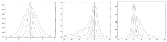
For implementation, estimation, model selection, and in particular, for the possible integration of ML, we take a closer look at the basic properties of these two distributions. Note that for in (1), one obtains the classical Student t distribution with degrees of freedom. The same is true for the three-parameter case (2) when setting with . Furthermore, the cdfs are given by:
and:
respectively. Having explicit expressions for the pdf, one may think that likelihood based methods are straight-forward, including those for tests and model selection. Note, however, that for a sample of size m, you need to know the joint distribution of , which are not independent. In practice, many work with , ( with for , else) as a likelihood approximate, ignoring potential dependencies. This weakens both the efficiency of estimation and the validity of likelihood based inference. Therefore, it is interesting to look at alternatives. For estimation, recall the moment based approach; then, we need to to express parameters , and if applicable c, in terms of estimable moments. For the case of the skewed t distribution of the first kind, we have:
if . An advantage of this expression is that we do not need to estimate the centered, standardized moments. This is even more an advantage when we try to estimate these moments nonparametrically. Similarly, for the skewed t distribution of the second kind:
Clearly, this reveals a problem because we cannot solve this (easily) for , and c.
3.2. Financial Risk Measures
The parametric part provides us with explicit formulas that we can use to derive closed expressions for the risk measures, namely the VaR and tail moments. In fact, it can be shown that:
with , where denotes the VaR of a classical distribution. Furthermore, if , then the for a given , its corresponding tail moments can we written as:
where and which is increasing in z, with . For , we get the T(ail)VaR. If , then one has:
where , , and as above. In sum, for the Type 1 class, we obtain explicit expressions for the tail moments that do not change when are functions of covariates.
3.3. Combining The Prior with Nonparametric Estimation
First, let us briefly consider the case of being only interested in the estimation of the unconditional distribution , say, in that of stock returns Y. Once a proper parametric choice (say ) is found and the parameters are estimated, we know that has a pretty smooth density , which is not too far from the uniform distribution. Then, as , you obtain the final estimate. A next step to proceed could be to apply a nonparametric estimator like, for example, a kernel density for . The prior estimation served here to stretch data where we had many observations, and contract them where we had only a few. You may say that this could also be done either by taking the empirical cdf for transformation or by taking the local bandwidth that always includes the same number of neighbors. This would be purely nonparametric and therefore renounce the use of prior information. In practice, these alternatives suffer from various problems like giving wiggly results, a much harder bandwidth choice, etc. For details and applications in actuarial sciences, consult Bolancé et al. (2012) and Martínez Miranda et al. (2009).
We turn now to the slightly more challenging problem of considering conditional distributions. For example, what is the stock return distribution of Telefónica and its VaR given a certain value of the Spanish IBEX35? Having huge datasets, you may try to estimate this with a fully nonparametric estimator. However, if you doubt that stationarity holds over a long period, you may want to restrict your dataset to not include more than twelve months (as an example). In such a case, you better resort to a parametric guide like above and turn (and c if applicable) into flexible functions of the conditioning covariate X. Again, a likelihood based approach may now look at ( with for , etc.) ignoring potential dependencies. Rigby and Stasinopoulos (2005) specified the elements of as additive, parametrized functions of with some random coefficients, and maximized a penalized version of this. In contrast, Severini and Staniswalis (1994) did not parametrize the elements of , but maximized (along ) the smoothed version, i.e., for any x. Here, for a kernel function with bandwidth h. That is, they obtained for given x an estimate of the value that takes at x. Notice that the latter method is usually implemented for containing only one element (typically the mean).
As said before, an interesting alternative is to estimate nonparametrically the moments of Y and then derive the elements of . Thanks to Formula (5), we can do this for the Type 1 skewed t distributions. More specifically, the algorithm would look as follows: For sample , with being the return of the stock and the conditioning variable (in our application, the market return) conduct:
Step 1: Estimate the conditional first two moments and by:
where the nonparametric functions can be estimated, e.g., by kernel regression, splines, etc.
Step 2: You now may either take a grid over the range of X, with M grid points , or you may calculate the estimates for each observation . Let us call them and , for either case.
Step 3: Calculate estimates by solving in , , the non-linear system:
Step 4: Then, the estimate of the conditional distribution is of the form:
Following Nielsen and Sperlich (2003), Kyriakou et al. (2019), and Mammen et al. (2019), you could use local linear regression in Step 1 for both functions, combined with the validated for the bandwidth choice. Obviously, any method known as ML, including LASSO variable selection, can be applied in this step. However, it is less evident how these methods could be combined with the aforementioned likelihood based approaches. Note further that the conditional distribution obtained by this strategy can also be used for semiparametric prediction of the unconditional distribution:
This shows that with , , you can predict the marginal distribution of Y for scenarios in which the distribution of X is changing (Dai et al. 2016). For example, we could predict the unconditional distribution of stocks for different distributions of the IBEX35. Note finally that Step 3 cannot easily be applied to the skewed t distribution of Type 2; recall (6). In such a case, you could only try to apply the idea of Rigby and Stasinopoulos (2005), but with procedures and algorithms that are still to be developed.
4. Empirical Illustration
Consider daily stock returns from 1 January 2015 to 31.12.2015 for five companies of the Spanish value-weighted index IBEX35; namely Amadeus (IT solutions for tourist industry), BBVA (global financial services), Mapfre (insurance market), Repsol (energy sector), and Telefónica (information and communications technology services); see Table 1. The returns are negatively skewed in four of the five companies considered, but positively skewed in the last one.

Table 1.
Summary statistics. The sample size is for all sets.
We first fit the data by the maximum likelihood (ignoring dependence) to both distribution classes, working with standardized data. Table 2 and Table 3 show the parameter estimates with standard errors.
Table 2.
Maximum likelihood estimates for the skewed t model of Type 1, standardized data. Standard errors are in parenthesis.
Table 3.
Maximum likelihood estimates for the skewed t model of Type 2, standardized data. Standard errors are in parenthesis.
To choose between these two models, one may use the Bayesian information criterion (BIC). However, as our (working) likelihood neglects the dependence structure, it might not be reliable. While the three-parameter model presents the largest values for BIC (not shown), the gain, however, is always close to, or smaller than, 1%.
An alternative is to apply ML methods comparing the parametric estimates with purely nonparametric ones. This is not recommendable any longer when switching to conditional distributions due to the moderate sample sizes. In Figure 2, you see how our models (in red) adapted to the empirical cdf (blue) for the stocks of Amadeus and BBVA. As expected, the three-parameter model gave slightly better fits. In practice, the interesting thing to see is where improvements occurred, if any. The practitioner has to judge then what is of interest for his/her problem; ML cannot do this for him/her. However, ML can offer specification tests; see Gonzales-Manteiga and Crujeiras (2013) for a review. For example, a test that formalizes our graphical analysis is the Kolmogorov–Smirnov () test:
where is the empirical cdf and is the cdf of the particular model class with from Table 2 and Table 3. To calculate the p-value, we can use the parametric bootstrap:
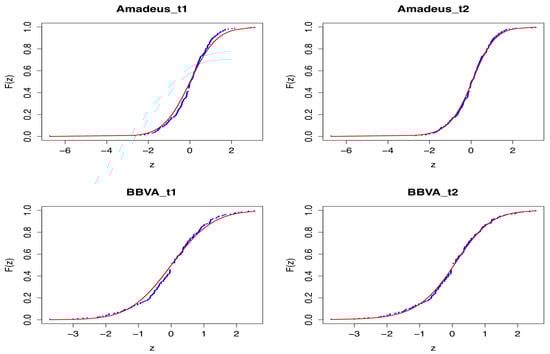
Figure 2.
Plots of the theoretical cdfs of the skewed t models (LEFT: model; RIGHT: model) and the empirical cdf. Stocks: Amadeus; BBVA.
Step 1: For the observed sample, find the maximum likelihood estimator, , , and .
Step 2: Generate J bootstrap samples under (the data follow model F); fit them; and compute , , and for each bootstrap sample .
Step 3: Calculate the p-value as the fraction of synthetic bootstrap samples with a statistic greater than the empirical statistic obtained from the original data.
To obtain an approximate accuracy of the p-value for 0.01, we generated bootstrap samples. Table 4 shows the results for both distribution classes and all datasets. It can be seen that with all p-values larger than 0.499, both models could not be rejected at any reasonable significance level in any of the considered datasets.
Table 4.
Bootstrap p-values for both models and all five datasets.
Finally, let us see how different the VaR are, when calculated on the base of one model compared to the other; recall Equations (7) and (8). They were calculated at the 95% confidence level for all datasets; see Table 5. The model with two parameters provided slightly higher VaR values than the model. The difference again seemed to be somewhat marginal, except maybe for Amadeus.
Table 5.
Values at risk and for the five stocks considered.
Let us turn to the estimation of the conditional distribution. Here, the integration of the ML happens by incorporating the covariates nonparametrically. For the sake of presentation and brevity, we restricted ourselves here to the moment based approach; for more details on the likelihood based one, we refer (besides the above cited literature) to the recent compendium of Rigby et al. (2019) and the references therein. Limiting ourselves to the moment based method automatically limited us to the skewed t1 class; recall Equation (6).2 Furthermore, for the sake of illustration, we limited the exercise to the estimation of all distribution parameters as nonparametric functions of one given covariate X, namely the IBEX35. It was obvious that estimates for , could equally well be the result of a complex multivariate regression or a variable selection procedure like LASSO. We estimated (IBEX35) and (IBEX35) using different methods provided by standard software; the presented results were obtained from penalized (cubic) spline regression with data-driven penalization. For details, consult Ruppert et al. (2003) and the SemiPar project. Figure 3 gives an example of how this performed for the BBVA stocks.
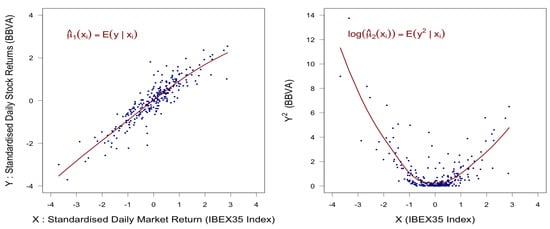
Figure 3.
Estimates , for BBVA stock returns as functions of IBEX35.
Table 6 gives for the IBEX35 quantiles , , the corresponding moment estimates of the different stock returns; Table 7 the corresponding for Formulas (10) and (11). Table 8 gives the corresponding conditional VaRs obtained from Formula (7).
Table 6.
First two moments of stock returns for given IBEX35 values (looking at its quantiles).
Table 7.
Parameter of the conditional stock return distributions for given IBEX35 values.
Table 8.
The conditional value at risk for given IBEX35 values.
In Figure 4, you can see the entire conditional distributions for the three IBEX35 quantiles. Finally, in Figure 5, we plotted the resulting unconditional distributions when you integrate over the observed IBEX35 values; recall Equation (12). They reflect quite nicely the asymmetries and some fat tails.
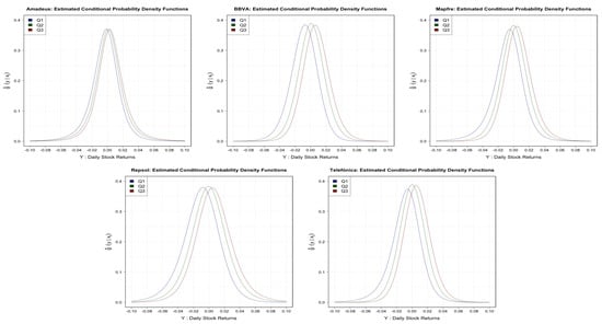
Figure 4.
Conditional densities of stock returns at the quantiles of IBEX35 for Amadeus (upper left), BBVA (upper center), Mapfre (upper right), Repsol (lower left), and Telefónica (lower right).
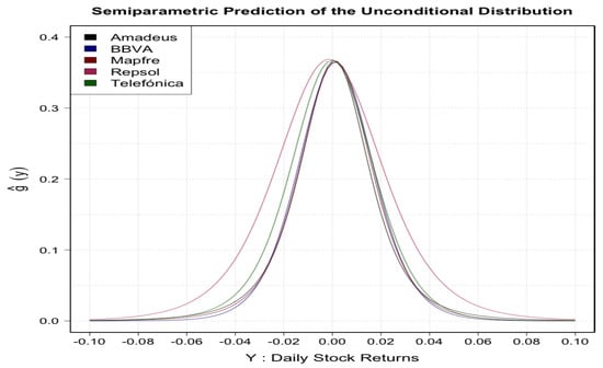
Figure 5.
Unconditional densities of stock returns obtained from integrating the conditional ones over all observed IBEX35 values.
5. Discussion and Conclusions
In this note, we revisited the ideas of semiparametric modeling to propose for ML what one could call glass box modeling. It integrates ML in a mixture of a global and a local part in which the global one is as a parametric guide for the nonparametric estimate. We discussed different advantages of such a kind of smart modeling and the steps to be performed. In our illustration (analyzing financial data), we proposed as a parametric guide some (generalized) beta-generated distributions. In particular, we considered two classes of skewed t distributions. This allowed us to work with analytical expressions for the pdf, cdf, moments, and quantile functions, including the VaR, even on a local level. An empirical application with five datasets of stock returns was performed for illustration.
Author Contributions
All authors (J.M.S., F.P., V.J., S.P.) contributed equally to this work. All authors have read and agreed to the published version of the manuscript.
Funding
The authors thank the Institute and Faculty of Actuaries in the U.K. for funding their research through the grant “Minimizing Longevity and Investment Risk while Optimizing Future Pension Plans” and the Spanish Ministerio de Economía y Competitividad, Project ECO2016-76203-C2-1-P, for partial support of this work.
Conflicts of Interest
The authors declare no conflict of interest.
Appendix A. Some Classes of Beta-Generated Distributions
This is to recall the class of BG distributions and to present some basic properties of this class. Let us call pdf the baseline probability function with being the corresponding cdf. The class of BG distributions is defined in terms of the pdf by:
where denotes the gamma function and some real numbers. If for m being the sample size, we set and in (A1), one obtains the pdf of the ith order statistic from F (Jones 2004). For , we obtain a family of skewed distributions, for and the distribution of the maximum, for and the one of the minimum, and for obviously . In our context, the first property is the most interesting one. The parameters a and b control the tailweight of the distribution, where a controls the left-hand and b the right-hand tailweight. Consequently, for , one obtains a symmetric sub-family, but still with controlling the tailweight. The BG distribution accommodates several kinds of tails like potential and exponential ones (Jones 2004).
For the moment method and in order to express the VaR in terms of moments or , we need to relate to (directly) estimable moments. Let us now denote the cdf associated with (A1) by with denoting the incomplete beta-function ratio:
where , such that . For a random variable , i.e., following the classical beta distribution, a simple stochastic representation of (A1) is This allows for a direct simulation of the values of a random variable with pdf (A1). The raw (i.e., not centered, not normalized) moments of a BG distribution can be obtained by:
Recently, some extensions have been proposed, e.g., by Alexander and Sarabia (2010), Alexander et al. (2012) and Cordeiro and de Castro (2011), of which we consider the one towards three parameters: The generalized BG (GBG) distribution is defined for by the pdf:
For , we get the BG distribution; for , one obtains the so-called proportional hazard model; and setting yields the so-called Kumaraswamy generated distribution.
References
- Alexander, Carol, and José-María Sarabia. 2010. Generalized Beta-Generated Distributions. In ICMA Centre Discussion Papers in Finance DP2010-09. Reading: ICMA Centre. [Google Scholar]
- Alexander, Carol, Gauss M. Cordeiro, Edwin M. M. Ortega, and José-María Sarabia. 2012. Generalized beta-generated distributions. Computational Statistics & Data Analysis 56: 1880–97. [Google Scholar]
- Azzalini, Adelchi, and Antonella Capitanio. 2003. Distributions generated by perturbation of symmetry with emphasis on a multivariate skew t-distribution. Journal of the Royal Statistical Society. Series B 65: 367–89. [Google Scholar] [CrossRef]
- Bishop, Christopher M. 2006. Pattern Recognition and Machine Learning. Heidelberg: Springer. [Google Scholar]
- Bolancé, Catalina, Montserrat Guillén, Jim Gustafsson, and Jens Perch Nielsen. 2012. Quantitative operational Risk Models. New York: Chapman & Hall/CRC Finance. [Google Scholar]
- Bollerslev, Tim. 1987. A Conditionally Heteroskedastic Time Series Model for Speculative Prices and Rates of Return. The Review of Economics and Statistics 69: 542–47. [Google Scholar] [CrossRef]
- Breiman, Leo. 2001. Statistical Modeling: The Two Cultures. Statistical Science 16: 199–231. [Google Scholar] [CrossRef]
- Buch-Larsen, Tine, Jens Perch Nielsen, Montserrat Guillén, and Catalina Bolancé. 2005. Kernel density estimation for heavy-tailed distributions using the Champernowne transformation. Statistics 39: 503–18. [Google Scholar] [CrossRef]
- Cordeiro, Gauss M., and Mário de Castro. 2011. A new family of generalized distributions. Journal of Statistical Computation and Simulation 81: 883–93. [Google Scholar] [CrossRef]
- Dai, Jing, Sefan Sperlich, and Walter Zucchini. 2016. A simple method for predicting distributions by means of covariates with examples from welfare and health economics. Swiss Journal of Economics and Statistics 152: 49–80. [Google Scholar] [CrossRef]
- Eilers, Paul H. C., Brian D. Marx, and Maria Durbán. 2015. Twenty years of P-splines. Statistics and Operation Research Transactions 39: 149–86. [Google Scholar]
- Eugene, Nicholas, Carl Lee, and Felix Famoye. 2002. The beta-normal distribution and its applications. Communications in Statistics: Theory Methods 31: 497–512. [Google Scholar] [CrossRef]
- Friedman, Jerome H. 1998. Data Mining and Statistics: What’s the connection? Computing Science and Statistics 29: 3–9. [Google Scholar]
- Glad, Ingrid K. 1998. Parametrically guided non-parametric regression. Scandinavian Journal of Statistics 25: 649–68. [Google Scholar] [CrossRef]
- Gonzales-Manteiga, Wenceslao, and Rosa M. Crujeiras. 2013. An updated review of goodness-of-fit tests for regression models. Test 22: 361–411. [Google Scholar] [CrossRef] [PubMed]
- Grammig, Joachim, Constantin Hanenberg, Christian Schalg, and Jantje Sönksen. 2020. Diverging Roads: Theory-Based vs. Machine Learning-Implied Stockrisk Premia. Tübingen, Germany: University of Tübingen Working Papers in Business and Economics, No 130, University of Tübingen. [Google Scholar]
- Härdle, Wolfgang, Gérard Kerkyacharian, Dominique Picard, and Alexander Tsybakov. 1998. Wavelets, Approximation, and Statistical Applications. Heidelberg: Springer. [Google Scholar]
- Härdle, Wolfgang, Marlene Müller, Stefan Sperlich, and Alexander Werwatz. 2004. Nonparametric and Semiparametric Models. Heidelberg: Springer. [Google Scholar]
- Hastie, Trevor, Robert Tibshirani, and Jerome Friedman. 2009. The Elements of Statistical Learning: Data Mining, Inference and Prediction. Heidelberg: Springer. [Google Scholar]
- Heidenreich, Niels-Bastian, Anja Schindler, and Stefan Sperlich. 2013. Bandwidth Selection Methods for Kernel Density Estimation: A review of fully automatic selectors. AStA Advances in Statistical Analysis 97: 403–33. [Google Scholar] [CrossRef]
- Horowitz, Joel L. 1998. Semiparametric Methods in Econometrics. Heidelberg: Springer. [Google Scholar]
- Jones, M. Chris, and M.J. Faddy. 2003. A Skew Extension of the t-Distribution, with Applications. Journal of the Royal Statistical Society. Series B 65: 159–74. [Google Scholar] [CrossRef]
- Jones, M. Chris. 2004. Families of distributions arising from distributions of order statistics. Test 13: 1–43. [Google Scholar]
- Köhler, Max, Anja Schindler, and Stefan Sperlich. 2014. A Review and Comparison of Bandwidth Selection Methods for Kernel Regression. International Statistical Review 82: 243–74. [Google Scholar] [CrossRef]
- Kyriakou, Ioannis, Parastoo Mousavi, Jens Perch Nielsen, and Michael Scholz. 2019. Forecasting benchmarks of long-term stock returns via machine learning. Annals of Operations Research. [Google Scholar] [CrossRef]
- Lin, Yi, and Yongho Jeon. 2006. Random Forests and Adaptive Nearest Neighbors. Journal of the American Statistical Association 101: 578–90. [Google Scholar] [CrossRef]
- Mammen, Enno, Jens Perch Nielsen, Michael Scholz, and Stefan Sperlich. 2019. Conditional Variance Forecasts for Long-Term Stock Returns. Risks 7: 113. [Google Scholar] [CrossRef]
- Martínez Miranda, M. Dolores, Jens Perch Nielsen, and Stefan Sperlich. 2009. One Sided Cross Validation for Density Estimation. In Operational Risk Towards Basel III: Best Practices and Issues in Modeling, Management and Regulation. Edited by Greg N. Gregoriou. Hoboken: John Wiley and Sons, pp. 177–96. [Google Scholar]
- Meyer, Mary C. 2008. Inference using shape-restricted Regression Splines. Annals of Applied Statistics 2: 1013–33. [Google Scholar] [CrossRef]
- Nielsen, Jens Perch, and Stefan Sperlich. 2003. Prediction of stock returns: A new way to look at it. ASTIN Bulletin 33: 399–417. [Google Scholar] [CrossRef][Green Version]
- Rigby, Robert A., and D. Mikis Stasinopoulos. 2006. Generalized additive models for location, scale and shape. Journal of the Royal Statistical Society. Series C 54: 507–54. [Google Scholar] [CrossRef]
- Rigby, Robert A., Mikis D. Stasinopoulos, Gillian Z. Heller, and Fernanda De Bastiani. 2019. Distributions for Modeling Location, Scale, and Shape: Using GAMLSS in R. New York: Chapman & Hall/CRC Finance. [Google Scholar]
- Ruppert, David, Matt P. Wand, and Raymond J. Carroll. 2003. Semiparametric Regression. Cambridge: Cambridge University Press. [Google Scholar]
- Samuel, Arthur. 2006. Some Studies in Machine Learning Using the Game of Checkers. IBM Journal of Research and Development 3: 210–29. [Google Scholar] [CrossRef]
- Scholz, Michael, Jens Perch Nielsen, and Stefan Sperlich. 2015. Nonparametric prediction of stock returns based on yearly data: The long-term view. Insurance: Mathematics and Economics 65: 143–55. [Google Scholar] [CrossRef]
- Scholz, Michael, Stefan Sperlich, and Jens Perch Nielsen. 2016. Nonparametric long term prediction of stock returns with generated bond yields. Insurance: Mathematics and Economics 69: 82–96. [Google Scholar] [CrossRef]
- Severini, Thomas A., and Joan G. Staniswalis. 1994. Quasi-likelihood estimation in semiparametric models. Journal of the American Statistical Association 89: 501–11. [Google Scholar] [CrossRef]
- Silverman, Bernard W. 1984. Spline Smoothing: The Equivalent Variable Kernel Method. Annals of Statistics 12: 898–916. [Google Scholar] [CrossRef]
- Theodossiou, Panayiotis. 1998. Financial Data and the Skewed Generalized T Distribution. Management Science 44: 1650–61. [Google Scholar] [CrossRef]
- Tibshirani, Robert. 1996. Regression Shrinkage and Selection via the lasso. Journal of the Royal Statistical Society. Series B 58: 267–88. [Google Scholar] [CrossRef]
- Zhu, Dongming, and John Galbraith. 2010. A generalized asymmetric Student-t distribution with application to financial econometrics. Journal of Econometrics 157: 297–305. [Google Scholar] [CrossRef]
| 1. | Further advantages are that semiparametric modeling can help to overcome the curse of dimensionality and that semiparametric models are more robust to the choice of smoothing parameters. |
| 2. | You may develop numerical approximations working with (6), but this is clearly beyond the scope of this note. However, the above studies insinuate that the gain by using the more complex Type 2 class is rather marginal. Those advantages get easily compensated by the local estimator. |
© 2020 by the authors. Licensee MDPI, Basel, Switzerland. This article is an open access article distributed under the terms and conditions of the Creative Commons Attribution (CC BY) license (http://creativecommons.org/licenses/by/4.0/).