Article

Quantitative and Comparative Analyses of Limit Order Books with General Compound Hawkes Processes

Department of Mathematics and Statistics, University of Calgary, 2500 University Drive NW, Calgary, AB T2N1N4, Canada
*
Author to whom correspondence should be addressed.
Risks 2019, 7(4), 110; https://doi.org/10.3390/risks7040110
Submission received: 30 June 2019 / Revised: 17 September 2019 / Accepted: 25 October 2019 / Published: 1 November 2019

Abstract

:
In this paper, we solve the problem of mid price movements arising in high-frequency and algorithmic trading using real data. Namely, we introduce different new types of General Compound Hawkes Processes (GCHPDO, GCHP2SDO, GCHPnSDO) and find their diffusive limits to model the mid price movements of 6 stocks-EBAY, FB, MU, PCAR, SMH, CSCO. We also define error rates to estimate the models fitting accuracy. Maximum Likelihood Estimation (MLE) and Particle Swarm Optimization (PSO) are used for Hawkes processes and models parameters’ calibration.

1. Introduction

Big data has now become a driver of model building and analysis in a number of areas, including finance. More than half of the markets in today’s highly competitive and relentlessly fast-paced financial world now use a limit order book (LOB) mechanism to facilitate trade. The main problem here is how to deal with big data arising in electronic markets for algorithmic and high-frequency (milliseconds) trading (HFT).
The present paper introduces new different types of general compound Hawkes processes (GCHP)—namely GCHPDO (two fixed ticks, + δ , δ , dependent orders), GCHP2SDO (two non-fixed ticks, ( a ( 1 ) , a ( 2 ) ) , dependent orders) and GCHPnSDO (n non-fixed ticks, ( a ( 1 ) , , a ( n ) ) , dependent order)—to model the mid prices S t dynamics of the assets in HFT, namely, EBAY, FB, MU, PCAR, SMH, CSCO, (provided by Reference Cartea et al. (2015)).
As we mentioned, high-frequency trading happens in milliseconds, as order arrivals and cancellations are very frequent. How we can study and model the dynamics of the mid-prices? One of the ways is to look over a larger time scale, for example, 5, 10 or 20 min, that is, consider time scale n t instead of t , then n could be n = 100 , 1000 , , etc. It means that we consider the dynamics of order flow over large time scales. Thousands of order book events may occur over such large time scales (e.g., for CISCO data on one day in 2014 it is around 500,000, see Reference Cartea et al. (2015)). Thus, we can use asymptotic methods to study the link between order flow and price volatility by considering the diffusive limit of the mid-price processes. More precisely, we use the functional central limit theorems for above-mentioned GCHP and present the volatility of price changes in terms of the parameters of initial models.
To estimate the models fitting accuracy we define an error rate for each model and set the threshold value as 15 % . The model with error rate less than the threshold is considered as well fitted. Thus, we define which of our models is the best fit for our real data.
We also use Maximum Likelihood Estimation (MLE) and Particle Swarm Optimization (PSO) for Hawkes processes and our parameters’ calibration.
There are many papers devoted to the modelling of HFT and applications of Hawkes processes in finance. See Reference Bacry et al. (2015) for more details. Below we give an overview of the most relevant literature.
Reference Cont and De Larrard (2013) proposed a simple Markovian stochastic model for the dynamics of a limit order book, in which arrivals of market orders, limit orders and order cancellations are independent and inter-arrival times have exponential distribution. They also studied the diffusion limit of the price process and expressed the volatility of price changes in terms of parameters describing the arrival rates of buy and sell orders and cancellations.
As suggested by empirical observations, Reference Swishchuk and Vadori (2017) extended their framework to (1) arbitrary distributions for book events inter-arrival times (possibly non-exponential) and (2) both the nature of a new book event and its corresponding inter-arrival time depend on the nature of the previous book event. They did so by resorting to Markov renewal processes to model the dynamics of the bid and ask queues. They kept analytical tractability via explicit expressions for the Laplace transforms of various quantities of interest. They also justified and illustrated their approach by calibrating their model to the five stocks Amazon, Apple, Google, Intel, Microsoft on 21 June 2012, to the 15 stocks from Deutsche Boerse Group (23 September 2013) and to CISCO asset (3 November 2014). As in Reference Cont and De Larrard (2013), the bid-ask spread remains constant equal to one tick, only the bid and ask queues are modelled (they are independent from each other and get reinitialized after a price change) and all orders have the same size. We discussed possible extensions of our model for the case when the spread is not fixed, including the diffusion limit of the price dynamics in this case and we also discussed stochastic optimal control and market making problems.
The paper by Swishchuk and Hofmeister Swishchuk et al. (2017) considered a general semi-Markov model for limit order books with two states that incorporate price changes that are not fixed to one tick. Furthermore, even more general cases of the semi-Markov model for limit order books was introduced that incorporates an arbitrary number of states for the price changes. For both cases the justifications, diffusion limits, implementations and numerical results were presented for different limit order book data—Apple, Amazon, Google, Microsoft, Intel on 21 June 2012 and Cisco, Facebook, Intel, Liberty Global, Liberty Interactive, Microsoft, Vodafone from 3 November 2014 to 7 November 2014. Reference Chavez-Casillas et al. (2019) proposed a simple stochastic model for the dynamics of a limit order book, extending the recent work of Cont and De Larrard (2013), where the price dynamics are endogenous, resulting from market transactions. They also showed that the conditional diffusion limit of the price process is the so-called Brownian meander.
Trading activity is not a completely random and memoryless process. That is why the Poisson process is not suitable for modelling trade arrival times. Trading activity also shows clustering behaviour. These properties suggest the use of the Hawkes process, a point process mathematically defined by Reference Hawkes (1971), which is an extension of the classical Poisson process that possesses this clustering property. It explains the large number of works on trading activity and more generally high-frequency econometrics based on this process as a modelling framework. (See Reference (Bacry et al. 2015) for applications of Hawkes processes in finance).
Reference Da Fonseca and Zaatour (2013) provided explicit formulas for the moments and the autocorrelation function of the number of jumps over a given interval for a self-excited Hawkes process. The estimation strategy was applied to trade arrival times for major stocks that show a clustering behaviour, a feature the Hawkes process can effectively handle. As the calibration is fast, the estimation was rolled to determine the stability of the estimated parameters. Also, the analytical results enable the computation of the diffusive limit in a simple model for the price evolution based on the Hawkes process. It determines the connection between the parameters driving the high-frequency activity to the daily volatility.
Reference Swishchuk et al. (2019) introduced two new Hawkes processes, namely, compound and regime-switching compound Hawkes processes, to model the price processes in limit order books. They proved Law of Large Numbers and Functional Central Limit Theorems (FCLT) for both processes. The two FCLTs were applied to limit order books, where they used these asymptotic methods to study the link between price volatility and order flow in these two models by using the diffusion limits of these price processes. The volatilities of price changes were expressed in terms of parameters describing the arrival rates and price changes. They also presented some numerical examples based on CISCO data (3–7 November 2014).
Reference Swishchuk and Huffman (2018) studied various new Hawkes processes. Specifically, they constructed general compound Hawkes processes and investigate their properties in limit order books. With regards to these general compound Hawkes processes, they proved a Law of Large Numbers (LLN) and a Functional Central Limit Theorems (FCLT) for several specific variations. Then they applied several of these FCLTs to limit order books in Lobster data (21 June 2012) to study the link between price volatility and order flow, where the volatility in mid-price changes is expressed in terms of parameters describing the arrival rates and mid-price process. Quantitative and comparative analyses were performed for different models.
When it comes to multivariate cases of Hawkes Processes, Reference Bacry et al. (2013) proved a law of large numbers, a functional central limit theorem, and the asymptotic behaviour. Reference Embrechts et al. (2011) derived the maximum likelihood estimation and goodness-of-fit. As an Application, they analyzed the data sets from finance and fit the multivariate Hawkes process to daily closing values from the Dow Jones Industrial Average from 1 January 1994 to 31 December 2010. Reference Zhou et al. (2013) applied multivariate Hawkes processes to social network analysis and showed that the proposed method performed significantly better on both synthetic and real world datasets.
The rest of the paper is organized as follows. Different type of Hawkes processes and diffusive limits for them are introduced in Section 2. Applications to limit order books are considered in 
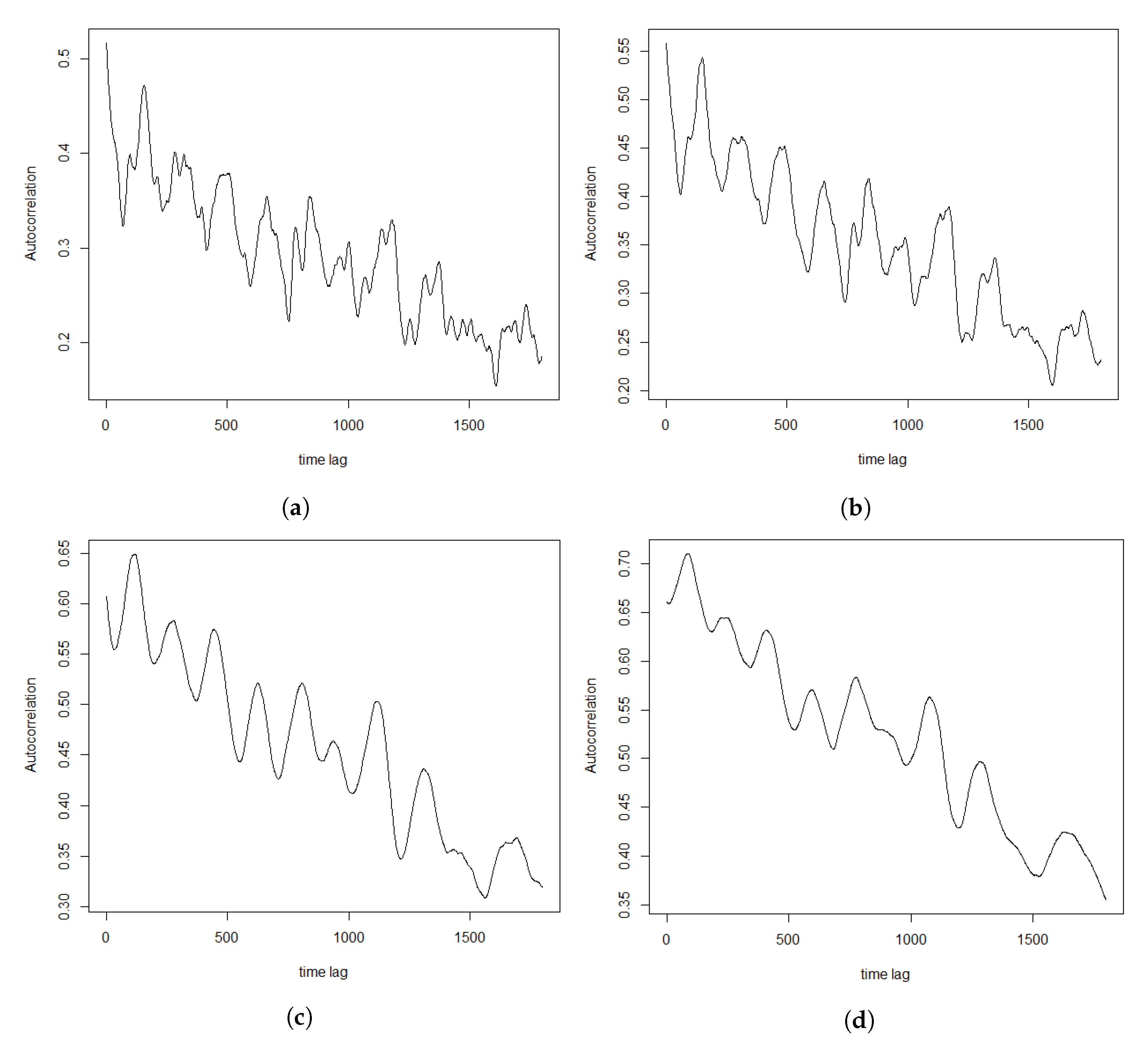
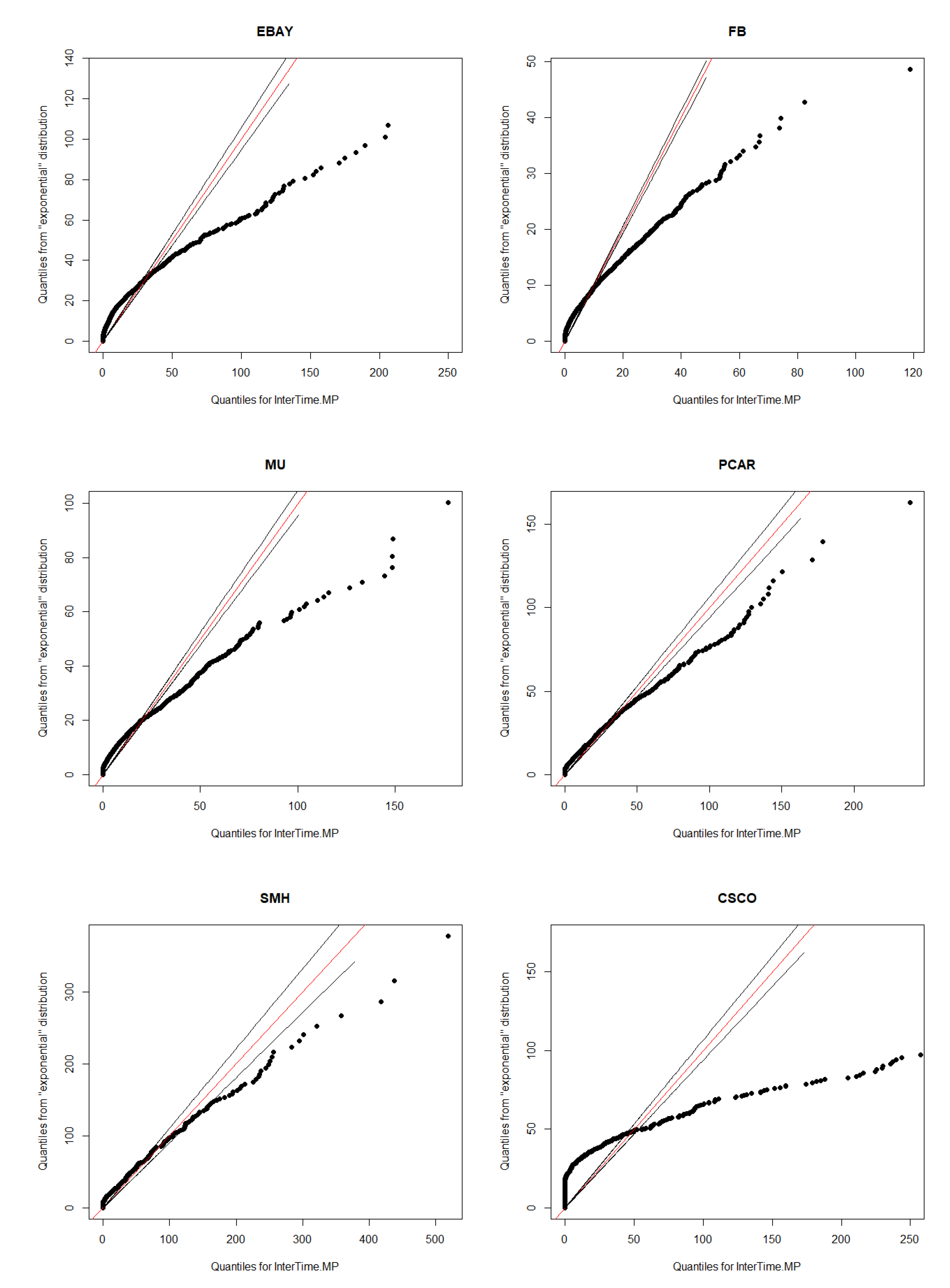
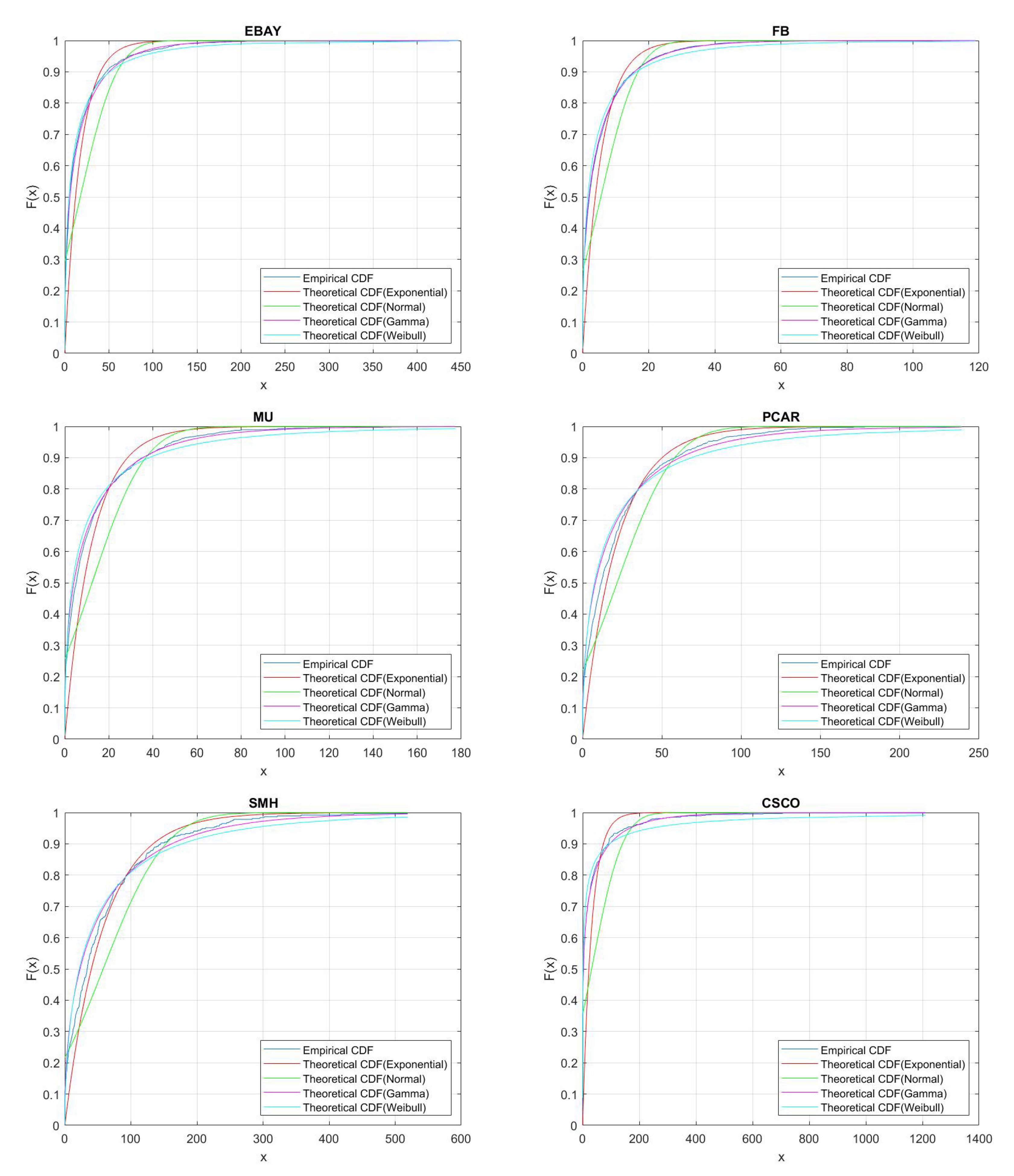
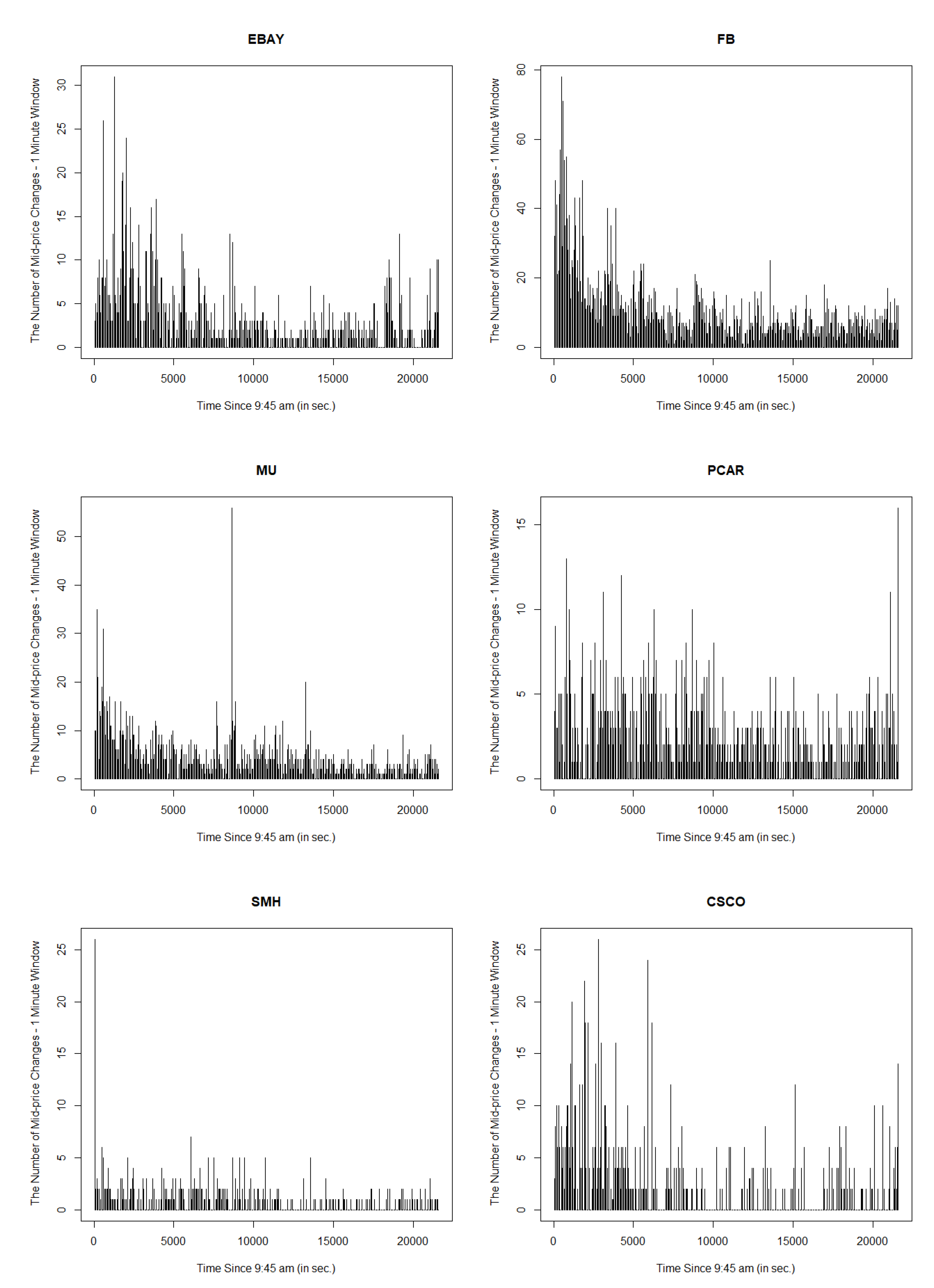
Section 3, including data and their clustering features descriptions, QQ-plots and autocorrelations. Section 4 presents Hawkes process and different models’ parameters calibration’s results. Error measurements and comparative analysis are considered in Section 5. Section 6 concludes the paper.

2. Theoretical Analysis

2.1. One-Dimensional Hawkes Process

2.1.1. Definition

The one-dimensional Hawkes Process is a point process N ( t ) which is characterized by its intensity function λ ( t )
λ ( t ) = h ( λ + 0 t μ ( t s ) d N ( s ) )
where the constant λ is called the background intensity and the function μ ( · ) is called the excitation function that satisfies 0 μ ( s ) d s < 1 . In Equation (1), if h ( · ) is a non-linear function, then we call this Hawkes Process as One-dimensional Non-linear Hawkes Process.
Typically, in this paper, the point process N ( t ) is represented as the cumulative number of mid-price changes up to current time t in the trading system. h ( · ) is set to be a linear function, that is, h ( x ) = x , and μ ( · ) is set to be an exponential function, that is, μ ( t ) = α e β t . This typical setting is widely used in most of the academic research (see Laub et al. 2015). Therefore, in this paper, the intensity function of the One-dimensional Hawkes Process is
λ ( t ) = λ + 0 t α e β ( t s ) d N ( s )

2.1.2. Calibration

In this paper, Maximum Likelihood Estimation (MLE) is used for calibration of the One-dimensional Hawkes Process. Suppose that the Hawkes process is observed over some time period [ 0 , T ] [ 0 , t k ] . Then, the log-likelihood function of Hawkes process is (see References Laub et al. 2015; Lorenzen 2012),
l = i = 1 k log [ λ + α j = 1 i 1 e β ( t i t j ) ] λ t k + α β i = 1 k [ e β ( t k t i ) 1 ]
If we let A ( i ) = j = 1 i 1 e β ( t i t j ) , for i = { 2 , 3 , , k } , and A ( 1 ) = 0 , then Equation (3) can be transformed into
l = i = 1 k log [ λ + α A ( i ) ] λ t k + α β i = 1 k [ e β ( t k t i ) 1 ]
However, in this case, the log-likelihood function is difficult to be solved manually and thus we need to use some computational methods (e.g., Partical Swarm Optimization (PSO)) to find the global optimization of the parameters λ , α , β .

2.2. General Compound Hawkes Process

2.2.1. Definition

Compound Poisson Process is a widely used model in risk management and finance, with some independently arriving jumps that follow the Poisson Process,
S t = S 0 + k = 1 N ( t ) a ( X k ) .
In this model, N ( t ) is a Poisson Process, X k is a continuous time n-state Markov Chain; a ( X k ) is a continuous and bounded mapping function on the state space X : = { 1 , 2 , , n } . If we change the model a little bit, we can get our new General Compound Hawkes Process
S t = S 0 + k = 1 N ( t ) a ( X k )
where N ( t ) is a one-dimensional Hawkes Process with the intensity function mentioned in Equation (2). In our case, this model is used for mid-price modelling and thus N ( t ) represents the number of mid-price changes up to time t; a ( X k ) represents the price movements interval. As we can see, models (5) and (6) look the same at first sight but they are different with respect to N ( t ) : in (5) it is the Poisson process and in (6) it is the Hawkes process.
From general to typical cases, if X k is an n-state Markov Chain, this model is called the General Compound Hawkes Process with n-state Dependent Orders (GCHPnSDO); if X k is a 2-state Markov Chain, this model is called the General Compound Hawkes Process with 2-state Markov Chain (GCHP2SDO); if in the 2-state Markov Chain, the value of a ( X k ) is set to be the most typical case, that is, the value of a ( X k ) is fixed, a ( X k ) = δ or a ( X k ) = δ , then this model is called the General Compound Hawkes Process with Dependent Orders (GCHPDO).

2.2.2. Diffusive Limit

Let X k be an ergodic n-state Markov Chain with state space X : = { 1 , , n } , that is, X k = { 1 , 2 , , n } and with ergodic probabilistic ( π 1 * , π 2 * , , π n * ) ; S t is defined in GCHPnSDO model. The diffusive limit of GCHPnSDO is derived in Reference Swishchuk and Huffman (2018),
S n t N ( n t ) a ^ * n n σ ^ * λ / ( 1 μ ^ ) W ( t )
where W ( t ) is a standard Wiener Process,
0 < μ ^ : = 0 μ ( s ) d s = α β < 1
0 s μ ( s ) d s <
a ^ * : = i X π i * a ( i )
σ ^ * : = i X π i * v ( i ) v ( i ) = b ( i ) 2 + j X ( g ( j ) g ( i ) ) 2 P ( i , j ) 2 b ( i ) j X ( g ( j ) g ( i ) ) P ( i , j ) b ( i ) : = a ( i ) a * b = ( b ( 1 ) , b ( 2 ) , , b ( n ) ) g : = ( P + Π I ) 1 b
In Equation (11), P denotes the transition probability matrix of the Markov Chain, that is, P ( i , j ) = P ( X k + 1 = j X k = i ) ; Π * denotes the matrix of stationary distribution of the Markov Chain. When the power n of the transition probability matrix P is large enough, P n n Π * , and all rows of Π * will be the same.
The diffusive limit of GCHP2SDO and GCHPDO model can still use Equation (7) since they are the typical cases of GCHPnSDO model. In Section 3, we will further introduce how to use the diffusive limit to estimate the correctness of the mid-price modelling by the General Compound Hawkes Process.

3. Application

3.1. Limit Order Book

A Limit Order Book (LOB) is just like a book that records financial big data in the market. Here, we consider two types of tradings, one is called market order (buy/sell) and the other one is called limit order (buy/sell). In the trading system, market order will be executed immediately when it arrives; limit order will wait for later execution and while waiting it can be cancelled. Therefore, limit order book is a collection of queued active limit orders awaiting execution or cancellation (see Gould et al. 2013).
Then we will give some definitions in Limit Order Book. Lot size means the smallest amount of the asset that can be traded within LOB. Tick size means the smallest permissible price interval between different orders within LOB (e.g., Suppose that the tick size in the trading system is 1 cent. Then, all the orders should be submitted in the exactly two decimal places). Bid price means the highest stated price among active buy orders at time t. Ask price means the lowest stated price among active sell orders at time t. Mid price is the price between the bid and ask price, that is,
M i d P r i c e = B i d P r i c e + A s k P r i c e 2

3.2. Data

One remark should be made with respect to the choice of real data. In different papers we used different types of real data—LOBster (five stocks Amazon, Apple, Google, Intel, Microsoft on 21 June 2012), 15 stocks from Deutsche Boerse Group (23 September 2013) and CISCO asset (3 November 2014) in References Chavez-Casillas et al. (2019); Swishchuk and Vadori (2017); Swishchuk et al. (2017), respectively, to justify and illustrate our approach.
In the present paper, we decide to use another set of real data, namely EBAY, FB, MU, PCAR, SMH, CSCO, (provided by Reference Cartea et al. (2015), book), to check our methods and to justify and illustrate our approach, and as in our previous papers, the outcomes of the present paper show that the method is right and gives very good results.
Thus, in this paper, the real LOB data of EBAY, FB, MU, PCAR, SMH is downloaded from http://sebastian.statistics.utoronto.ca/books/algo-and-hf-trading/data/. What we get from this link is a zip file with matlab data from November 2014 for the following tickers—AMZN, EBAY, FB, GOOG, INTC, MSFT, MU, PCAR, SMH, VOD for every second of the trading day. We reject the stocks that we tested in the previous papers. Each file contains a structure called LOB where each field has entries corresponding to one second of the trading day—NumberMO, volumeMO, EventTime, BuyPrice, SellPrice, BuyVolume, SellVolume, MO. Moreover, the real LOB data of CSCO is downloaded from https://sites.google.com/site/algorithmictradingbook/website-builder. What we get from this link is a zip file with matlab data from 3 November 2014 to 7 November 2014. Each file contains a structure called data with five elements—Event, SellVolume, SellPrice, BuyVolumne, BuyPrice.
We randomly choose 1 day in November to see how our models work on these stocks. For the mid price modelling in Section 4.2, the data files we use in this paper are EBAY_20141110, FB_20141110, MU_20141110, PCAR_20141110, SMH_20141110, CSCO_20141107. Consider for each trading day, it starts from 9:30 and ends at 16:00. In order to avoid the open and close auctions, we ignore the first and last 15 min, and thus we end with 6 trading hours per day, between 9:45 and 15:45. The number of mid price changes in a day for EBAY, FB, MU, PCAR, SMH, CSCO are 1255, 3988, 1756, 1008, 379, 943.

3.3. Descriptive Data Analysis

Before we will work with our new General Compound Hawkes Process Model, we need to check the following questions first. Comparing with the Compound Poisson Process, we want to know whether we could reject Poisson process; furthermore, we want to know whether there is a correlation between the mid-price changes. After that, we plot the number of arrivals under a fixed time window to explore these features in the real data.

3.3.1. QQ-Plot

In Figure 1, the QQ-plot rejects Poisson Process since the inter-arrival time does not follow the exponential distribution. In Figure 1, the two black straight lines are the confidence boundary under 95% confidence level; the red straight line is y = x . If the inter-arrival time of the mid price changes follow the exponential distribution, all the black points should approximately be on the red line, within the confidence boundary. However, from the Figure 1, it is obvious to reject this assumption.
Furthermore, if the exponential distribution does not fit the inter-arrival times well, we want to know which distribution will fit better. We tried normal distribution, Gamma distribution, Weibull distribution, and then compared the theoretical Cumulative Density Function (CDF) with the empirical CDF (See Figure 2). From Figure 2, it is obvious that in most cases, Gamma or Weibull distribution performs much more better than the others since the curve of the theoretical CDF nearly coincides with that of empirical CDF.
Of course, quantitative measures can be used as well to compare the different models, such as MLE of the Weibull and Gamma distributions’ parameters as we did in Reference Swishchuk and Vadori (2017), for LOBster data or in Reference Chavez-Casillas et al. (2019), for Facebook data. However, we gave here two different visualized comparisons, namely Q Q -plots and CDFs, for 6 different stocks to illustrate our approach which proved to be right.

3.3.2. Autocorrelation

To further confirm that the mid price changes are not independent, we calculated the autocorrelation by using equation
C ( τ , δ ) = E [ ( N t + τ N t ) ( N t + 2 τ + δ N t + τ + δ ) ] E [ ( N t + τ N t ) ] E [ ( N t + 2 τ + δ N t + τ + δ ) ] v a r ( N t + τ N t ) v a r ( N t + 2 τ + δ N t + τ + δ )
where τ is the length of the time interval, δ is the time lag, that is, the length between two consecutive time intervals. In Equation (13), if τ is fixed, then the autocorrelation function C ( τ , δ ) will become a function that is respective to δ , that is, C ( δ ) . Take FB20141110 data as example. In the four plots shown in Figure 3, the length of the time interval is changed, (a) τ = 20 s, (b) τ = 30 s, (c) τ = 60 s, (d) τ = 90 s. In each graph, the X-coordinate represents the time lag δ which is changed from 1 s to 30 min by a step of 1 s.
From Figure 3, it is obvious to see that the shape of the autocorrelation function are nearly identical even if the plot is noisier when τ decreases. Moreover, something more interesting could also be discovered from Figure 3. Even if δ = 30 min, the value of the correlation function in each plot is still above 0.2 which is not neglectable. This means that suppose there is an arrival of mid price change at current time t and then the impact of this arrival will last more than 30 min in the trading system, which is much longer than we can imagine.

3.3.3. Clustering Feature

At the end of the Descriptive Data Analysis, we plot the number of mid price changes occurring in every minute during the trading day. The clustering feature is obvious to be discovered in Figure 4.
From Section 3.3.1, Section 3.3.2, Section 3.3.3, the main conclusion that we can make is trading activities are not a completely random and memoryless process.

4. Hawkes Process and Models Calibrations

In this section we calibrate Hawkes process’ parameters λ , α , β (Section 4.1) and our mid-price S t model’s parameters a ( 1 ) , , a ( n ) (Section 4.2) for different GCHP (see (Section 4.2.1, Section 4.2.2, Section 4.2.3) to find the price’s volatility σ * λ / ( 1 α / β ) , obtained in (7). To estimate the models fitting accuracy, we define in Section 5 an error rate for each model, and set the threshold value as 15 % . The model with error rate less than the threshold is considered as well fitted. Thus, we define which of the models is the best fit for which real data.

4.1. Hawkes Process’ Parameters Calibration

The Particle Swarm Optimization (PSO) method is used to solve the log-likelihood function in Equation (4) and find the global optimization of the parameters λ ^ , α ^ , β ^ . If the calibration result is appropriate, E [ N ( [ 0 , 1 ] ) ] λ ^ 1 α ^ β ^ (see Laub et al. 2015), where E [ N ( [ 0 , 1 ] ) ] is the empirical expectation of the number of mid price changes arriving in a unit time interval.
From Table 1, it is obvious to see that the values in the last two columns are super close, which means that our parameter estimation is appropriate.

4.2. Mid Price Modelling and Calibration

After Section 4.1, we can successfully model N ( t ) , the cumulative number of mid price changes up to current time t. Then, in this section, we will move forward to the mid price modelling by General Compound Hawkes Process. We will start from the most typical GCHPDO model and then move forward to the most general GCHPnSDO model. Under each model, the most important thing to figure out is the value of a ( X k ) .

4.2.1. GCHPDO

In the case of GCHPDO model, the value of a ( X k ) can only take the fixed number. Suppose that X k { δ , δ } and a ( x ) = x , that is, a ( X k ) = δ or a ( X k ) = δ , where δ is the tick size of mid price in the trading system. In our case, suppose the tick size in the trading system is 1 cent. Whenever the ask/bid price goes up/down by 1 cent, the mid price will go up/down by 0.5 cent. Therefore, the tick size of the mid price movement is 0.5 cent.
Rearrange the Equation (7),
S n t N ( n t ) a ^ * n σ ^ * n λ ^ 1 α ^ β ^ W ( t )
From 9:45 a.m. to 15:45 p.m., cut this 6 trading hours into some disjoint windows of size n, with t = 1 , that is, the disjoint time intervals are [ i n , ( i + 1 ) n ] . Then, the left hand side of Equation (14) can be discretized into
S i * = ( S ( i + 1 ) n S i n ) ( N ( ( i + 1 ) n ) N ( i n ) ) a ^ *
Combining Equations (14) and (15), a converging formula between the standard deviation and its theoretical counterpart can be received,
s t d { S i * } n σ ^ * n t λ ^ 1 α ^ β ^ , t = 1
By (16), we can use this to estimate the correctness of the model fitting. If our model fitting is perfect, then
s t d { S i * } σ ^ * n λ ^ 1 α ^ β ^
Figure 5 shows the empirical standard deviation against its theoretical counterpart for various window sizes, starting from 10 s to 20 min by the step of 10 s. Except for the CSCO result, it is obvious to see that the differences between the empirical standard deviation and its theoretical counterpart are kind of large in the rest of five stocks. The reason for these unsatisfying results is that GCHPDO model assumes at each change, the mid price can only go up/down by tick size = 0.05 cent. However, in reality, only a small percentage of mid price movements change in this way (see Table 2).

4.2.2. GCHP2SDO

According to Section 4.2.1, GCHPDO is too special to model the mid price movements of stocks EBAY, FB, MU, PCAR, and SMH, and thus we need to consider some more general models. In GCHP2SDO model, the way we determine the value of a ( X k ) depends on the real data rather than just on the trading system. Take the mean of the upward and downward mid price movements and then assign them to a ( 1 ) and a ( 2 ) . The result in Table 3 shows that in GCHP2SDO model, the mid price does not go up/down by exactly 0.5 cent at each change, which leads the model fitting to become much better than the GCHPDO model (see Figure 6).

4.2.3. GCHPnSDO

For upward or downward mid price movement, the above GCHPDO and GCHP2SDO models only consider 1 possible price interval since X k is only a 2-state Markov Chain. In this section, we are trying to figure out whether there is more than 1 possible price interval that could better fit the mid price movements than GCHP2SDO model.
Firstly, we need to figure out a way to determine the value of a ( X k ) . Step1: After calculating the mid price changes, we separate the data into upward and downward movements. Step 2: we calculate the (evenly/unevenly) distributed quantiles for both data sets. Depending on the data, several quantiles may be identical and then we reject any duplicates. At the end of this step, we have gotten a list of bounds B k , which we will use for determine the value of a ( X k ) . Step 3: a ( X k ) = the average of all mid-price changes located between two neighbouring boundary values, that is, [ B k , B k + 1 ) . Step 4: There is an exception for the largest upper boundary, that is, after step 3, we will not get the value for a ( X n ) . And thus, we need to calculate the mean of the rest data manually and assign it to a ( X n ) .
Secondly, we need to determine the best n for GCHPnSDO model. For different stocks, the Mean Square Errors (MSE) between the empirical standard deviation and its theoretical counterpart under varied number of states are shown in Table 4, Table 5, Table 6, Table 7 and Table 8. We tried limited n, and then pick up the best n under the smallest MSE. For EBAY, the best GCHPnSDO model is the GCHP8SDO model; for FB, the best GCHPnSDO model is GCHP4SDO model; for MU, the best GCHPnSDO model is the GCHP4SDO model; for PCAR, the best GCHPnSDO model is the GCHP15SDO model; for SMH, the best GCHPnSDO model is the GCHP9SDO model.
In the end, compare the MSE of the best GCHPnSDO models with that of the previous GCHPDO and GCHP2SDO models. Again, pick up the best model for mid price movements under the smallest MSE (see Table 9). Under the best model, the model fitting results can be seen in Figure 7.

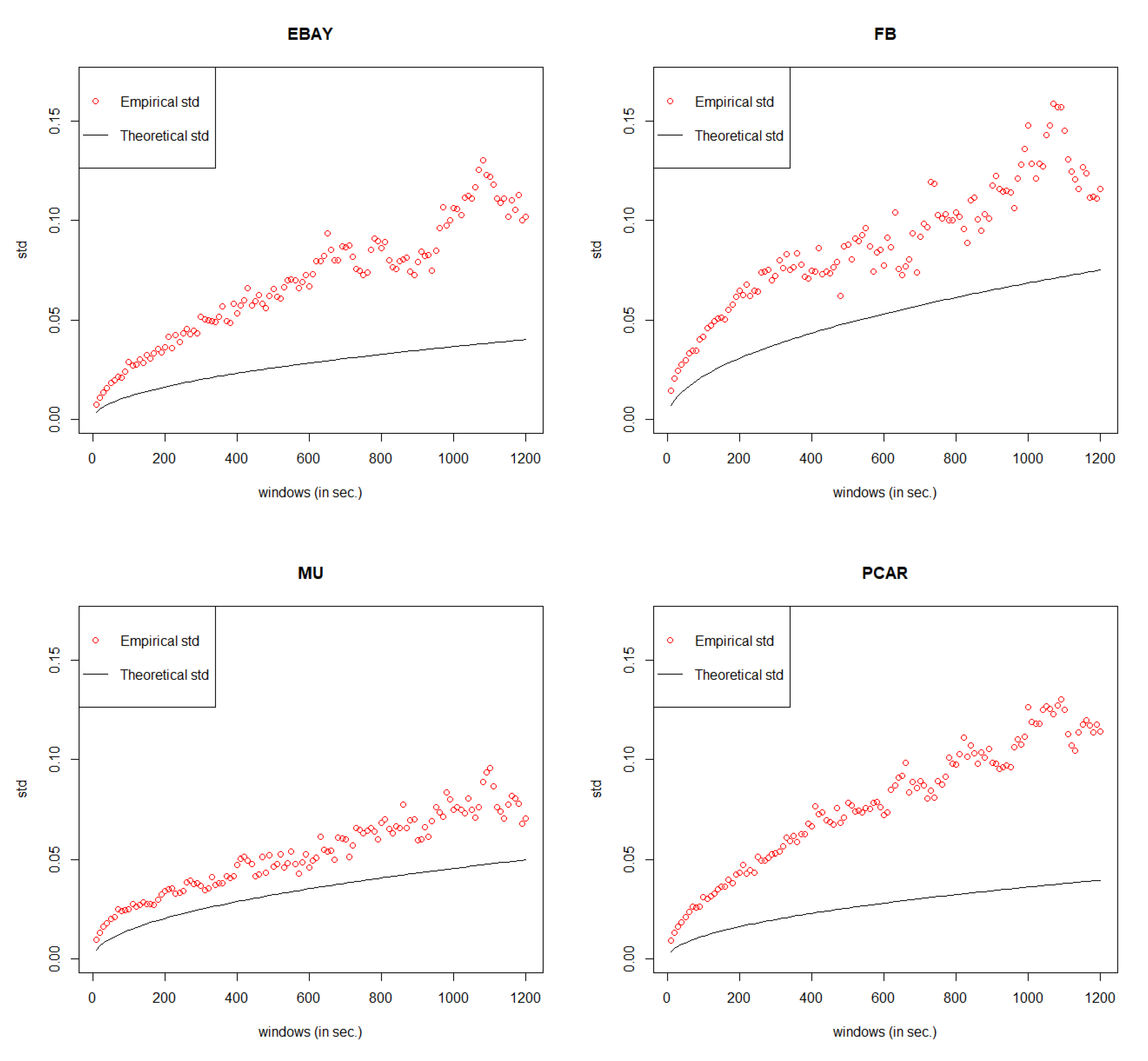
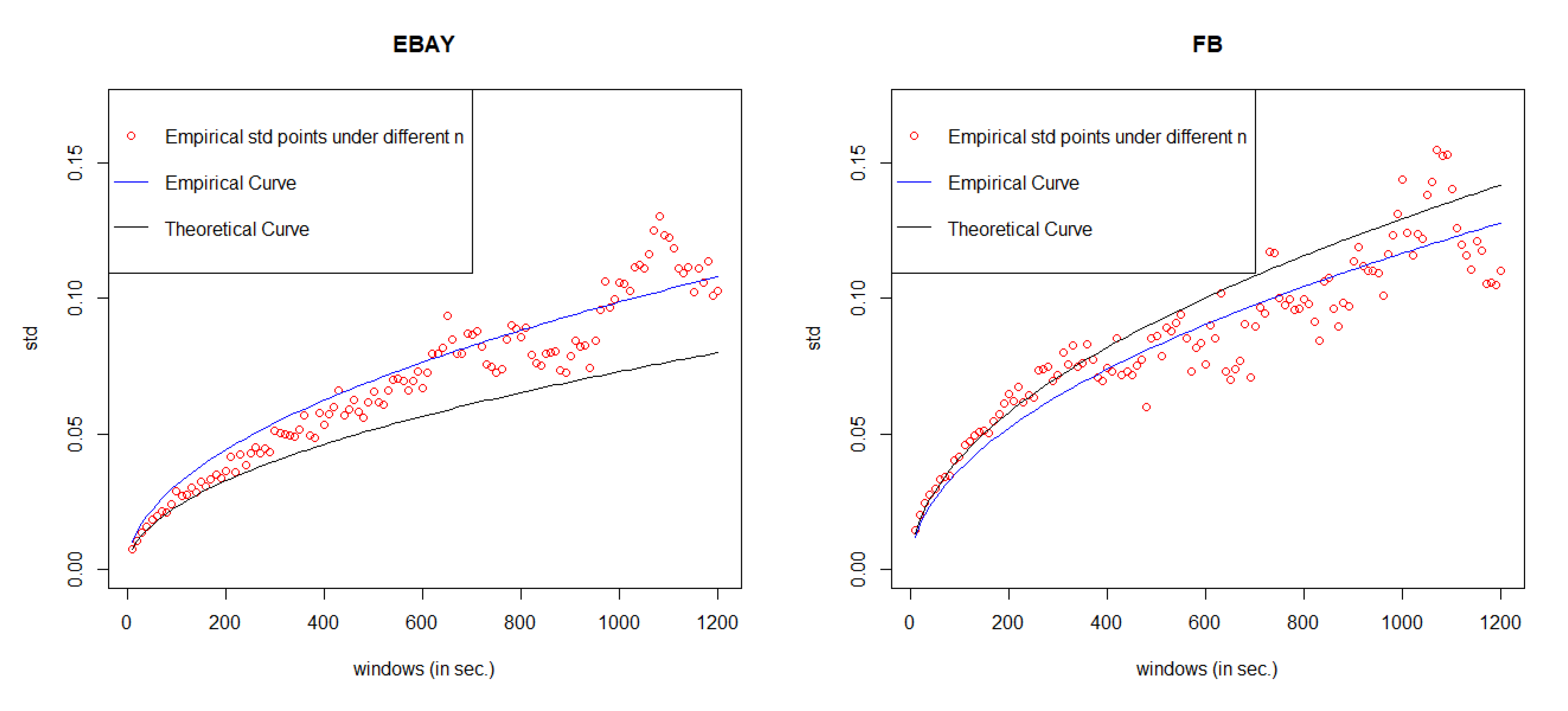
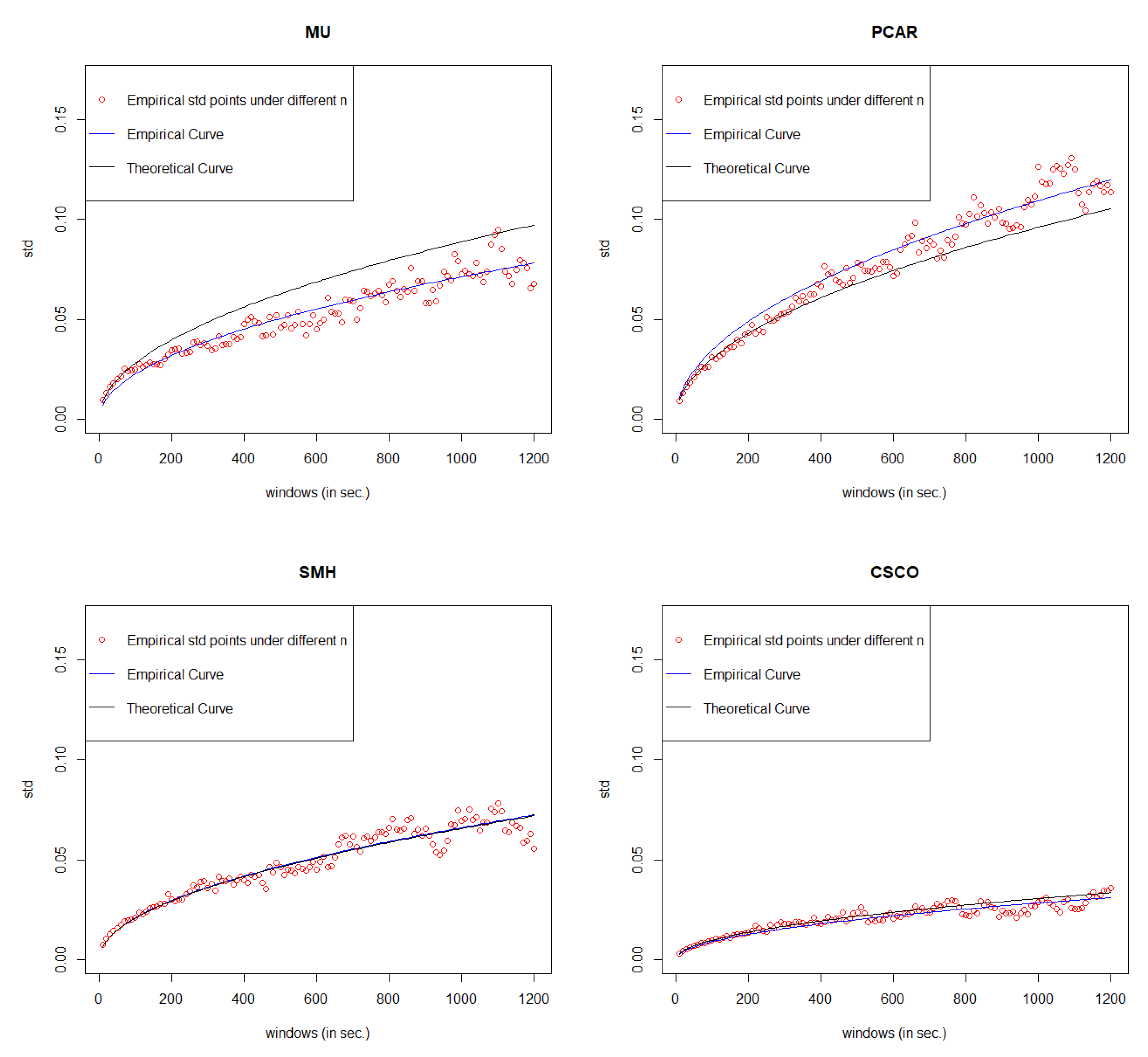
5. Error Measurement

Since the value of MSE is always very small under GCHPDO, GCHP2SDO, and GCHPnSDO models, it makes no sense to measure the correctness of model fitting under the best model only by MSE. Therefore, in this paper, we proposed a new way to measure the correctness. If we take the square of both sides in Equation (16), we can get
( s t d { S i * } ) 2 n ( ( σ ^ * ) 2 λ ^ 1 α ^ β ^ ) n t , t = 1
Equation (18) means that when n goes to infinity, the square of s t d { S i * } converges to a linear regression function L 1 = ( ( σ ^ * ) 2 λ ^ 1 α ^ β ^ ) n with respective to n. Therefore, based on the real points ( s t d { S i * } ) 2 under different n, we can estimate the linear regression function L = c n by least square method, where c is the estimated slope. Then, we take the square root of estimated function L , we can get our estimated curve of s t d { S i * } . The comparison between the empirical curve and the theoretical curve is shown in Figure 8.
Under the best model, the error rate of each stock is listed in Table 10. If we set the threshold value as 15%, the model with error rate less than threshold can be considered as well fitted. Table 10 shows that our General Compound Hawkes Process correctly models the mid price movements of 4 stocks among 6.
We define the error rate as
c σ ^ * λ ^ 1 α ^ β ^ c × 100 %
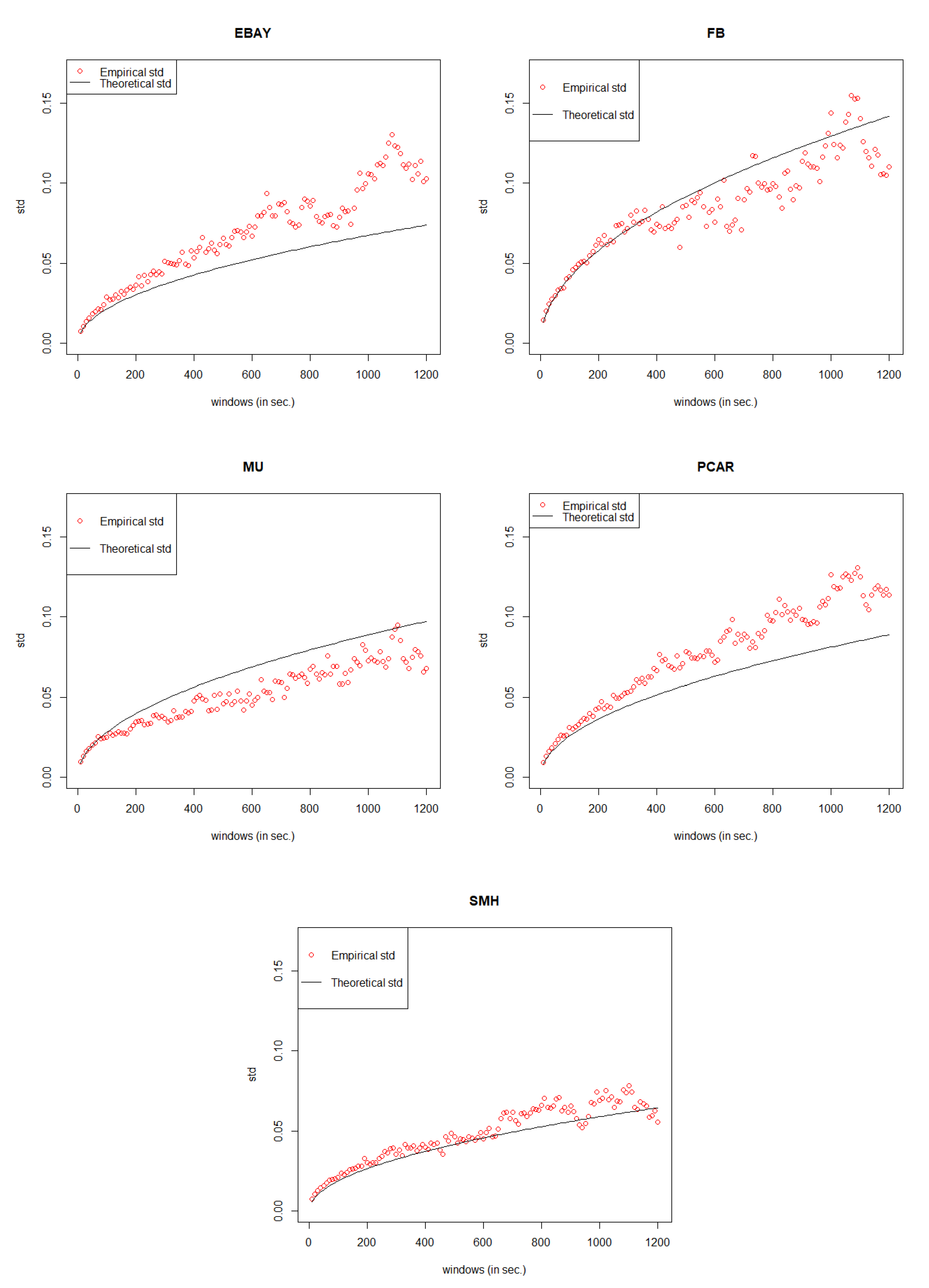
In order to avoid any bias of data selection, we do the simulation again by following the same process mentioned in Section 3 to Section 5 to justify our General Compound Hawkes Processes work well not just for one day but also for other days. In the data set of EBAY, FB, MU, PCAR, SMH, we randomly choose the date 18 November 2014; for the data set of CSCO, we randomly choose the date 6 November 2014.
For descriptive data analysis, we have gotten the quite similar results as those shown in Figure 1, Figure 2, Figure 3 and Figure 4. Hawkes Process Calibration results are shown in Table 11.
Similarly, for CSCO data, since the intervals of price movements are always $0.5, the GCHPDO model should be the best fit. To find the best n of the GCHPnSDO model for EBAY, FB, MU, PCAR, SMH, we have tried limited n and then picked up the best n under the smallest MSE. From Table 12, Table 13, Table 14, Table 15 and Table 16, we can see that for EBAY, the best GCHPnSDO model is GCHP5SDO; for FB, the best GCHPnSDO model is GCHP4SDO; for MU, the best GCHPnSDO model is GCHP4SDO; for PCAR, the best GCHPnSDO model is GCHP4SDO; for SMH, the best GCHPnSDO model is GCHP6SDO.
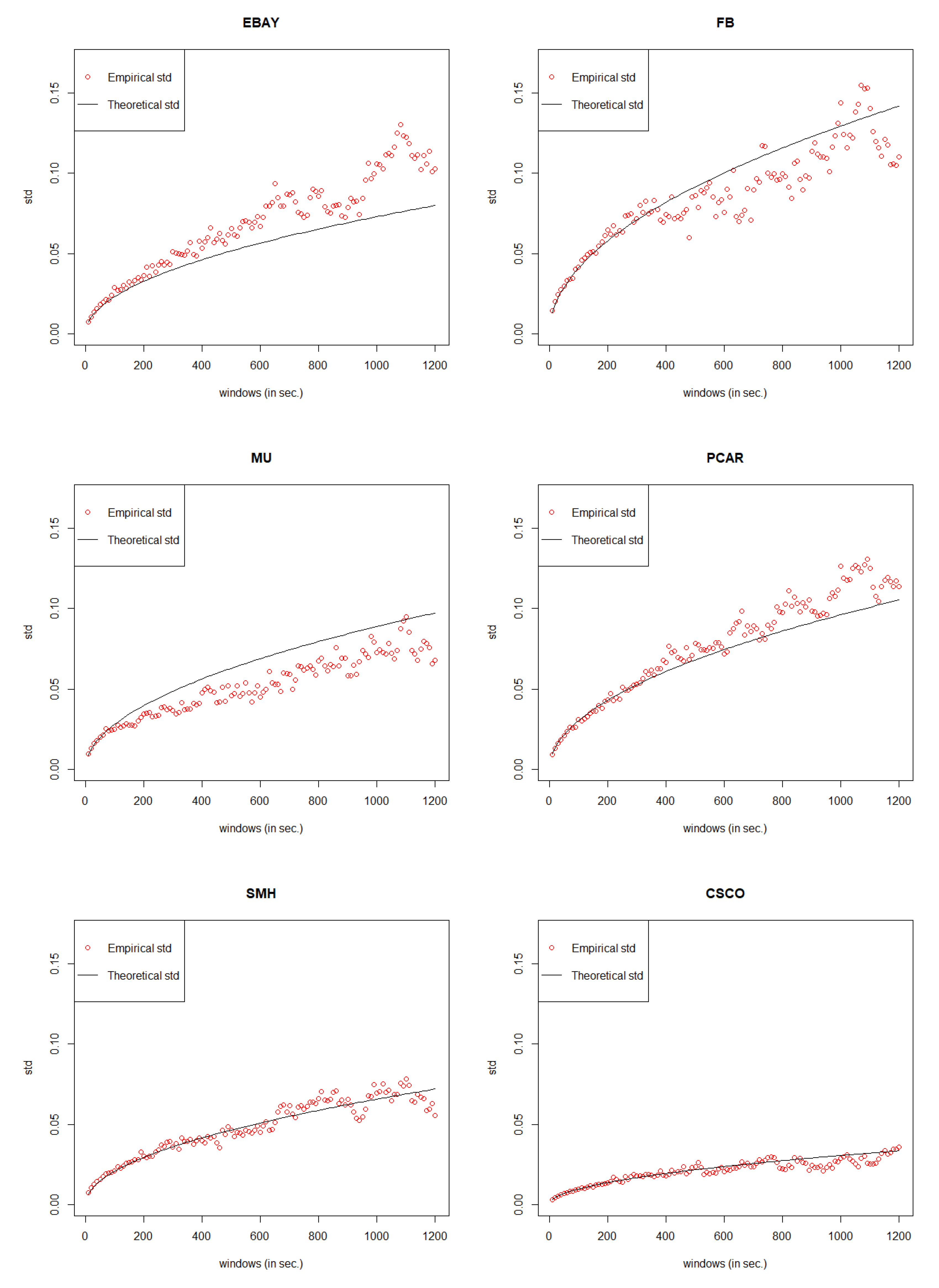
Compare the MSE of the best GCHPnSDO models with that of GCHPDO and GCHP2SDO models. Again, pick up the best model for mid price movements under the smallest MSE and then calculate the error rate following the same method derived in Equation (19). Within the error rate threshold of 15%, in Table 17, we could see that our General Compound Hawkes Processes successfully track the mid price movements of FB, MU, PCAR, SMH, and CSCO.

6. Conclusions and Future Work

The main contribution and novelty of the paper consists in introducing different new types of General Compound Hawkes Processes (GCHPDO, GCHP2SDO, GCHPnSDO) and their diffusive limits to model the mid price movements. Based on our previous research, we further expand our data sets to justify whether our models still work well on the stocks of EBAY, FB, MU, PCAR, SMH, CSCO (provided by Reference Cartea et al. (2015) book). We define the error rates to estimate the models fitting accuracy and set the threshold to 15%. Based on the data sets named EBAY_20141110, FB_20141110, MU_20141110, PCAR_20141110, SMH_20141110, CSCO_20141107, the best model for EBAY is GCHP8SDO; for FB, the best model is GCHP2SDO; for MU, the best model is GCHP2SDO; for PCAR, the best model is GCHP15SDO; for SMH, the best model is GCHP9SDO; for CSCO, the best model is GCHPDO. Under the best model, our General Hawkes Processes successfully track the mid price movements of 4 stocks out of 6. To further avoid any bias of data selection process, again, we randomly choose the data from another date in our data sets, and gain the quite similar results. Those results justify that our General Compound Hawkes Processes could be right and could be applied for the data not just from a specific day but also from other days.
The future work will be devoted to the prediction analysis with different models introduced in this paper, and justifications of those model using real data.

Author Contributions

Q.H.: software, validation, data curation, visualization, writing—original draft preparation. A.S.: project administration, supervision, writing—review and editing, conceptualization, methodology.

Funding

This research received no external funding.

Conflicts of Interest

The authors declare no conflict of interest.

References

  1. Bacry, Emmanuel, Sylvain Delattre, Marc Hoffmann, and Jean-Francois Muzy. 2013. Some limit theorems for hawkes processes and application to financial statistics. Stochastic Processes and their Applications 123: 2475–99. [Google Scholar] [CrossRef]
  2. Bacry, Emmanuel, Iacopo Mastromatteo, and Jean-François Muzy. 2015. Hawkes processes in finance. arXiv. [Google Scholar]
  3. Cartea, Álvaro, Sebastian Jaimungal, and José Penalva. 2015. Algorithmic and High-Frequency Trading. Cambridge: Cambridge University Press. [Google Scholar]
  4. Chavez-Casillas, Jonathan, Robert J. Elliott, Bruno Remillard, and Anatoliy V. Swishchuk. 2019. A level-1 limit order book with time dependent arrival rates. Methodology and Computing in Applied Probability 21: 699–719. [Google Scholar] [CrossRef]
  5. Cont, Rama, and Adrien De Larrard. 2013. Price dynamics in a Markovian limit order markets. SIAM Journal on Financial Mathematics 4: 1–25. [Google Scholar] [CrossRef]
  6. Da Fonseca, José, and Riadh Zaatour. 2013. Hawkes process: Fast calibration, application to trade clustering, and diffusive limit. Journal of Futures Markets 34: 548–79. [Google Scholar] [CrossRef]
  7. Embrechts, Paul, Thomas Liniger, and Lu Lin. 2011. Multivariate hawkes processes: An application to financial data. Journal of Applied Probability 48: 367–78. [Google Scholar] [CrossRef]
  8. Gould, Martin D., Mason A. Porter, Stacy Williams, Mark McDonald, Daniel J. Fenn, and Sam D. Howison. 2013. Limit order books. Quantitative Finance 13: 1709–42. [Google Scholar] [CrossRef]
  9. Hawkes, Alan G. 1971. Spectra of some self-exciting and mutually exciting point processes. Biometrika 58: 83–90. [Google Scholar] [CrossRef]
  10. Laub, Patrick J., Thomas Taimre, and Philip K. Pollett. 2015. Hawkes Processes. arXiv. [Google Scholar]
  11. Lorenzen, Florian. 2012. Analysis of Order Clustering Using High Frequency Data: A Point Process Approach. Ph.D. thesis, Swiss Federal Institute of Technology Zurich (ETH Zurich), Zurich, Switzerland. [Google Scholar]
  12. Swishchuk, Anatoliy, and Aiden Huffman. 2018. General Compound Hawkes Process in Limit Order Books. arXiv. [Google Scholar]
  13. Swishchuk, Anatoliy, and Nelson Vadori. 2017. A semi-Markovian modeling of limit order markets. SIAM Journal on Financial Mathematics 8: 240–73. [Google Scholar] [CrossRef]
  14. Swishchuk, Anatoliy, Tyler Hofmeister, Katharina Cera, and Julia Schmidt. 2017. General semi-Markov model for limit order books. International Journal of Theoretical and Applied Finance 20: 1750019. [Google Scholar] [CrossRef]
  15. Swishchuk, Anatoliy, Bruno Remillard, Robert Elliott, and Jonathan Chavez-Casillas. 2019. Compound Hawkes processes in limit order books. In Financial Mathematics, Volatility and Covariance Modelling, 1st ed. Edited by Julien Chevallier, Goutte Stéphane, Guerreiro David, Saglio Sophie and Bilel Sanhaji. Abingdon: Routledge, vol. 2. [Google Scholar]
  16. Zhou, Ke, Hongyuan Zha, and Le Song. 2013. Learning triggering kernels for multi-dimensional hawkes processes. Paper presented at the 30th International Conference on Machine Learning, PMLR, Atlanta, GA, USA, June 16–21; vol. 29, pp. 1301–9. [Google Scholar]
Figure 1. QQ-plot for 6 different stocks.
Risks 07 00110 g001
Figure 2. CDF comparison between different distributions.
Risks 07 00110 g002
Figure 3. Autocorrelation under different τ . (a) τ = 20 s. (b) τ = 30 s. (c) τ = 60 s. (d) τ = 90 s.
Risks 07 00110 g003
Figure 4. Clustering features for 6 different stocks.
Risks 07 00110 g004
Figure 5. General Compound Hawkes Process with 2 fixed Dependent Orders model fitting results.
Risks 07 00110 g005aRisks 07 00110 g005b
Figure 6. General Compound Hawkes Process with 2 non-fixed Dependent Oorder model fitting results.
Risks 07 00110 g006
Figure 7. Best model fitting results for 6 stocks.
Risks 07 00110 g007
Figure 8. Error measurements for 6 stocks.
Risks 07 00110 g008aRisks 07 00110 g008b
Table 1. Calibration Result of Hawkes Process.
Stock λ ^ α ^ β ^ E [ N ( [ 0 , 1 ] ) ] λ ^ 1 α ^ β ^
EBAY0.0514296424.16091427208.3614110.0581693960.05817548
FB0.14607577.036856433.63547580.1847088150.184721079
MU0.066857768.4926784247.386558650.0814463610.081456495
PCAR0.0410556728.42153021234.18784090.0467201010.046726496
SMH0.015773610.6972559102.69088890.0176023980.017607795
CSCO0.0223269642.63914601311.86845730.0436574070.043766646
Table 2. Tick-size rate.
StockTick-Size Rate
EBAY21.35%
FB18.18%
MU9.85%
PCAR22.22%
SMH12.96%
CSCO100%
Table 3. a ( X k ) for GCHP2SDO.
Stock a ( 1 ) a ( 2 )
EBAY0.0091730474−0.0092358804
FB0.0095449949−0.0093280239
MU0.0098359729−0.0096846330
PCAR0.0116390041−0.0108269962
SMH0.0152972973−0.0134196891
Table 4. n Selection for EBAY.
n45678
MSE0.000467010.0004187030.0003993110.0003978980.000393683
Table 5. n Selection for FB.
n45678
MSE0.0003176330.0003300580.0003446560.0003490870.000361214
Table 6. n selection for MU.
n468
MSE0.0002635880.0002722370.000275675
Table 7. n selection for PCAR.
n691215
MSE0.0002381850.0001322240.0001292380.000124427
Table 8. n selection for SMH.
n67910
MSE0.000038534630.000034361680.000023959920.00002475711
Table 9. Model comparison.
StockGCHPDO (MSE)GCHP2SDO (MSE)GCHPnSDO (MSE)Best Model
EBAY0.0022009960.0005663050.000393683GCHP8SDO
FB0.001732830.0002413540.000317633GCHP2SDO
MU0.0004502420.0002276040.000263588GCHP2SDO
PCAR0.0031292170.0004681040.000124427GCHP15SDO
SMH0.0014773080.0000534740.00002395992GCHP9SDO
Table 10. Error rate under the best model.
StockError Rate
EBAY26.05%
FB10.95%
MU24.42%
PCAR12.18%
SMH0.67%
CSCO7.99%
Table 11. Calibration Result of Hawkes Process.
Stock λ ^ α ^ β ^ E [ N ( [ 0 , 1 ] ) ] λ ^ 1 α ^ β ^
EBAY0.03738607911.0671867577.585649540.043564810.043606288
FB0.163615319.4996209642.482370190.2104166670.210739442
MU0.0598900349.76771013765.909389640.0702777770.070309895
PCAR0.0303275710.8894463182.448066270.0348611110.034942673
SMH0.0158058141.96535566351.02217070.017870370.017952006
CSCO0.022357326677.55040081385.2154040.043379630.04376324
Table 12. n Selection for EBAY.
n4567
MSE0.0001549260.0001514770.0001826620.000193251
Table 13. n Selection for FB.
n4567
MSE0.0002047290.0002117060.0002413390.000249355
Table 14. n Selection for MU.
n468
MSE0.0000312050.0000323040.000038158
Table 15. n Selection for PCAR.
n46810
MSE0.0001431160.0001549220.0001620160.00032631
Table 16. n Selection for SMH.
n467910
MSE0.0000636410.0000512740.0000779540.0001028040.00010632
Table 17. Model comparison.
StockGCHPDO (MSE)GCHP2SDO (MSE)GCHPnSDO (MSE)Best ModelError Rate
EBAY0.0003957750.0000701190.000151477GCHP2SDO15.67%
FB0.0029795620.0001646280.000204729GCHP2SDO4.15%
MU0.0006914220.0000272260.000031205GCHP2SDO1.52%
PCAR0.0012201030.0000757080.000143116GCHP2SDO6.75%
SMH0.0010583990.0000768670.000051274GCHP6SDO4.21%
CSCO0.000020788N/AN/AGCHPDO13.29%

