High Frequency Price Change Spillovers in Bitcoin Markets

Abstract

The study of connectedness is key to assess spillover effects and identify lead-lag relationships among market exchanges trading the same asset. By means of an extension of Diebold and Yilmaz (2012) econometric connectedness measures, we examined the relationships of five major Bitcoin exchange platforms during two periods of main interest: the 2017 surge in prices and the 2018 decline. We concluded that Bitfinex and Gemini are leading exchanges in terms of return spillover transmission during the analyzed time-frame, while Bittrexs act as a follower. We also found that connectedness of overall returns fell substantially right before the Bitcoin price hype, whereas it leveled out during the period the down market period. We confirmed that the results are robust with regards to the modeling strategies.

1. Introduction

The study of connectedness is a key topic arising in the field of financial econometrics. As Diebold and Yilmaz (2009) state, connectedness features in important aspects of market risk, i.e., portfolio concentration and return connectedness, credit risk—default connectedness, systemic risk, that is system-wide connectedness, counter-party risk—, and bilateral and multilateral contractual connectedness, as well as business cycle risk, with intra- and inter-country real activity connectedness.

In particular, throughout the study of return and volatility, connectedness of financial assets is able to retrieve system-wide and pairwise connectedness measures that are useful to assess the systemic risk of financial groups and/or single entities. Furthermore, the study of directional connectedness is able to shed light on which are leading assets in terms of shock transmission and, rather, which are those that follow others in the process. This contributes to the stream of econometric literature studying price discovery.

However, in the financial literature there is a lack of studies exploring interconnectedness related to the same asset traded on different exchange platforms. Indeed, it is widely known that prices of the same good traded on different venues may consistently vary across exchange markets and that this is possibly due to lead-lag relationships existing across exchanges. This paper aims to fill this gap, as the study of system-wide connectedness can give insights on how much different trading platforms are synchronized in terms of returns (and, therefore, market prices), as well as how the study of directional connectedness is able to shed light on the lead-lag relationship among exchange markets. Indeed, unlike previous studies, we explored dynamic return connectedness among different exchange markets trading the same good: Bitcoin.

The methodology we employed can be applied, without loss of generality, to the rest of the cryptocurrency market, as well as to other financial products. To illustrate, studying interconnectedness and price discovery on the same asset or commodity returns when traded on different exchange platforms might give some insights on where the price formation process takes primarily place. Moreover, this technique may be applied to highly integrated markets to effectively measure spillovers taking into account for the common stochastic trends driving the co-movement of the underlying variables, as it can be the case for spot and future markets.

2. Literature Review

Much research in the field of financial econometrics has dealt with how econometric connectedness measures development. To illustrate, Billio et al. (2012) built systemic risk and econometric measures of interdependency which are suitable to be used in the finance and insurance sectors. Diebold and Yilmaz (2012) developed overall and directional measures for return and volatility spillovers which are built upon forecast error variance decompositions deriving from vector autoregressive models (VARs). In a related work, Diebold and Yilmaz (2014) extended their previously developed measures to a network topology representation of the forecast error variance decomposition, linking the econometric connectedness literature to that of financial networks. More recently and following the same approach, Baruník and Křehlík (2018) proposed a framework based on the spectral representation of variance decompositions to measure connectedness among financial variables which arise due to heterogeneous frequency responses.

Today, the existing literature focuses largely on measures applied to interconnectedness between financial entities belonging to different groups in terms of geography, financial sectors, etc. To illustrate, Diebold and Yilmaz (2013) studied the dynamics of global business cycle connectedness for a set of real output of six developed countries between 1962 and 2011. Demirer et al. (2018) studied the global bank equity connectedness linking the publicly-traded subset of the world’s top 150 banks during the period 2003–2014. Baruník et al. (2016) explored asymmetries in volatility spillovers that emerge due to bad and good volatility with the use of data regarding most liquid U.S. stocks across seven different sectors.

Since the birth of cryptocurrencies, a stream of literature started focusing on interconnectedness, spillover analyses and shock transmissions involving the cryptocurrency market. Fry and Cheah (2016) borrowed some modeling strategies from econophysics to study shocks and crashes in cryptocurrency markets and show that in the period of negative bubble there is a spillover from Ripple to Bitcoin. Yi et al. (2018) used a LASSO-VAR to estimate a volatility connectedness network linking as much as 52 different cryptocurrencies. Koutmos (2018) explored connectedness across 18 cryptocurrencies finding growing interdependencies among them. Corbet et al. (2018) analyzed dynamic volatility spillovers between traditional financial assets, such as gold, bond, equities, and the global volatility index (VIX) and three major cryptocurrencies, i.e., Bitcoin, Litecoin, and Ripple, through the Diebold and Yilmaz (2012) methodology, finding evidence of a relative isolation of the latter category with respect to the traditional ones. Using the same technique, Ji et al. (2019) studied connectedness across six large cryptocurrencies and showed that Litecoin and Bitcoin belong to the center of the connected network of returns, besides proving that connectedness is stronger via negative returns rather than via positive ones. Zięba et al. (2019) used, instead, minimum spanning trees (MSTs) to form cryptocurrency clusters and VAR models to examine the transmissions of demand shocks within clusters. They concluded that Bitcoin’s role, which was dominant until 2017, had then diminished, and they showed the presence of causal relationships between cryptocurrencies, excluding Bitcoin. Antonakakis et al. (2019) employed a TVP-FAVAR connectedness approach in order to investigate the transmission mechanism among nine major cryptocurrencies. They concluded that total cryptocurrency connectedness shows large dynamic variability and that, despite the fact that Bitcoin still preserves its influencing role in the market, Ethereum has recently become the number one transmitting cryptocurrency.

Some research on price discovery of cryptocurrencies has recently emerged, specifically, on Bitcoin exchanges. Brauneis and Mestel (2018) investigated efficiency and predictability of a set of cryptocurrency returns time series, concluding that they become less efficient and predictable when liquidity raises. Brandvold et al. (2015) discovered through information share measures that Mt.Gox and BTC-e were leaders of the price formation process during their analyzed period. On the other hand, Pagnottoni and Dimpfl (2018), who analyzed a subsequent timespan, concluded the decreased role of BTC-e and the increased one of Chinese exchange platforms in the price discovery mechanism by means of the (Hasbrouck 1995; Gonzalo and Granger 1995) techniques. Recently, (Giudici and Abu-Hashish 2018; Giudici and Pagnottoni 2019) have also focused on price discovery, analyzing Bitcoin daily prices, respectively, with a VAR model and a vector error correction model (VECM).

Against this background, our contribution is the extension of the Diebold and Yilmaz (2012) methodology for high frequency data, which takes into account the non-stationary and cointegrated behavior of the time series analyzed. In other words, we rely on vector error correction models (VECMs) rather than VARs to derive the forecast error variance decompositions and build dynamic connectedness measures, contributing both from a methodological and economic viewpoint. This is done by analyzing five major Bitcoin intraday exchange prices, i.e., Bitstamp, Gemini, Coinbase, Kraken, and Bittrex. We conclude that total and directional connectedness consistently evolve over time, and that, overall, Bitfinex and Gemini are leading exchanges during the analyzed period, while Bittrex is a follower.

We also remark that our paper bears some similarities with Koutmos (2018), in particular as far as the methodology to measure spillovers is concerned. Indeed, Koutmos (2018) decompose volatility and return shocks among 18 major cryptocurrencies by means of the technique outlined by Diebold and Yilmaz (2009), which is based on a VAR framework. However, in the present paper, we look at return spillovers in Bitcoin exchanges, meaning the same cryptocurrency trading on different venues, rather than at spillovers among cryptocurrencies themselves. Thus, we also rely on an extension of the methodology used in Diebold and Yilmaz (2009), with the aim of taking into account for the peculiar non-stationary and cointegrated behavior of the time series analyzed through VECMs rather than VARs. The focus on Bitcoin allows us to determine interconnectedness and lead-lag relationships of market exchanges trading Bitcoin.

The paper proceeds as follows. Section 2 illustrates the methodology employed. Section 3 presents the data analyzed and provides their preliminary analysis. In Section 4, we discuss the empirical results obtained. Section 5 provides a robustness analysis. Section 6 concludes.

3. Methodology

The methodology builds on the law of one price, stating that the prices of the same good traded on different venues should not deviate in the long run. In other words, the absence of arbitrage implies that (log-)price series related to the same asset and denominated in the same currency should yield to a stationary process when linearly combined. Furthermore, when time series exhibit non-stationary, and, particularly, $I\left(1\right)$ behavior as Bitcoin prices do, we must take cointegration of the series into account. We thus make use of the econometric vector error correction framework designed by Engle and Granger (1987) to deal with the cointegration problem.

We denote continuous returns for a generic exchange i at time t as:

$$\begin{array}{cc}\hfill \mathsf{\Delta }{x}_t^i& =x_t^i-x_{t-1}^i,\hfill \end{array}$$

(1)

where $i=1,2,\dots ,n$ and n is the number of exchanges considered, $x_t^i$ is the Bitcoin (log-)price of an exchange i at time t.

We define $\mathsf{\Delta }{x}_t={(\mathsf{\Delta }{x}_t^1,\dots ,\mathsf{\Delta }{x}_t^i,\dots ,\mathsf{\Delta }{x}_t^n)}^{\prime }$ with $i=1,2,\dots ,n$. In line with the notations above, the vector error correction model assumes the following form:

$$\begin{array}{cc}\hfill \mathsf{\Delta }{x}_t& =\alpha {\beta }^{\prime }{x}_{t-1}+\sum _{i=1}^{k-1}{\zeta }_i\mathsf{\Delta }{x}_{t-i}+{\epsilon }_t,\hfill \end{array}$$

(2)

with $\alpha$ being the $(n\times h)$ adjustment coefficient matrix, $\beta$ the $(n\times h)$ cointegrating matrix, ${\zeta }_i$ the $(n\times n)$ parameter matrices with $i=1,\dots ,n$, k the autoregressive order, and ${\epsilon }_t$ is the zero-mean white noise process having variance-covariance matrix $\mathsf{\Sigma }$ and h the cointegrating rank. Financial theory suggests that, in this case, the time series in levels shall follow one common stochastic trend, which means having a cointegrating rank of the system which is $h=n-1$.

Recall that by means of the recursive computations $\alpha {\beta }^{\prime }={\sum }_{i=1}^k{\mathsf{\Phi }}_i-I_n$ and ${\mathsf{\Psi }}_i=-{\sum }_{j=i+1}^k{\mathsf{\Phi }}_j$ one is able to retrieve the equivalent non-stationary $n—$variable VAR$\left(k\right)$ representation from the VECM$(k-1)$ in (2), which is:

$$\begin{array}{cc}\hfill x_t& =\sum _{i=1}^k{\mathsf{\Phi }}_i{x}_{t-i}+{\epsilon }_t,\hfill \end{array}$$

(3)

where ${\mathsf{\Phi }}_1,{\mathsf{\Phi }}_2,\dots ,{\mathsf{\Phi }}_k$ with $i=1,\dots ,n$ are the $(n\times n)$ autoregressive parameter matrices.

Note that Diebold and Yilmaz (2012) started from a stationary VAR as the one in (3) to build their methodology.

We may also rewrite the systems from above in the vector moving average (VMA) representation, namely:

$$\begin{array}{cc}\hfill x_t& ={\epsilon }_t+{\mathsf{\Psi }}_1{\epsilon }_{t-1}+{\mathsf{\Psi }}_2{\epsilon }_{t-2}+\dots ,\hfill \end{array}$$

(4)

where ${\mathsf{\Psi }}_1,{\mathsf{\Psi }}_2,\dots$ the $(n\times n)$ denote the matrices of VMA coefficients. The VMA coefficients are recursively computed as ${\mathsf{\Psi }}_i={\mathsf{\Phi }}_1{\mathsf{\Psi }}_{i-1}+{\mathsf{\Phi }}_2{\mathsf{\Psi }}_{i-2}+\cdots +{\mathsf{\Phi }}_i{\mathsf{\Psi }}_1$, having ${\mathsf{\Psi }}_i=0$$\forall i<0$ and ${\mathsf{\Psi }}_1=I_n$.

As it is widely accepted in the financial econometric literature, the variance decomposition tools are used to evaluate the impact of shocks in one system variable on the others. Strictly speaking, variance decompositions decompose the H-step-ahead error variance in forecasting $x_i$ which is due to shocks to $x_j$, $\forall j\ne i$ and $\forall i=1,\dots ,n$.

In this paper, we make use of the Kwiatkowski–Phillips–Schmidt–Shin (KPPS) H-step-ahead forecast error variance decompositions, as Diebold and Yilmaz (2012) do. This is because we avoid imposing an a priori ordering of Bitcoin exchange prices regarding the influence of shocks across the system variables, as popular techniques, like the Cholesky identification scheme, do. Indeed, the KPPS H-step-ahead forecast errors are convenient as they are invariant with respect to the variable ordering.

As already stated, Diebold and Yilmaz (2012) found their methodology on the H-step ahead forecast error variance decomposition. Considering two generic variables, $x_i$ and $x_j$, they define the own variance shares as the proportion of the H-step ahead error variance in predicting $x_i$ due to shocks in $x_i$ itself, $\forall i=1,\dots ,n$. On the other hand, the cross variance shares (spillovers) are defined as the H-step ahead error variance in forecasting $x_i$ due to shocks in $x_j$, $\forall i=1,\dots ,n$ with $j\ne i$.

In other words, denoting as ${\theta }_{ij}^g\left(H\right)$ the KPPS H-step forecast error variance decompositions, with $h=1,\dots ,H$, we have:

$$\begin{array}{cc}\hfill {\theta }_{ij}^g\left(H\right)& =\frac{{\sigma }_{jj}^{-1}{\sum }_{h=0}^{H-1}{\left(e_i^{\prime }{\mathsf{\Psi }}_h\mathsf{\Sigma }{e}_j\right)}^2}{{\sum }_{h=0}^{H-1}\left(e_i^{\prime }{\mathsf{\Psi }}_h\mathsf{\Sigma }{\mathsf{\Psi }}_h^{\prime }{e}_i\right)},\hfill \end{array}$$

(5)

with ${\sigma }_{jj}$ being the standard deviation of the innovation for equation j and $e_i$ the selection vector, i.e., a vector having one as $i^{th}$ element and zeros elsewhere. Intuitively, the own variance shares and cross variance shares (spillovers) measure the contribution of each variable to the forecast error variance of itself and the other variables in the system, respectively, thus giving a measure of the importance of each variable in predicting the others.

Note that the row sum of the generalized variance decomposition is not equal to 1, meaning ${\sum }_{h=0}^{H-1}{\theta }_{ij}^g\left(H\right)\ne 1$. Diebold and Yilmaz (2012) circumvent this problem by normalizing each entry of the variance decomposition matrix by its own row sum, i.e.,:

$$\begin{array}{cc}\hfill {\tilde{\theta }}_{ij}^g\left(H\right)& =\frac{{\theta }_{ij}^g\left(H\right)}{{\sum }_{j=1}^n{\theta }_{ij}^g\left(H\right)}.\hfill \end{array}$$

(6)

This tackles the above mentioned issue and yields to ${\sum }_{j=1}^n{\tilde{\theta }}_{ij}^g\left(H\right)=1$, and ${\sum }_{j,i=1}^n{\tilde{\theta }}_{ij}^g\left(H\right)=n$.

As a measure of the fraction of forecast error variance coming from spillovers, Diebold and Yilmaz (2012) define the total spillover index (TSI):

$$\begin{array}{cc}\hfill TSI\left(H\right)& =\frac{{\sum }_{\begin{array}{c}j=1\\ j\ne i\end{array}}^n{\tilde{\theta }}_{ij}^g\left(H\right)}{{\sum }_{j,i=1}^n{\tilde{\theta }}_{ij}^g\left(H\right)}·100=\frac{{\sum }_{\begin{array}{c}j=1\\ j\ne i\end{array}}^n{\tilde{\theta }}_{ij}^g\left(H\right)}{n}·100.\hfill \end{array}$$

(7)

Moreover, we also make use of directional spillovers indexes (DSI) to measure, respectively, through Equations (8) and (9), the spillover from exchange i to all other exchanges J (cfr. Equation (8)) and the spillover from all exchanges J to exchange i (cfr. Equation (9)) as:

$$\begin{array}{cc}\hfill DS{I}_{J\leftarrow i}\left(H\right)& =\frac{{\sum }_{\begin{array}{c}j=1\\ j\ne i\end{array}}^n{\tilde{\theta }}_{ji}^g\left(H\right)}{{\sum }_{j,i=1}^n{\tilde{\theta }}_{ij}^g\left(H\right)}·100,\hfill \end{array}$$

(8)

$$\begin{array}{cc}\hfill DS{I}_{i\leftarrow J}\left(H\right)& =\frac{{\sum }_{\begin{array}{c}j=1\\ j\ne i\end{array}}^n{\tilde{\theta }}_{ij}^g\left(H\right)}{{\sum }_{j,i=1}^n{\tilde{\theta }}_{ij}^g\left(H\right)}·100.\hfill \end{array}$$

(9)

Directional spillovers may be conceived as providing a decomposition of total spillovers into those coming from—or to—a particular variable. In other words, they measure the fraction of forecast error variance which comes from (or to) one of the variables included in the system—and, hence, the importance of the variable itself in forecasting the others. From the definitions of directional spillover indexes, it is natural to build a net contribution measure, impounded in the net spillover index (NSI) from market i to all other markets J, namely:

$$\begin{array}{cc}\hfill NS{I}_i\left(H\right)& =DS{I}_{J\leftarrow i}\left(H\right)-DS{I}_{i\leftarrow J}\left(H\right).\hfill \end{array}$$

(10)

Another very important metric to measure the difference between the gross shocks transmitted from market i to j and gross shocks transmitted from j to i is the net pairwise spillover (NPS), defined as:

$$\begin{array}{cc}\hfill PN{S}_{ij}\left(H\right)& =\left(\frac{{\tilde{\theta }}_{ij}^g\left(H\right)}{{\sum }_{q=1}^n{\tilde{\theta }}_{iq}^g\left(H\right)}-\frac{{\tilde{\theta }}_{ji}^g\left(H\right)}{{\sum }_{q=1}^n{\tilde{\theta }}_{jq}^g\left(H\right)}\right)·100.\hfill \end{array}$$

(11)

All the metrics discussed above are able to yield insights regarding the mechanisms of market exchange spillovers both from a system-wide and a net pairwise point of view. Furthermore, performing the analyses on rolling windows, we are able to study the dynamics of spillover indexes over time.

4. Data

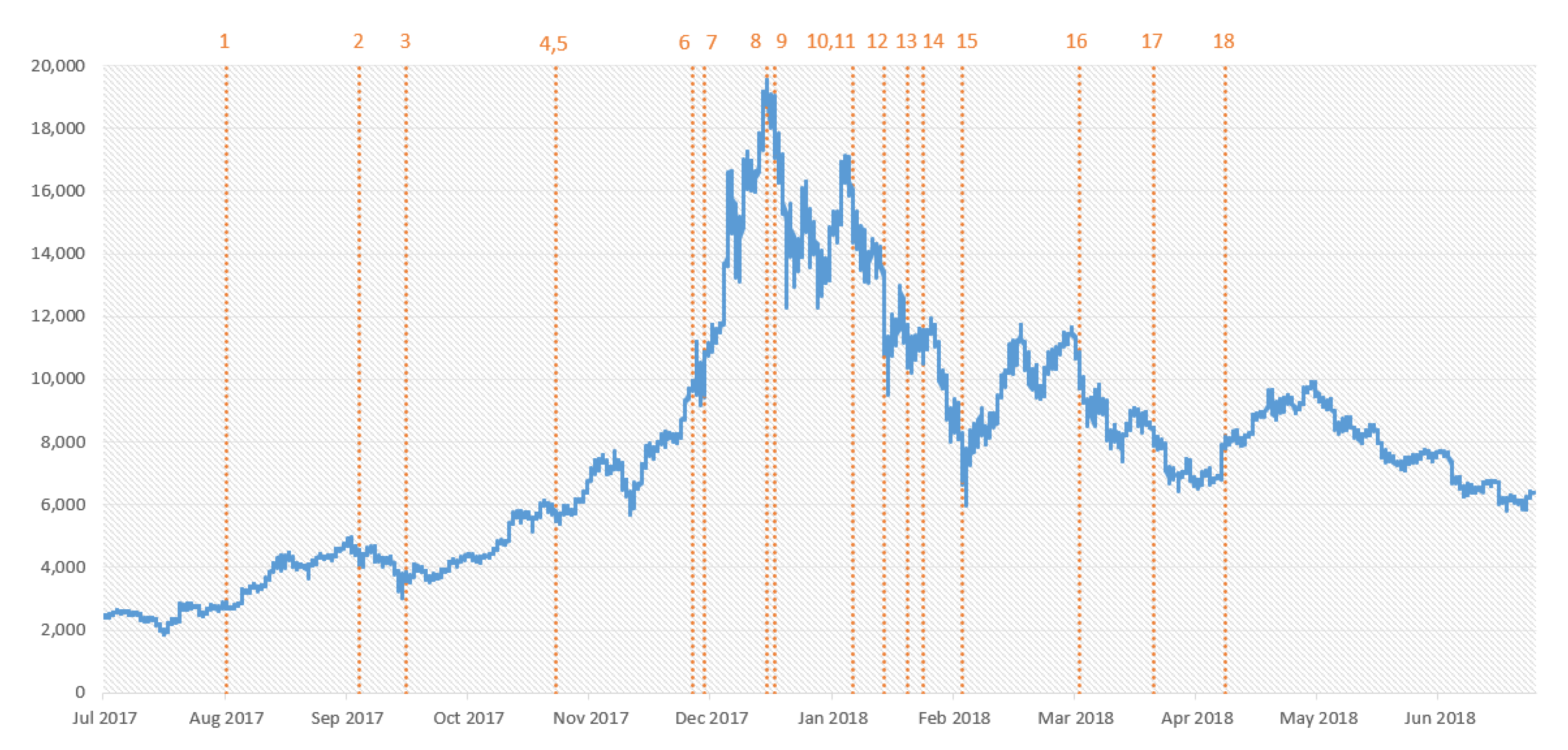
Our empirical analysis examines the most widely known and capitalized cryptocurrency in current times: Bitcoin. We considered hourly Bitcoin exchange prices expressed in USD sampled on hourly basis. We analyzed a one year time-frame which ranges from 1 July 2017 to 30 June 2018, counting 8750 observations1. The timespan analyzed includes two sub-periods of great interest for crypto investors: the spectacular price growth in 2017 and its correction in 2018. The period was chosen to be quasi-symmetric around bull and bear times.

During the two sub-periods, many events involving cryptocurrencies occurred and some of them have meaningfully affected their price dynamics, mostly Bitcoin. The main events are summarized in

Table 1. Main events related to cryptocurrencies.

Date	Event	Description
(1) 01/08/2017	Bitcoin Cash hard fork	Bitcoin forked into two derivative digital currencies, the Bitcoin (BTC) chain with 1 MB blocksize limit and the Bitcoin Cash (BCH) chain with 8 MB blocksize limit.
(2) 04/09/2017	China banning Initial Coin Offerings (ICOs)	People’s Bank of China banned fund raising by ICOs referring to the threat to economic and financial stability. Largely due to the high amount of suspicious ICOs accused of illegally raising money and aiding intentional fraud.
(3) 16/09/2017	China exiting local trading	Chinese authorities announced a ban on trading cryptocurrencies at national exchange services. Firstly, leaked documents were online just four days after the ban of ICOs, on 8 September. On 15 September the Chinese platforms Huobi and OKCoin announced that they will halt trading for local customers by 31 October.
(4) 24/10/2017	Japan establish a self-regulatory industry body	The Financial Services Agency (FSA), the responsible overseer of banking, securities, insurance, and exchange sector of Japan, set up the Japan Virtual Currency Exchange Association (JVCEA)—a consortium of 16 FSA-approved domestic cryptocurrency exchanges—to establish as a certified fund settlement business association.
(5) 24/10/2017	Coinbase received New York state banking license	Coinbase Custody received a license to operate as an independent qualified custodian, i.e., a Limited Purpose Trust Company chartered by the New York Department of Financial Services (NYDFS).
(6) 28/11/2017	Bitcoin price $ 10,000	Bitcoin price reaches the level of $10,000.
(7) 01/12/2017	CFTC Bitcoin futures approval	The Commodities Futures Trading Commission (CFTC) approved the request by CME Group and Cboe Global Markets to launch Bitcoin futures. The two markets, which were launched on December 10 and 18, respectively, allow investors to bet on the future price of Bitcoin.
(8) 17/12/2017	Bitcoin price $20,000	Bitcoin price reaches the level of $20,000.
(9) 19/12/2017	Yapian filed for bankruptcy	Yapian, a company owning the Youbit cryptocurrency exchange in South Korea, filed for bankruptcy following a hack, saying it lost 17% of its assets.
(10) 08/01/2018	China scrutinizing mining	The Public Bank of China started to investigate Bitcoin mining and outlined the plan to deter Bitcoin miners by limiting power consumption.
(11) 08/01/2018	Korean crypto bank accounts investigation	Korean financial authorities launched an investigation into cryptocurrency-related services provided by local banks. In particular, the Financial Intelligence Unit (FIU)—a body under the Financial Services Commission (FSC) which monitors illegal financial activities—and the Financial Supervisory Commission - the country’s financial supervisor—were looking into cryptocurrency-related virtual accounts at six local banks to check their compliance with anti-money laundering regulations.
(12) 16/01/2018	Bitconnect exchange shut-down announcement	Bitconnect announced it would shut down its cryptocurrency exchange and lending operation after North Carolina and Texas regulators issued a cease-and-desist order against it, stating it was suspected of being fraudulent.
(13) 22/01/2018	South Korean regulation about anonymity	South Korea brought in a regulation requiring all Bitcoin traders to reveal their identity, hence banning anonymous trading of Bitcoins.
(14) 26/01/2018	Coincheck hacked	Japan’s largest cryptocurrency OTC market, Coincheck, was hacked and as much as 530 million USD of NEMs were stolen, causing Coincheck to suspend trading.
(15) 05/02/2018	China’s announcement of blocking foreign trading	With the aim of preventing Chinese investors from financial risks, as in September 2017, China’s authorities announced their willingness to ban trading of cryptocurrencies by blocking internet access to foreign trading platforms.
(16) 07/03/2018	Irregular trades	Compromised Binance API keys were used to place irregular trades.
(17) Late 03/2018	Social network bans	Facebook, Google, and Twitter banned advertisements for ICOs and token sales.
(18) 13/04/2018	Coinsecure robbery	Coinsecure, one of India’s biggest exchange platforms, lost 438 Bitcoins as a result of a theft. Based on the prices at the time of the occurrence of the event this translates to approximately 3 million $ (i.e., roughly 190 million rupees in local currency).

Note: The table reports major events related to cryptocurrencies during the sample period analyzed in the paper, i.e., 1 July 2019–30 June 2019.

. Some notable events include: In the beginning of September 2017, People’s Bank of China ban of fund raising by Initial Coin Offerings (ICOs) was linked this with a 5 % drop in the Bitcoin price. This was followed by the dramatic announcement by the Chinese authority to shut down trading of cryptocurrencies at national level. In early December, the approval of Bitcoin futures by the Commodities Futures Trading Commission (CFTC) had a high impact on Bitcoin investors. Bitcoin price spectacularly grew from around 10,000 USD a coin when the news broke to a high just below 20,000 USD on 18 December; at the beginning of 2018, the South Korean regulators banned anonymous bank accounts being used to buy and sell cryptocurrencies. After that move, Bitcoin price declined from just below 11,000 USD to a daily low of 10,179 USD. The Bitcoin price fall then continued and was accompanied by many negative news regarding cryptocurrencies. Indeed, during the first half of 2018, the exchange platform Bitconnect shut down, Coincheck was hacked and Coinsecure was robbed, leading to unavoidable price declines. Moreover, the Bitcoin price suffered from the moves of the Chinese government towards blocking all websites that enable cryptocurrency trading and ICOs and foreign platforms that enable Bitcoin trading in February, as well as from the social network bans on advertisements for ICOs and token sales.

We studied return connectedness of five major Bitcoin market exchanges, meaning Bitstamp, Gemini, Coinbase, Kraken, and Bittrex2. The main features of the Bitcoin exchange platforms analyzed in this study are summarized in

Table 2. Bitcoin exchange features.

	Bitstamp	Gemini	Coinbase	Kraken	Bittrex
Launched	Jul 2011	Oct 2014	May 2014	Jul 2011	Feb 2014
Headquarter location	UK	USA	USA	USA	USA
Trading pairs	14	15	53	95	355
BTC trading volume during analyzed period	6.37 M	2.63 M	7.46 M	5.46 M	NA
Trading fees	0.10–0.25%	0.00–0.25%	0.10–0.30%	0.00–0.25%	0.25%
Fiat currencies withrawal/deposit time	1–5 business days	4–5 business days	1–5 business days	1–5 business days	-
Supported currencies	USD, EUR	USD	USD, EUR, GBP	CAD, EUR, GBP, JPY, USD	USDT

Note: The table summarizes the characteristics of the Bitcoin exchanges investigated in the study at the date of 05/10/2019. Maker fees may be smaller than taker fees and fees may be lower for high trading sizes.

. Bitstamp and Kraken are two of the oldest cryptocurrency exchanges existing, whereas Gemini, Coinbase, and Bittrex are relatively newer ones. Except for Bitstamp, whose headquarter is located in the UK, all the exchanges included in the sample are U.S.-based. The number of traded pairs varies quite a lot across exchanges, with Bitstamp and Gemini being the ones trading the smallest number coin pairs and Bittrex the one showing more variety of trading pairs. Trading fees are generally quite comparable across the analyzed exchanges, whereas trading volumes during the analyzed time-frame are all above 5 million USD, and the time to withdraw or deposit fiat currencies is generally between 1–5 business days, except for Gemini, which shows lower trading volumes and higher withdrawal and deposit time of fiat currencies. As far as the supported currencies, Kraken is the one supporting the biggest number of fiat currencies, whereas Gemini and Bittrex support only USD and USDT, respectively.

Given that in our analysis we consider the price of the same crypto (Bitcoin) traded on different venues, prices exhibit almost identical dynamics—i.e., they co-move. Therefore, without loss of generality, we plot the Bitstamp price series during the considered period in Figure 1, highlighting the main events related to cryptocurrencies described in Table 1.

A simple visual inspection yields to the conclusion that the upward and downward trend periods split the sample into two almost equal time-frames. More importantly, from an econometric point of view, it can be noticed that the Bitcoin price series seem to be highly non-stationary in levels, arguably $I\left(1\right)$. This consideration, together with the non-deviation of Bitcoin exchange prices in the long run prescribed by the law of one price, made us expect a cointegrating relationship among the Bitcoin price series we analyzed.

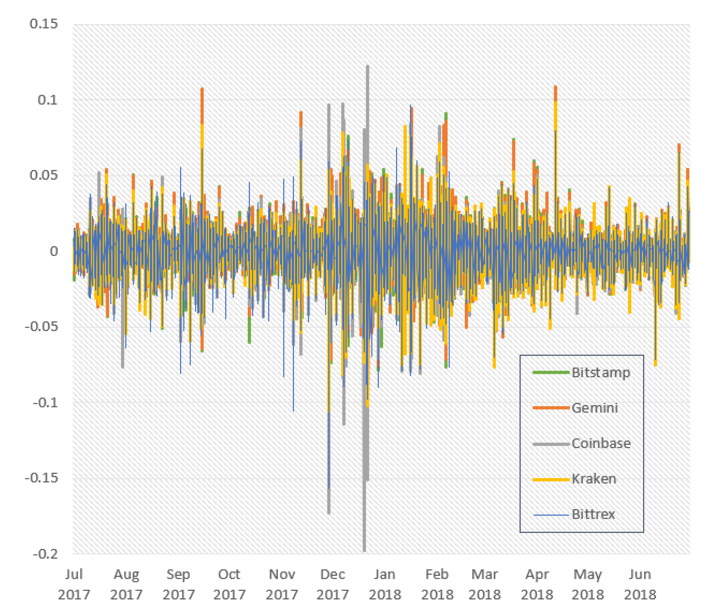
For the sake of completeness, we also plotted the continuous returns of the exchange price series in Figure 2.

In this case, we noticed a few data points in which there is a consistent disequilibrium in returns, meaning that they diverge quite drastically. This suggests that some exchanges behave dissimilarly to others during certain periods. The latter proposition is also supported by the summary statistics contained in

Table 3. Summary Statistics of Returns.

	Bitstamp	Gemini	Coinbase	Kraken	Bittrex
Mean	0.0001	0.0001	0.0001	0.0001	0.0001
Median	0.0002	0.0001	0.0009	0.0006	0.0006
Maximum	0.1079	0.1083	0.1220	0.0980	0.0969
Minimum	−0.1076	−0.1222	−0.1979	−0.1052	−0.1565
Std. Dev.	0.0122	0.0121	0.0122	0.0115	0.0124
Skewness	0.0497	0.1303	−1.3244	−0.5429	−0.9601
Kurtosis	8.0090	9.3869	25.3352	9.4711	11.2719

Note: The table includes relevant summary statistics for returns related to the analyzed exchanges considering the entire sample period.

. Again, from an econometric point of view, the graph showing continuous returns provides evidence to the hypothesis that Bitcoin price series are $I\left(1\right)$ time series, which will be empirically tested in the following.

As a preliminary analysis, we need to ensure that the analyzed time series are characterized by a non-stationary and cointegrated behavior. To this aim, we conducted two widely employed stationarity and cointegration tests.

To test for (non-)stationarity, we performed the Augmented Dickey–Fuller (ADF) tests—see Dickey and Fuller (1979)—on prices, expressed in log-levels. The test results are shown in

Table 4. Augmented Dickey–Fuller test.

	Bitstamp	Gemini	Coinbase	Kraken	Bittrex
p-value${}_{log-levels}$	0.7669	0.7718	0.7232	0.7945	0.7440
p-value${}_{log-returns}$	<0.0100	<0.0100	<0.0100	<0.0100	<0.0100

Note: The table shows the resulting p-values for the Augmented Dickey–Fuller (ADF) test considering the entire sample period. The test in levels includes a constant but no time trend in the model specification. The minimum p-value reported is 0.01.

.

The ADF test provides strong support towards the non-stationarity of the price series in log-levels, whereas it provides evidence for stationarity of their first differences—i.e., of continuous returns. This is true for all conventional significance level. Therefore, we can claim that the Bitcoin price series analyzed are $I\left(1\right)$ time series.

To test for cointegration, we employed the Johansen trace test, as proposed by Johansen (1991). In line with our methodological approach, we expected to find a cointegrating rank of the system which amounts to $h=n-g=5-1=4$. This is because the law of one price entails that prices related to the same asset should be driven by $g=1$ unique common stochastic trend. The test outcomes are illustrated in

Table 5. Cointegration (Johansen Trace test).

	Test Stat	Critical 10%	Critical 5%	Critical 1%
h <= 4	3.10	6.50	8.18	11.65
h <= 3	188.84	15.66	17.95	3.52
h <= 2	752.42	28.71	31.52	37.22
h <= 1	1627.95	45.23	48.28	55.43
h = 0	3230.01	66.49	70.60	78.87

Note: The table illustrates the test statistics statistics and critical values for the Johansen Trace test for cointegration for the full sample period. The test does not include any costant nor time trend, neither in the model specification nor in the cointegrating relationship.

.

The test statistics allow us to reject the null hypothesis of a cointegrating rank h of at most 3 against the alternative of a cointegrating rank of 4. In other words, the test suggests a cointegrating rank of the system $h=4$, i.e., the presence of $g=1$ common stochastic trend driving the fundamental Bitcoin price, in line with our previous considerations. This guarantees assumptions are met and the methodology can be soundly applied to our real data.

5. Empirical Findings

In this paper, we investigated Bitcoin exchange return connectedness from a dynamic viewpoint. In other words, rather than estimating spillover measures on the full sample period, which would provide the “average” or “unconditional” connectedness, we estimated spillover indexes on rolling windows, with the aim to explore the dynamic features of exchange interconnectedness. In particular, we set a predictive horizon for the variance decomposition of $H=12$. As far as the approximating model is concerned, we used a VECM lag length of 2, corresponding to a lag length of 3 in its vector autoregressive representation. We then considered a one-sided estimation rolling window of $w=336$ h—corresponding to two weeks3.

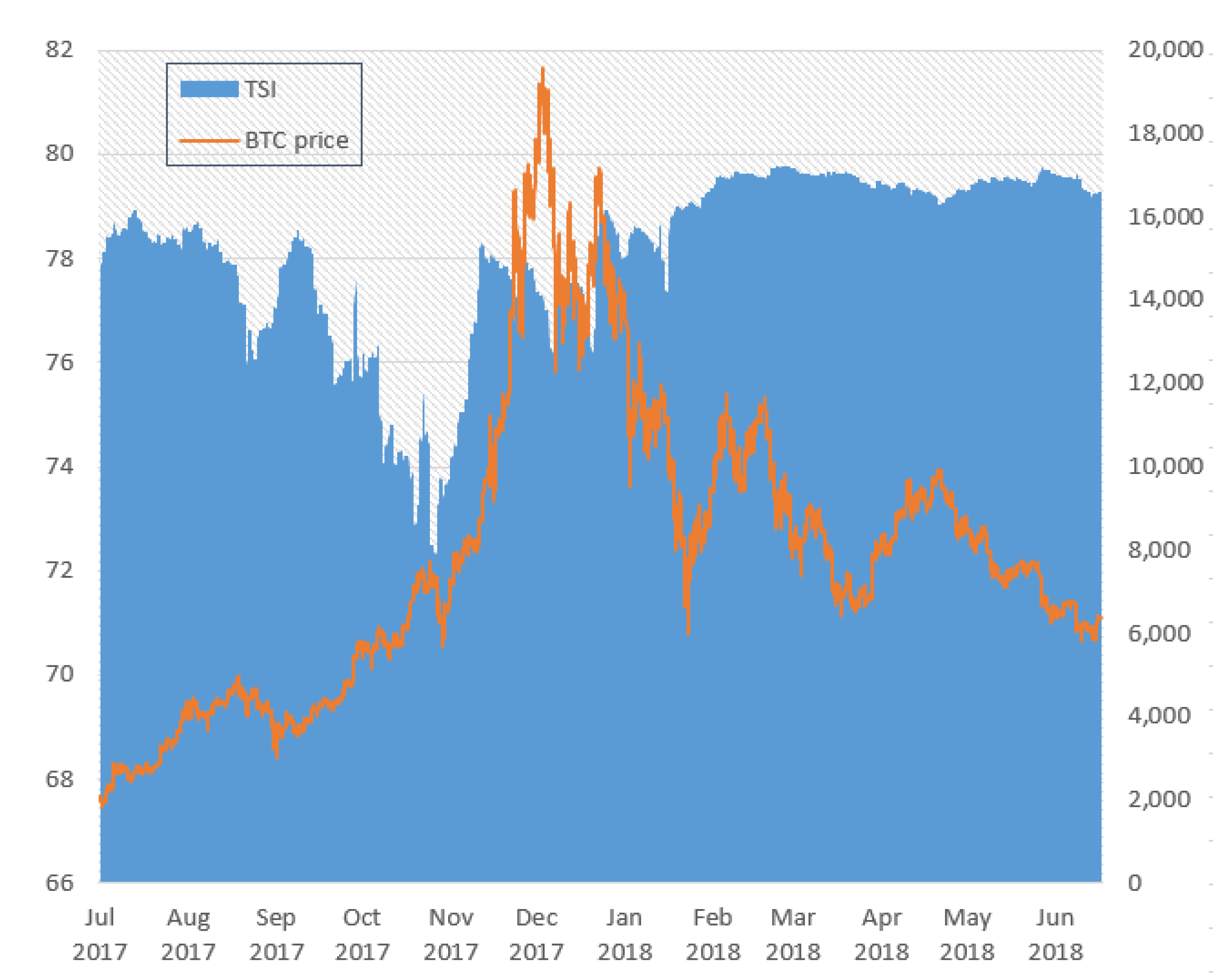
Firstly, we derived the total return spillover index and provided its plot—together with the Bitstamp Bitcoin price related to the same period—in Figure 3.

The total return spillover index ranges from a minimum of 72.24% to a maximum of 79.79%, with an average value of 78.13% over the examined period. This suggests that system-wide return connectedness is relatively high when considering Bitcoin exchanges.

Similarly to the Bitcoin price, the TSI seem to show two main cycles: one in which the index witness a downward trend, as well as a following one where it steadily grows and finally smooths out. However, its dynamics are not synchronized with that of the Bitcoin price. This suggests that both in hype and correction periods interconnectedness may either lower or increase depending on specific market features.

In our case, system-wide connectedness generally fell during the first cycle, specifically until the beginning of November 2017 period, in which the Bitcoin price started an unprecedented year-end rally. Right after the minimum peak of the index, Bitcoin prices began to surge like never before, and the index goes back rapidly to its previous values. This means that, while during the first price growth phase we encountered interconnectedness among Bitcoin exchanges lowers, contagion effects begin to be more consistent during the year-end Bitcoin price hype. During the second cycle, the TSI wiggles and grows at first, whereas it levels out and stabilizes in the range 79–80% starting from February 2018. This also coincides with the end of the hard correction of Bitcoin price, after which exchange interconnectedness becomes relatively steady.

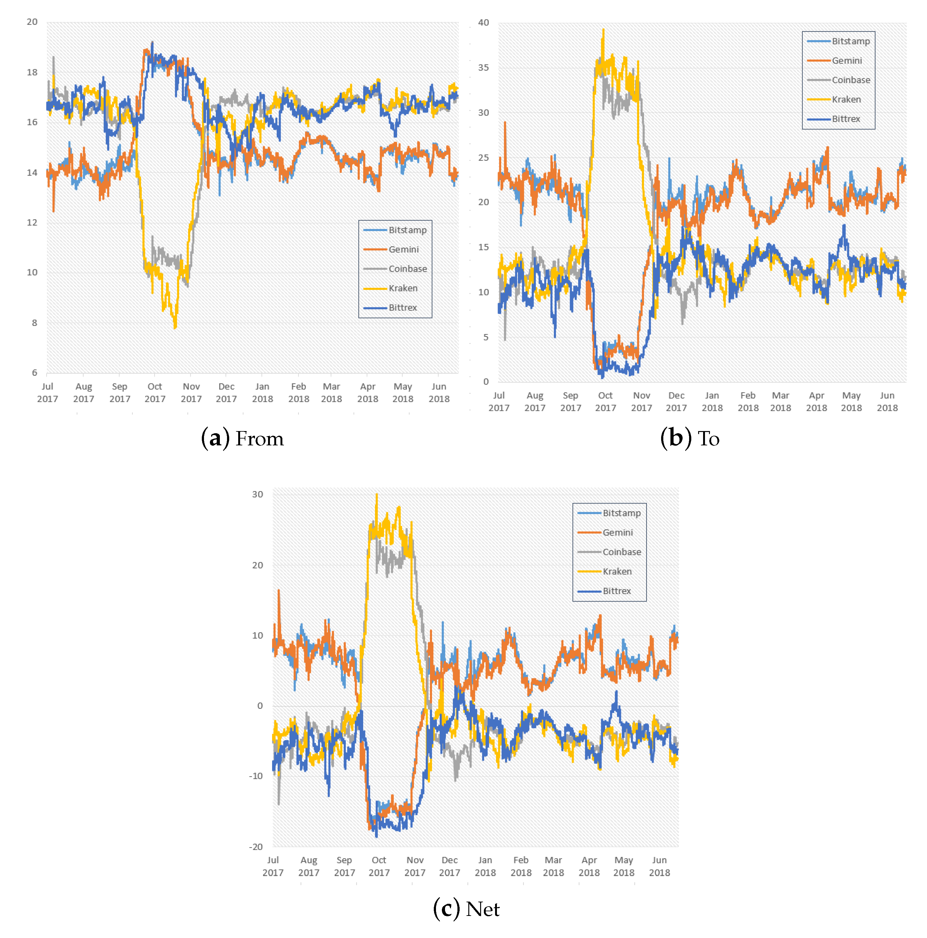
After that, we studied the directional return spillover indexes, i.e., the “from”, “to”, and “net” spillover indexes. A plot illustrating their dynamics over the considered time-frame is contained in Figure 4.

At first glance, one may notice that the range of variation related to the directional spillovers to others is wider than that of the directional spillovers from others. Indeed, while the return spillover indexes from others range from a minimum of 7.80% to a maximum of 19.23%, the spillovers indexes to others show a minimum of 0.47%, a maximum of 39.32% during the studied period. This reflects into an as wide range for the net return spillover indexes, with values between −18.57% and 30.13%.

In general, we find that to some extent there is a kind of equilibrium with regards to the directional spillovers from and to others, as well as in the net ones. During most of the analyzed period, Bitcoin exchanges can be split into two groups: those who transmit return spillovers to others, namely Bitstamp and Gemini, and those who instead receive return spillovers, i.e., Bittrex, Coinbase, and Kraken. This can be immediately stated by a visual inspection of the net spillover indexes in Figure 4, which give us a hint on the leading and following Bitcoin exchanges during the analyzed time-frame. Moreover, we may add that the dynamics and magnitude of the directional return spillovers is quite similar within the same group.

However, there is a specific period in which the equilibrium witnesses a substantial instability. This is related to the same period in which the total return spillover index starts to rise after a steady decline. The directional spillover indexes suggest that in this phase Kraken and Coinbase rapidly start transmitting return spillovers to others, and they keep doing that until the dramatic year-end price surge, whereas Bitstamp and Gemini receive spillovers during the same phase, together with Bittrex. The strong change in leadership pushes from 20% to 5% the transmitted spillover contributions of the two exchanges leading before in less than one month, besides making that of Bittrex drop to almost null values.

The unique exchange which constantly emerges as a return spillover receiver—even more in the latter mentioned timespan—is Bittrex, being its net spillover index values as much as 96.98% of the times below 0. This is in line with the fact that leading exchanges are generally those in which most of the trading volumes lie, as Bittrex is the smallest exchange we selected in terms of trading volumes.

After the year-end Bitcoin price surge, directional spillover indexes go back to their previous equilibrium. Indeed, the down market not only brings system-wide connectedness to its previous levels but also re-establishes the exchange ranking in terms of return shock transmitted. In particular, despite some fluctuations from the end of 2017 onwards, Bitstamp and Gemini re-confirmed their previous leading position, while Bittrex, Kraken, and Coinbase were that of follower.

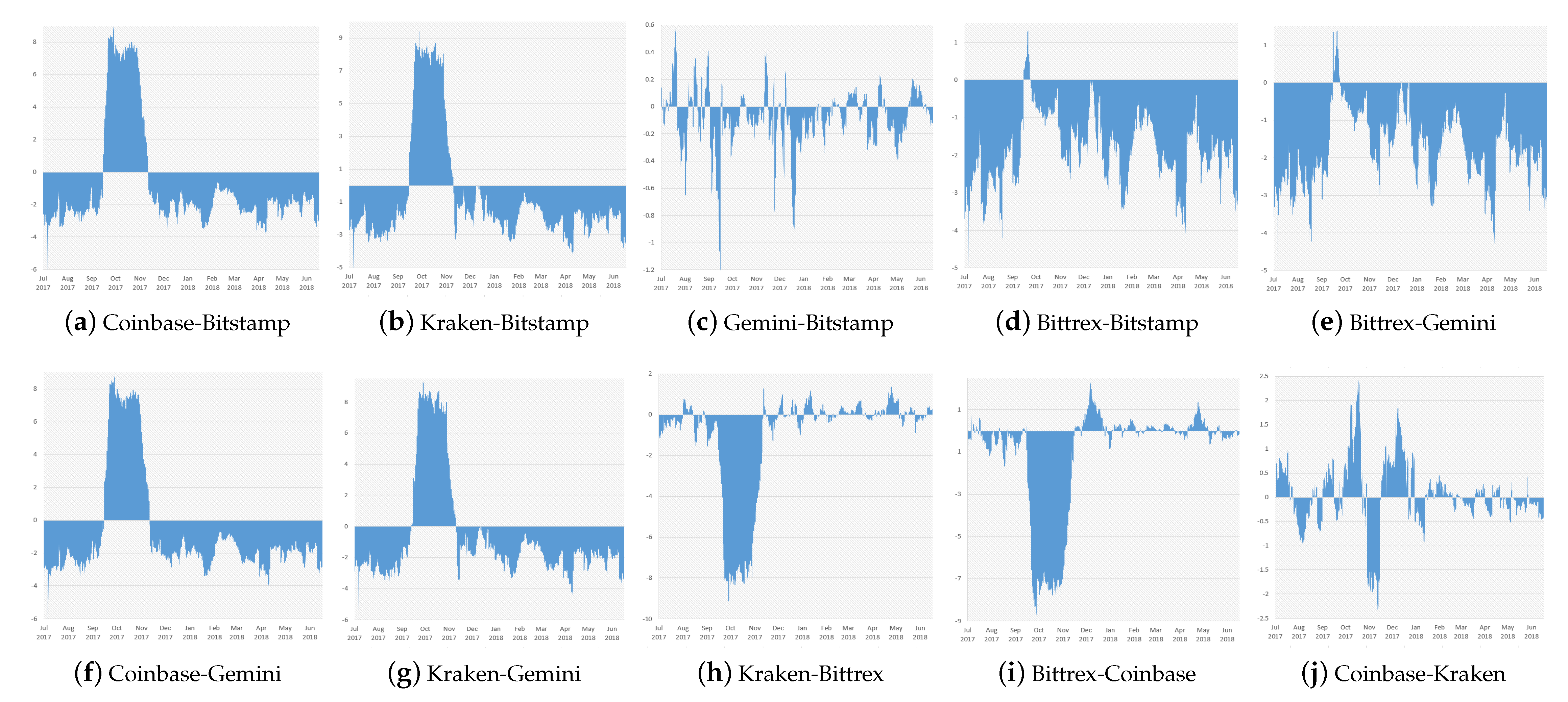
Finally, we explored the net pairwise spillover indexes, which give us information on how return shocks are transmitted across Bitcoin market exchanges, from a pairwise viewpoint. We plotted the net pairwise spillover indexes in Figure 5.

First of all, pairwise spillover indexes vary in wide ranges, meaning that pairwise connectedness relationships show considerably different magnitudes across exchange pairs. To illustrate, the narrowest range of variation can be found in the pairwise spillover index between Gemini and Bitstamp, which shows a minimum of −3.56 and a maximum of 1.07, whereas the widest range in the index is that of Bitstamp and Coinbase, that is from −6.19% to 8.88%—more than three times the latter one.

The study of net pairwise spillover indexes provides more depth to the conclusions on the exchange interconnectedness that emerged from the total and directional spillover indexes analysis. Overall, Bitstamp and Gemini transmit a significant portion of return spillovers to all other exchanges, with Bittrex being the most affected. However, in line with the earlier findings, during the period before the year-end price hype, Coinbase and Kraken transmit shocks to all other exchanges, with relatively high and comparable magnitudes.

It is interesting to study the interaction between the exchanges on the top of the ranking. The net pairwise spillover index between Gemini and Bitstamp oscillates around the zero line and assumes relatively low values. From a visual inspection, Bitstamp seems to dominate Gemini in terms of return spillover transmission, both in terms of timespan and magnitude. As a matter of fact, the net pairwise spillover index Gemini-Bitstamp assumes negative values as much as almost two-thirds (66.58%) of the time. Moreover, the contribution of Gemini towards Bitstamp does rarely overcome a value of 0.4, as opposed to the return spillovers transmitted from Bitstamp to Gemini, which not only double but even triple in size.

For the sake of ranking completeness, we also investigated the relationship between Coinbase and Kraken. It is not clear from a graphical point of view which exchange contributes more in terms of return spillover. Contribution magnitudes show quite comparable ranges, and the number of times Coinbase transmits shocks to Kraken is almost the same as the opposite situation (49.01%). It is clear that the two exchanges interact in a different way with respect to the two leading ones, as their net pairwise spillover index oscillates much less around 0. This means their role of transmitter and receiver are more stable over time than in the previous case.

To summarize our empirical contribution in a nutshell, we are able to shed further light on price discovery among Bitcoin exchange markets. Previous papers, such as (Brandvold et al. 2015; Pagnottoni and Dimpfl 2018; Giudici and Pagnottoni 2019), found that the exchange markets with higher traded volumes are typically the ones that drive prices and spillovers. Differently from the previous papers, based on daily price data, we considered high frequency data. The analysis of this data led to confirm the conclusions from the previous papers. In addition, it allowed an important discovery on the dynamic nature of return spillovers: Although stable to some extent, the lead-lag relationship among Bitcoin exchanges is dynamic and witnesses notable changes over time. These changes may be fundamental for both policymakers and investors, who should monitor them for the purpose of an efficient decision-making process and investment decision, respectively.

6. Robustness

In this section, we propose a robustness analysis of our results with respect to the choices of the parameters used in the modeling strategy. To illustrate, we examine the total return spillover index for alternative rolling windows w set for the model estimations and alternative predictive horizons H. We increased and decreased the window width and predictive horizon by +50% and −50%, resulting in window width choices of $w=168,336,504$ and predictive horizon choices of $H=6,12,18$.4 In this way, we investigate the robustness of the TSI when considering rolling estimation windows of 1, 2, and 3 weeks, as well as predictive horizons of $\frac{1}{4}$, $\frac{1}{2}$, and $\frac{3}{4}$ of a day. Plots related to the alternative total spillover in TSI are shown in Figure 6.

The TSI seems to be just slightly influenced by changes in the window width w. As one may expect, the larger the rolling window the smoother is the index, whereas tighter windows yield to a more fluctuating one. However, in our case, we can state that results are qualitatively unaffected by the choice of the rolling window.

The index appears to be more sensitive to the choice of the forecast horizon H to compute the forecast error variance decompositions rather than to the rolling window. However, there is much more similarity in the behavior of the spillover index between choices of the forecast horizons H of 12 and 18 rather than those of 6 and 12. This suggests that a judicious predictive horizon choice should grant stability of the index without losing information about its surge or decline and related magnitude. More importantly, the dynamics of the indexes show quite similar patterns, which just differ in their scale of values. This means that—once more—the qualitative interpretation of our results is not influenced by the choice of the predictive horizon H.

To conclude, our empirical outcomes appear robust with respect to the rolling window set for the estimation and the predictive horizons used in the forecast error variance decompositions.

7. Conclusions

This paper explores system-wide and directional connectedness, along with price discovery mechanisms among five major Bitcoin exchange markets. This is done by extending the Diebold and Yilmaz (2012) forecast error variance decomposition from a VAR to a VECM framework, which enables us to take into account the non-stationary and cointegrated behavior of the time series analyzed.

We remark that the methodological improve illustrated above is neither exclusively tied to Bitcoin exchange platforms nor to cryptocurrency ones. Indeed, this technique can be extended to the study of interconnectedness among all exchange platforms trading the same financial products.

Our results show that overall connectedness strongly evolves over time and, in particular, it generally decreases during bull market times and decreases during down market periods. We also find that Bitfinex and Gemini can be all over considered as leading exchanges in the price formation process, being mostly a transmitter of a significant portion of return spillover during the considered timespan. On the other hand, we identify Bittrex as follower, given it acts as a receiver of return shocks during the whole time period considered.

We also highlight the dynamic nature of return spillover across Bitcoin exchanges, as they considerably evolve over time. This means that the lead-lag relationships existing among Bitcoin exchanges is not constant and is subject to changes over time.

From a practical viewpoint, our results suggest that, to predict the direction of price movements and contagion effects, potential investors should pay attention to spillovers and, particularly, to the exchanges that have the highest trading volumes, in general. However, the time dynamics should also be taken into account, with a particular eye on events that may affect price volatilities and spillovers. This is also true for policymakers, who can come up with more efficient decision-making by monitoring spillover effects due to events belonging to the regulatory framework.

Future research may include different model paradigms, based on Bayesian analysis—as in (Giudici et al. 2003; Figini and Giudici 2011), on network models—as in Giudici and Bilotta (2004)—or on extreme value models—as in Calabrese and Giudici (2015).