Credit Valuation Adjustment Compression by Genetic Optimization

Abstract
1. Introduction
Outline and Contributions
2. CVA Compression Modeling
2.1. Credit Valuation Adjustment
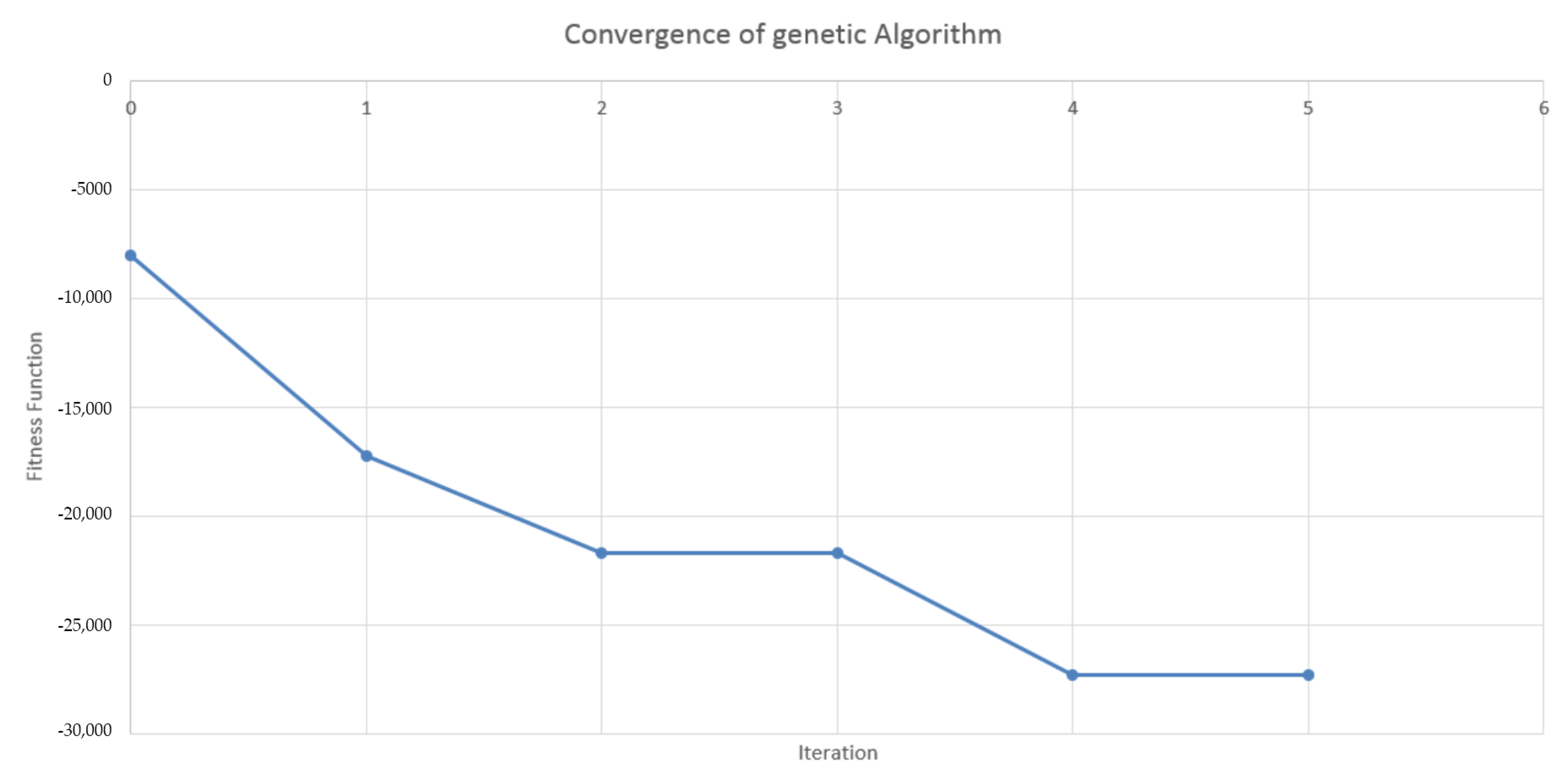
2.2. Fitness Criterion
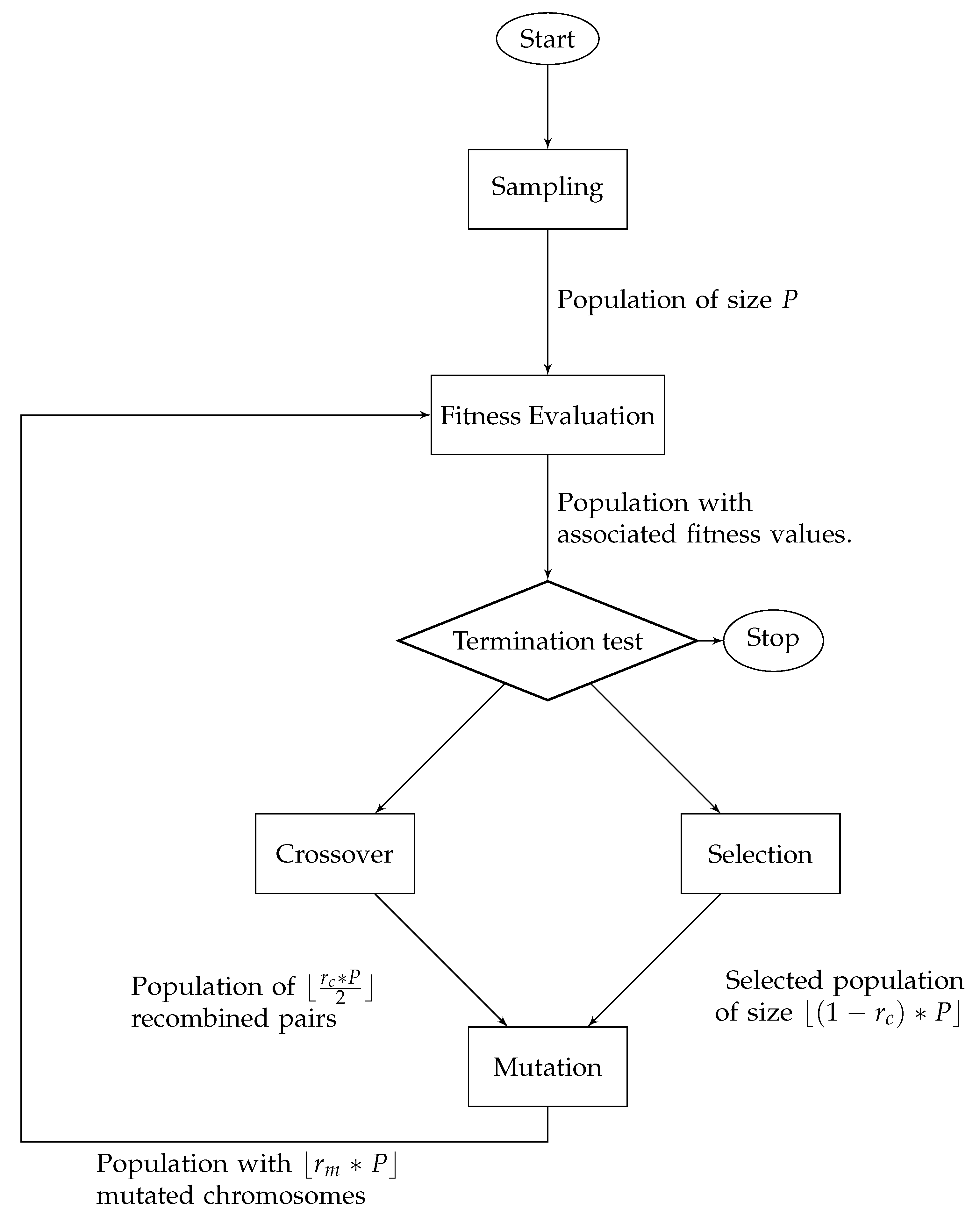
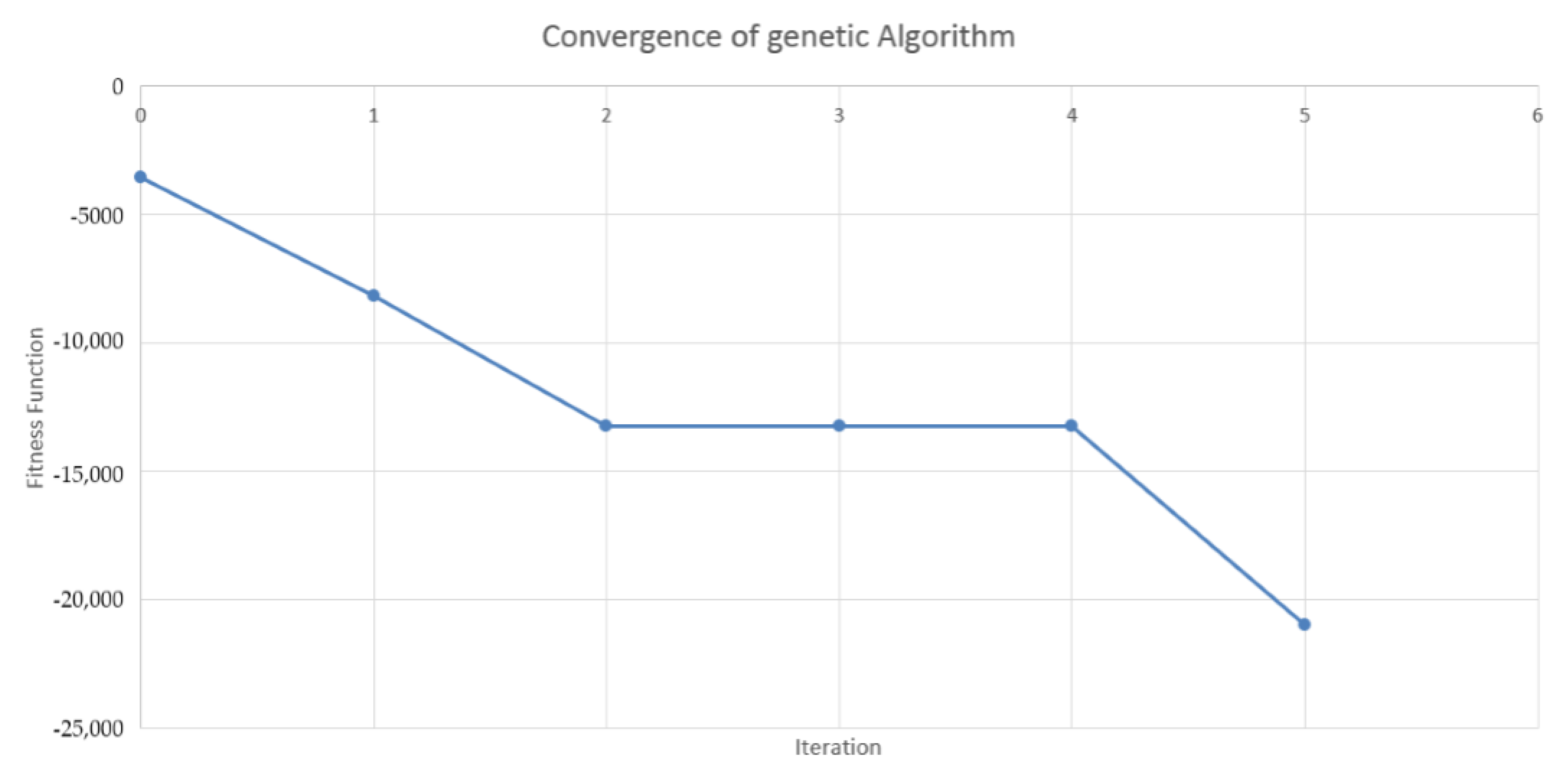
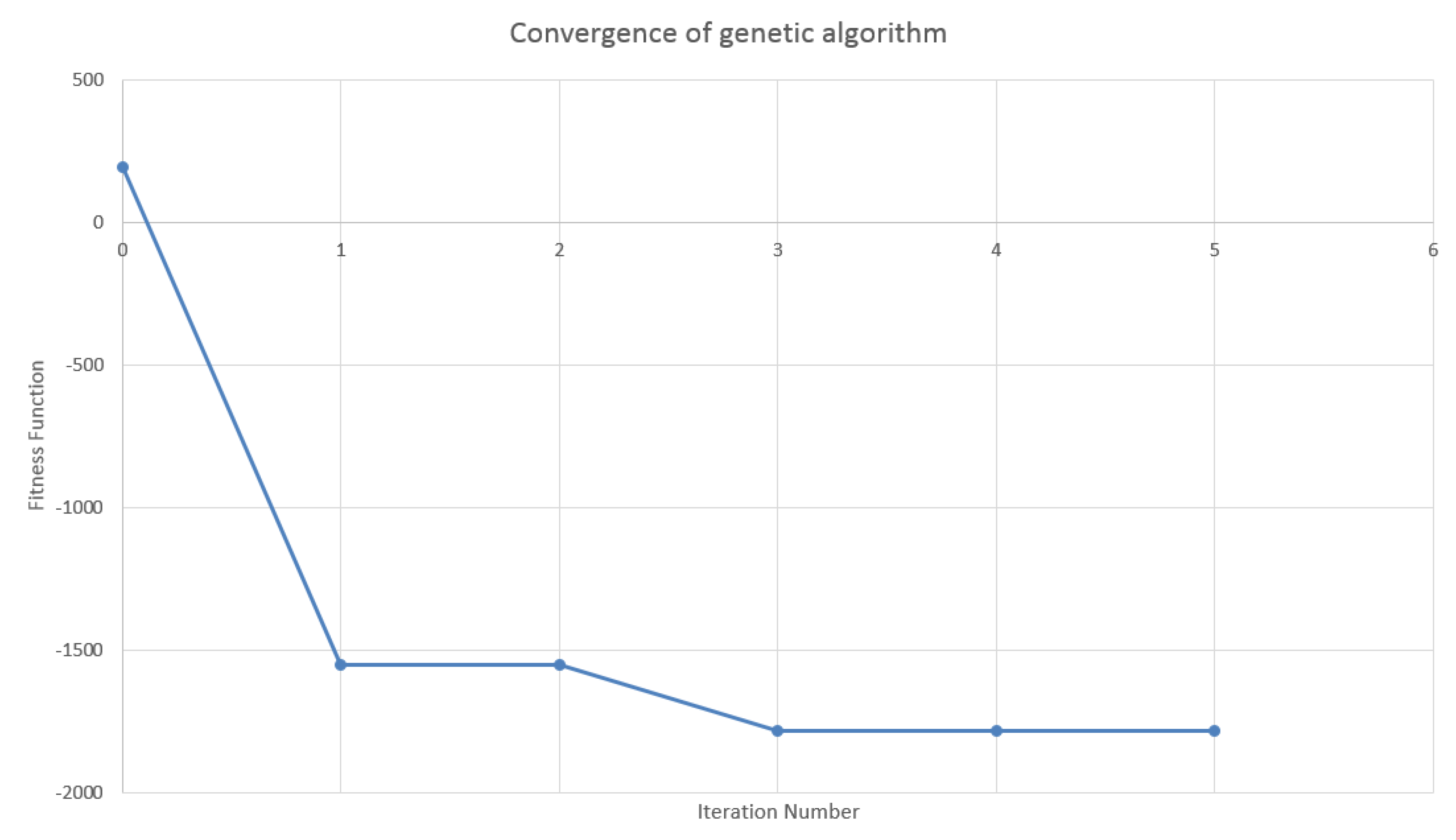
2.3. Genetic Optimization Algorithm
| Algorithm 1: Pseudo-code of an optimization genetic algorithm |
 |
3. Acceleration Techniques
- a MtM store-and-reuse approach for trade incremental XVA computations, speeding up the unitary evaluation of the fitness function; and
- a parallelization of the genetic algorithm accelerating the fitness evaluation at the level of the population.
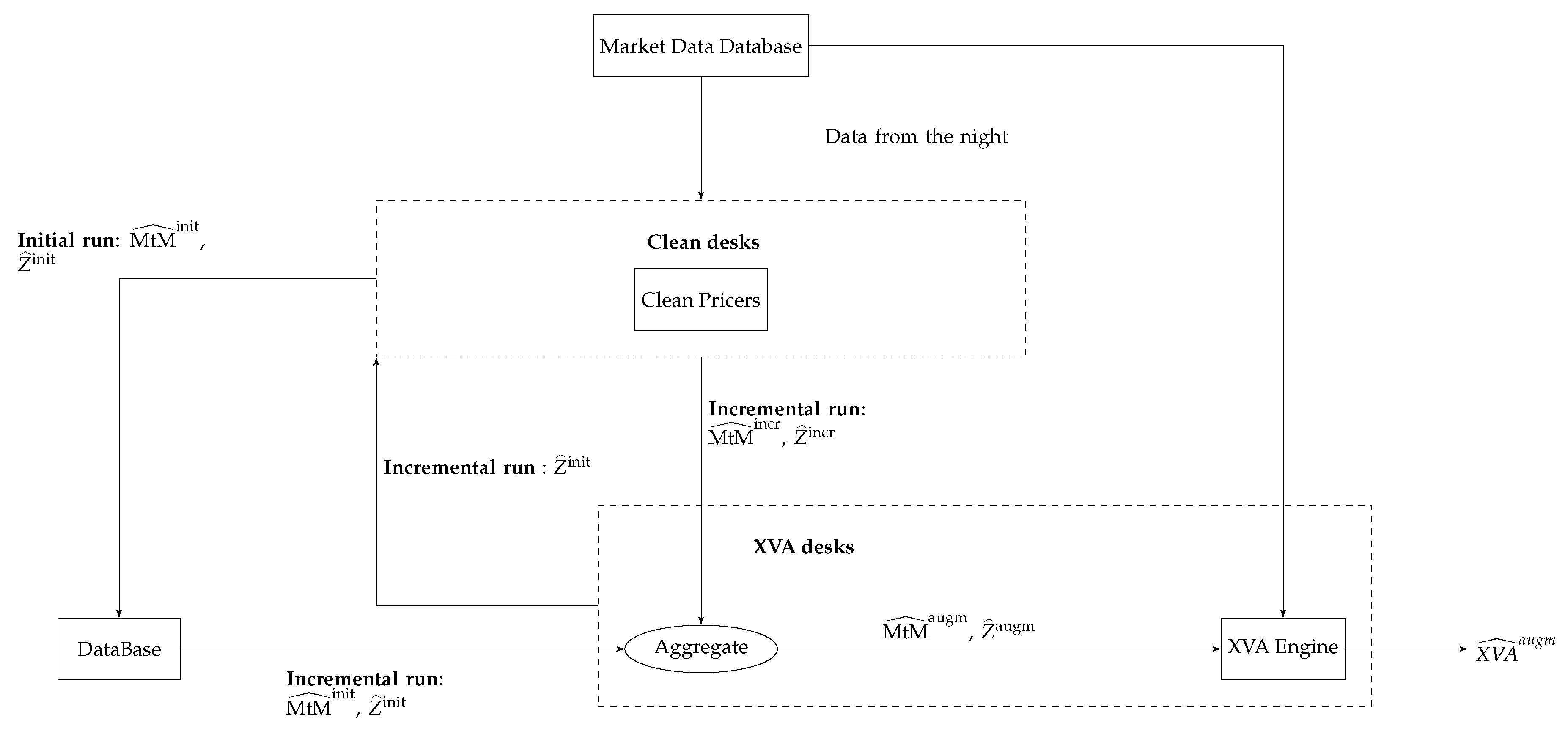
3.1. MtM Store-and-Reuse Approach for Trade Incremental XVA Computations
- (No nested resimulation of the portfolio exposure required) The formula for the corresponding (portfolio-wide, time-0) XVA metric should be estimatable without nested resimulation, only based on the portfolio exposure rooted at . A priori, additional simulation level makes impractical the MtM store-and-reuse idea of swapping execution time against storage.
- (Common random numbers) should be based on the same paths of the drivers as . Otherwise, numerical noise (or variance) would arise during aggregation.
- (Lagged market data) should be based on the same time, say 0, and initial condition (including, modulo calibration, market data), as . This condition ensures a consistent aggregation of and into .
- The first seems to ban second-order generation XVAs, such as CVA in presence of initial margin, but these can in fact be included with the help of appropriate regression techniques.
- The second implies storing the driver paths that were simulated for the purpose of obtaining ; it also puts a bound on the accuracy of the estimation of , since the number of Monte Carlo paths is imposed by the initial run. Furthermore, the XVA desks may want to account for some wrong way risk dependency between the portfolio exposure and counterparty credit risk (see Section 2.1); approaches based on correlating the default intensity and the market exposure in Equation (5) are readily doable in the present framework, provided the trajectories of the drivers and/or risk factors are shared between the clean and XVA desks.
- The third induces a lag between the market data (of the preceding night) that are used in the computation of and the exact process; when the lag on market data becomes unacceptably high (because of time flow and/or volatility on the market), a full reevaluation of the portfolio exposure is required.
3.2. Parallelization of the Genetic Algorithm
4. Case Study
- Which type of swap is suitable for achieving the compression of the CVA, in the context of a given initial portfolio?
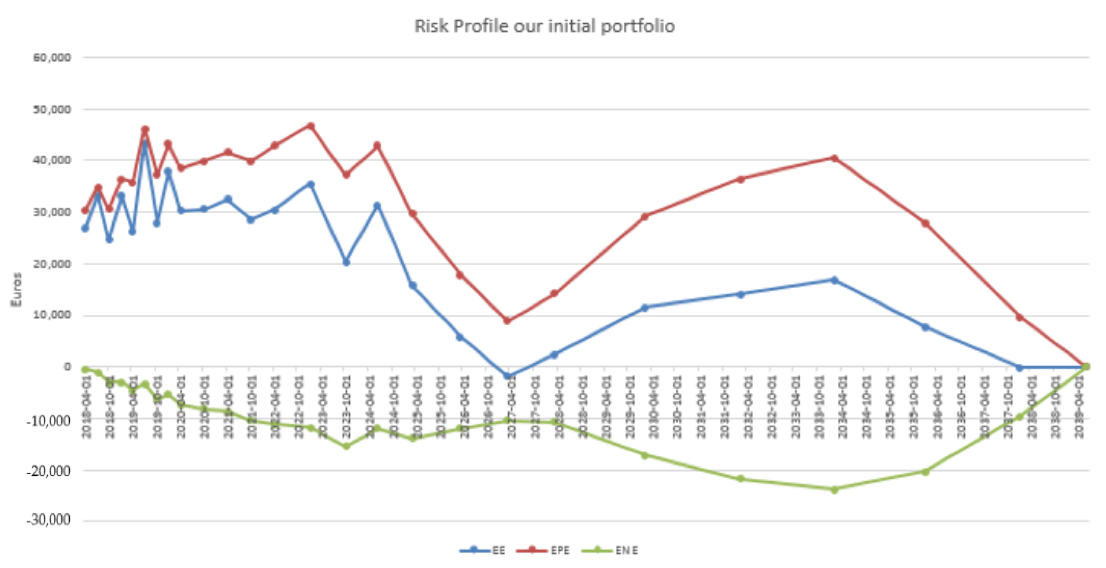
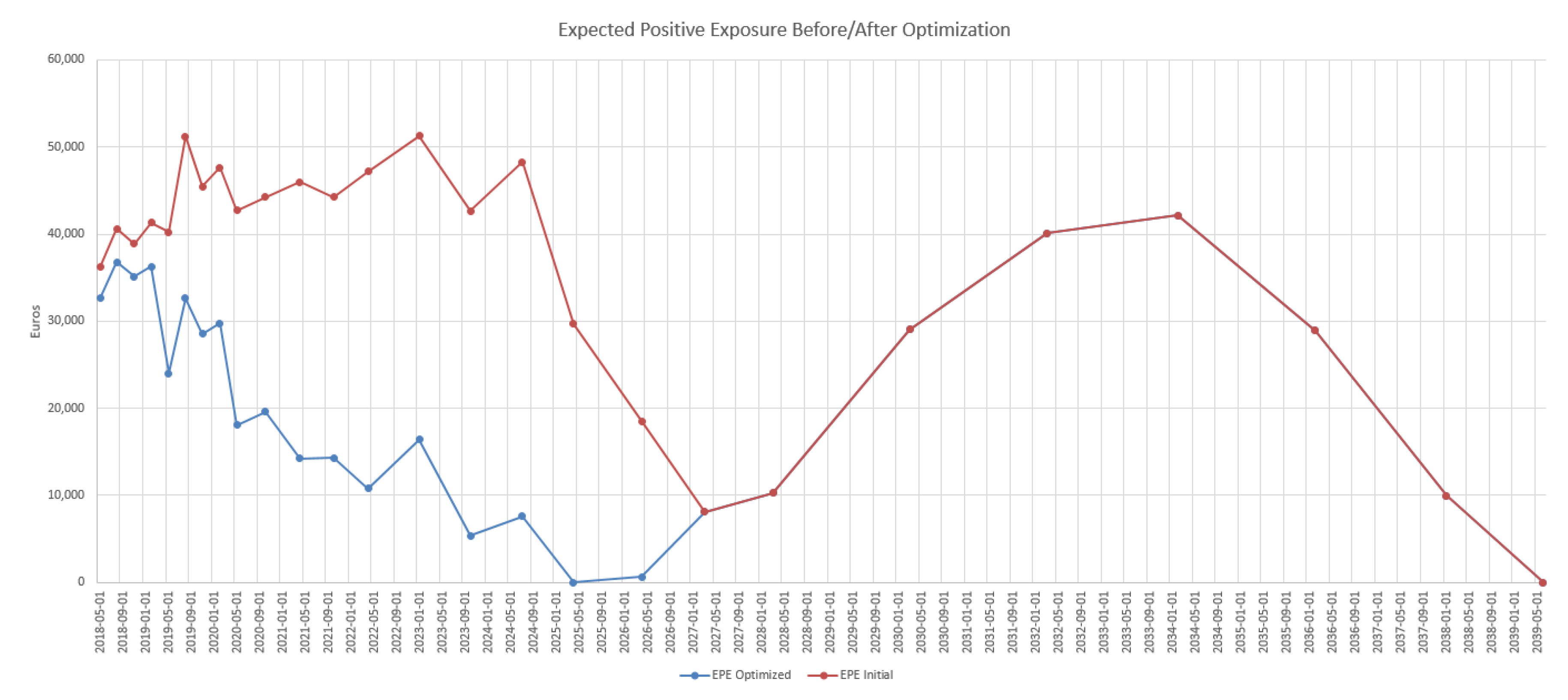
- How does the compression distort the portfolio exposure, with or without penalization?
4.1. New Deal Parameterization
- Notional: From 10 to by step of 10 dollars.
- Maturity: From 1 to 20 years by step of 1 year, 30 years and 50 years.
- Currency: Euro, US dollar, GBP or Yen.
- Direction: A binary variable for payer or receiver.
4.2. Design of the Genetic Algorithm
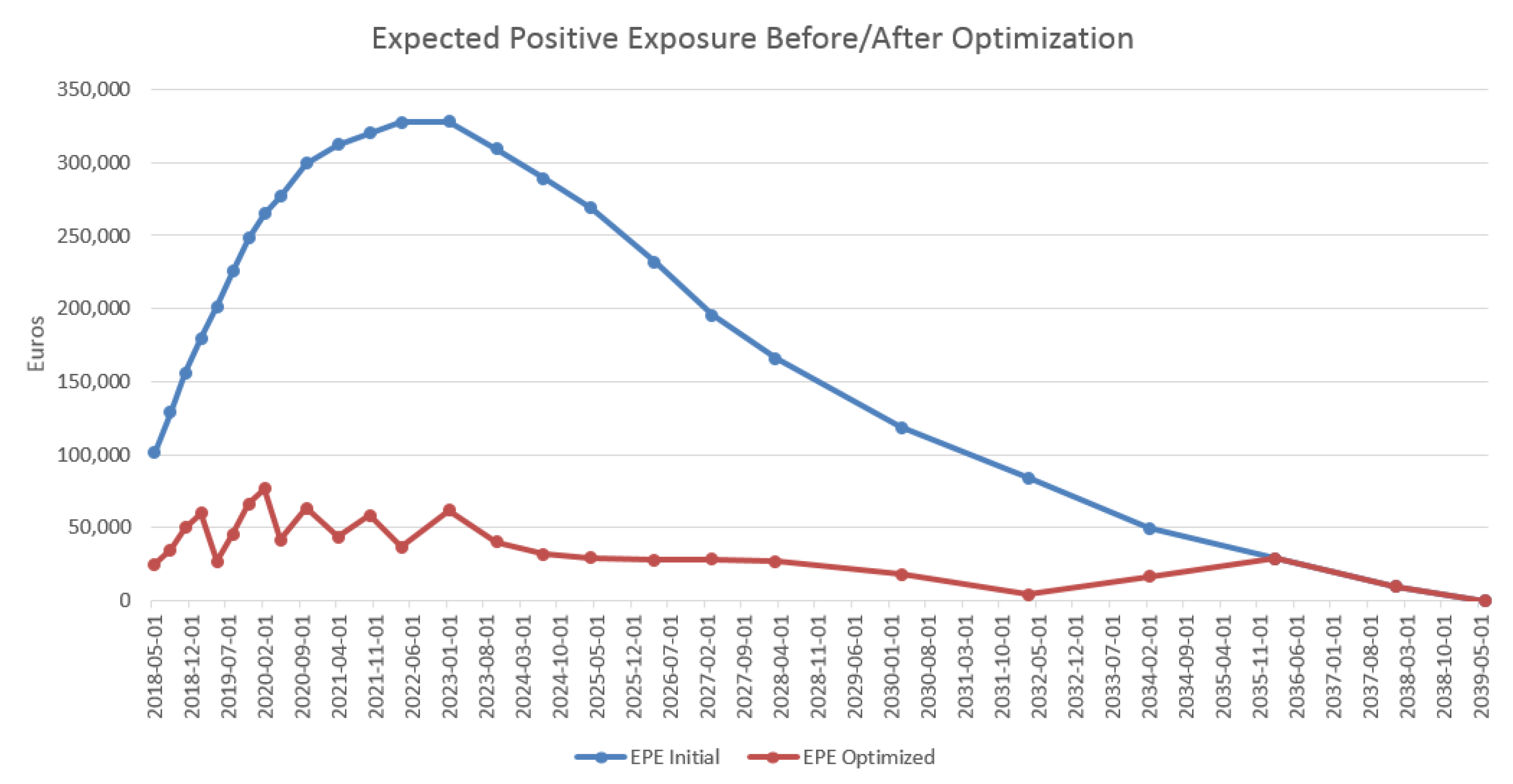
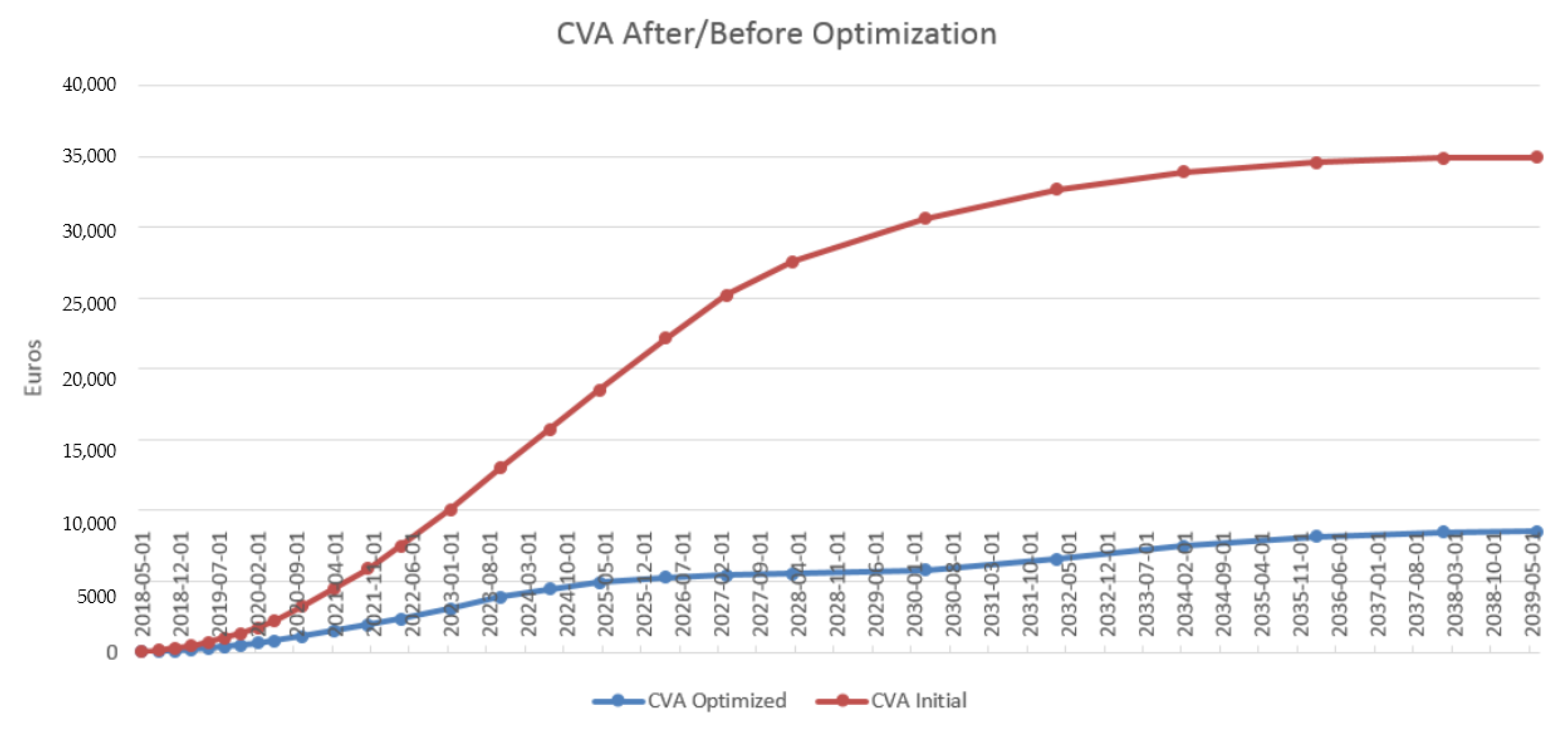
4.3. Results in the Case of Payer Portfolio Without Penalization
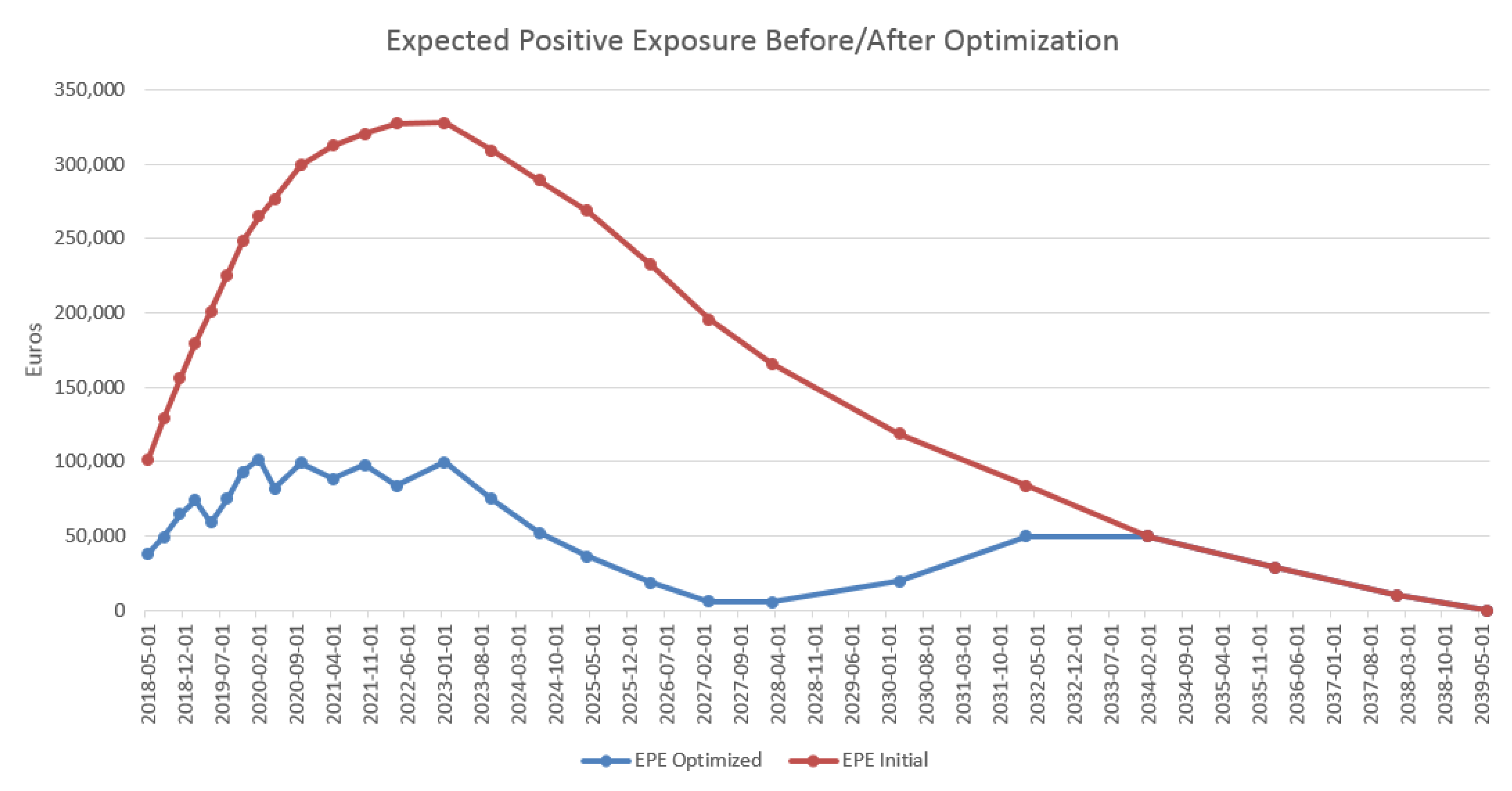
4.4. Results in the Case of Payer Portfolio With Penalization
4.5. Results in the Case of a Hybrid Portfolio With Penalization
5. Conclusions
Author Contributions
Funding
Acknowledgments
Conflicts of Interest
Abbreviations
| CDS | Credit default swap |
| CVA | Credit valuation adjustment |
| DV01 | Dollar value of an 01 |
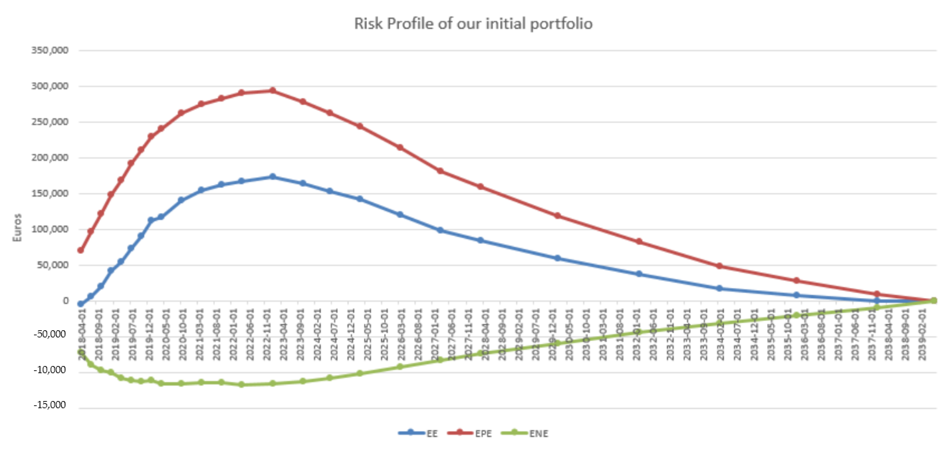
| EE | Expected exposure |
| EPE | Expected positive exposure |
| ENE | Expected negative exposure |
| FVA | Funding valuation adjustment |
| KVA | Capital valuation adjustment |
| MtM | Mark-to-market |
| MVA | Margin valuation adjustment |
| OIS | Overnight indexed swap |
| OTC | Over-the-counter |
| XVA | Generic “X” valuation adjustment |
Appendix A. Single Point Crossover
References
- Adler, Dan. 1993. Genetic algorithms and simulated annealing: A marriage proposal. Paper presented at the IEEE International Conference on Neural Networks, San Francisco, CA, USA, March 28–April 1; pp. 1104–9. [Google Scholar]
- Albanese, Claudio, and Stéphane Crépey. 2019. XVA Analysis from the Balance Sheet. Available online: https://math.maths.univ-evry.fr/crepey (accessed on 3 August 2019).
- Albanese, Claudio, Marc Chataigner, and Stéphane Crépey. 2018. Wealth transfers, indifference pricing, and XVA compression schemes. In From Probability to Finance—Lecture Note of BICMR Summer School on Financial Mathematics. Mathematical Lectures from Peking University Series; Edited by Y. Jiao. Berlin: Springer. [Google Scholar]
- Back, Thomas. 1996. Evolutionary Algorithms in Theory and Practice: Evolution Strategies, Evolutionary Programming, Genetic Algorithms. Oxford: Oxford University Press. [Google Scholar]
- Basel Committee on Banking Supervision. 2015. Review of the Credit Valuation Adjustment Risk Framework. Consultative Document. Basel: Basel Committee on Banking Supervision. [Google Scholar]
- Bergstra, James, Rémi Bardenet, Yoshua Bengio, and Balázs Kégl. 2011. Algorithms for hyper-parameter optimization. In Advances in Neural Information Processing Systems. Cambridge: The MIT Press, pp. 2546–54. [Google Scholar]
- Blickle, Tobias, and Lothar Thiele. 1995. A Comparison of Selection Schemes Used in Genetic Algorithms. TIK-Report. Zurich: Computer Engineering and Networks Laboratory (TIK). [Google Scholar]
- Brigo, Damiano, and Frédéric Vrins. 2018. Disentangling wrong-way risk: Pricing credit valuation adjustment via change of measures. European Journal of Operational Research 269: 1154–64. [Google Scholar] [CrossRef]
- Carvalho, Delmar, João Bittencourt, and Thiago Maia. 2011. The simple genetic algorithm performance: A comparative study on the operators combination. Paper presented at the First International Conference on Advanced Communications and Computation, Barcelona, Spain, October 23–29. [Google Scholar]
- Chen, Shu-Heng. 2012. Genetic Algorithms and Genetic Programming in Computational Finance. Berlin: Springer Science & Business Media. [Google Scholar]
- Cont, Rama, and Sana Ben Hamida. 2005. Recovering volatility from option prices by evolutionary optimization. Journal of Computational Finance 8: 43–76. [Google Scholar] [CrossRef][Green Version]
- Crépey, Stéphane, and Shiqi Song. 2016. Counterparty risk and funding: Immersion and beyond. Finance and Stochastics 20: 901–30. [Google Scholar] [CrossRef]
- Crépey, Stéphane, and Shiqi Song. 2017. Invariance Properties in the Dynamic Gaussian Copula Model. ESAIM: Proceedings and Surveys 56: 22–41. [Google Scholar] [CrossRef]
- Crépey, Stéphane, Rodney Hoskinson, and Bouazza Saadeddine. 2019. Balance Sheet XVA by Deep Learning and GPU. Available online: https://math.maths.univ-evry.fr/crepey (accessed on 3 August 2019).
- Del Moral, Pierre. 2004. Feynman-Kac Formulae: Genealogical and Interacting Particle Systems With Applications. Berlin: Springer. [Google Scholar]
- Drake, Adrian E., and Robert E. Marks. 2002. Genetic algorithms in economics and finance: Forecasting stock market prices and foreign exchange—A review. In Genetic Algorithms and Genetic Programming in Computational Finance. Berlin: Springer, pp. 29–54. [Google Scholar]
- Glasserman, Paul, and Linan Yang. 2018. Bounding wrong-way risk in CVA calculation. Mathematical Finance 28: 268–305. [Google Scholar] [CrossRef]
- Goldberg, David. 1989. Genetic Algorithms in Search Optimization and Machine Learning. Boston: Addison-Wesley. [Google Scholar]
- Gregory, Jon. 2015. The xVA Challenge: Counterparty Credit Risk, Funding, Collateral and Capital. Hoboken: Wiley. [Google Scholar]
- Holland, John H. 1975. Adaptation in Natural and Artificial Systems: An Introductory Analysis with Applications to Biology, Control and Artificial Intelligence. Ann Arbor: University of Michigan Press. [Google Scholar]
- Hull, John, and Alan White. 2012. CVA and wrong way risk. Financial Analyst Journal 68: 58–69. [Google Scholar] [CrossRef]
- Iben Taarit, M. 2018. Pricing of XVA Adjustments: From Expected Exposures to Wrong-Way risks. Ph.D. thesis, Université Paris-Est, Marne-la-Vallée, France. Available online: https://pastel.archives-ouvertes.fr/tel-01939269/document (accessed on 3 August 2019).
- Janaki Ram, D., T. Sreenivas, and K. Ganapathy Subramaniam. 1996. Parallel simulated annealing algorithms. Journal of Parallel and Distributed Computing 37: 207–12. [Google Scholar]
- Jin, Zhuo, Zhixin Yang, and Quan Yuan. 2019. A genetic algorithm for investment-consumption optimization with value-at-risk constraint and information-processing cost. Risks 7: 32. [Google Scholar] [CrossRef]
- Kondratyev, Alexei, and George Giorgidze. 2017. Evolutionary Algos for Optimising MVA. Risk Magazine. December. Available online: https://www.risk.net/cutting-edge/banking/5374321/evolutionary-algos-for-optimising-mva (accessed on 3 August 2019).
- Kroha, Petr, and Matthias Friedrich. 2014. Comparison of genetic algorithms for trading strategies. Paper presented at International Conference on Current Trends in Theory and Practice of Informatics, High Tatras, Slovakia, January 25–30; Berlin: Springer, pp. 383–94. [Google Scholar]
- Larranaga, P., C. Kuijpers, R. Murga, I. Inza, and S. Dizdarevic. 1999. Genetic algorithms for the travelling salesman problem: A review of representations and operators. Artificial Intelligence Review 13: 129–70. [Google Scholar] [CrossRef]
- Li, Minqiang, and Fabio Mercurio. 2015. Jumping with Default: Wrong-Way Risk Modelling for CVA. Risk Magazine. November. Available online: https://www.risk.net/risk-management/credit-risk/2433221/jumping-default-wrong-way-risk-modelling-cva (accessed on 3 August 2019).
- Pardalos, Panos, Leonidas Pitsoulis, T. Mavridou, and M. Resende. 1995. Parallel search for combinatorial optimization: Genetic algorithms, simulated annealing, tabu search and GRASP. Paper presented at International Workshop on Parallel Algorithms for Irregularly Structured Problems, Lyon, France, September 4–6; Berlin: Springer, pp. 317–31. [Google Scholar]
- Pykhtin, Michael. 2012. General wrong-way risk and stress calibration of exposure. Journal of Risk Management in Financial Institutions 5: 234–51. [Google Scholar]
- Rios, Luis, and Nikolaos Sahinidis. 2013. Derivative-free optimization: A review of algorithms and comparison of software implementations. Journal of Global Optimization 56: 1247–93. [Google Scholar] [CrossRef]
- Snoek, Jasper, Hugo Larochelle, and Ryan Adams. 2012. Practical Bayesian optimization of machine learning algorithms. In Advances in Neural Information Processing Systems. Cambridge: The MIT Press, pp. 2951–59. [Google Scholar]
- Tabassum, Mujahid, and Mathew Kuruvilla. 2014. A genetic algorithm analysis towards optimization solutions. International Journal of Digital Information and Wireless Communications (IJDIWC) 4: 124–42. [Google Scholar] [CrossRef]
- Turing, Alan M. 1950. Computing machinery and intelligence. Mind 59: 433–60. [Google Scholar] [CrossRef]
- Verma, Rajeev, and P. Lakshminiarayanan. 2006. A case study on the application of a genetic algorithm for optimization of engine parameters. Proceedings of the Institution of Mechanical Engineers, Part D: Journal of Automobile Engineering 220: 471–79. [Google Scholar] [CrossRef]
- Young, Steven, Derek Rose, Thomas Karnowski, Seung-Hwan Lim, and Robert Patton. 2015. Optimizing deep learning hyper-parameters through an evolutionary algorithm. Paper presented at Workshop on Machine Learning in High-Performance Computing Environments, Austin, TX, USA, November 15; p. 4. [Google Scholar]
| 1 | See also, e.g., David Bachelier’s panel discussion Capital and Margin Optimisation, Quantminds International 2018 conference, Lisbon, 16 May 2018. |
| 2 | For details regarding the initial margin and the MVA, see (Crépey et al. 2019, sets. 5.2 and 6.4). |
| 3 | The underlying interest rate and FX models are proprietary and cannot be disclosed in the paper. We use a deterministic credit spread model for the counterparty, calibrated to the CDS term structure of the latter. |
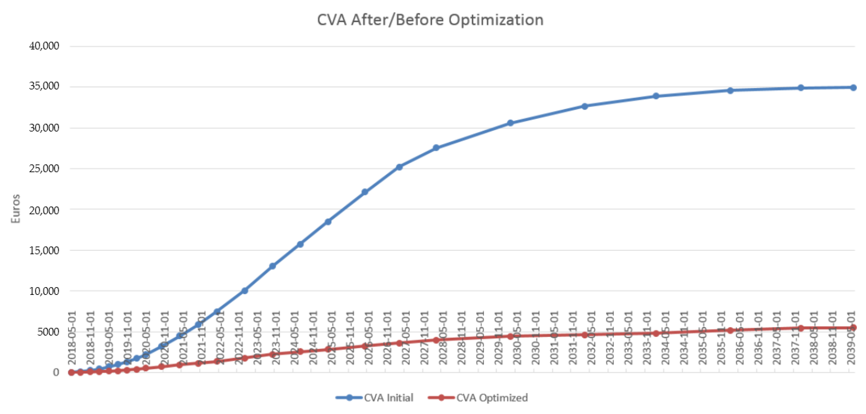
| 4 | Term structure obtained by integrating the EPE profile against the CDS curve of the counterparty from time 0 to an increasing upper bound (cf. Equation (3)). |


| Iter. | Mat. (yrs) | Not. (K€) | Rate (%) | Curr. | Pos. | CVA (€) | (in %) | |DV01|(€) |
|---|---|---|---|---|---|---|---|---|
| 0 | 10 | 4,800,000 | 1.6471 | GBP | Receive | −8019 | 23.0 | 4484 |
| 10 | 4,700,000 | 1.6471 | GBP | Receive | −7948 | 22.8 | 4390 | |
| 10 | 4,600,000 | 1.6471 | GBP | Receive | −7872 | 22.5 | 4297 | |
| 1 | 17 | 5,600,000 | 1.4623 | EUR | Receive | −17,249 | 49.4 | 8648 |
| 12 | 5,400,000 | 1.7036 | GBP | Receive | −9163 | 26.2 | 5957 | |
| 16 | 3,900,000 | 0.6377 | JPY | Receive | −8760 | 25.1 | 6137 | |
| 2 | 14 | 6,600,000 | 1.3416 | EUR | Receive | −21,680 | 62.1 | 8626 |
| 17 | 5,100,000 | 1.4623 | EUR | Receive | −19,729 | 56.5 | 7875 | |
| 17 | 5,600,000 | 1.4623 | EUR | Receive | −17,249 | 49.4 | 8648 | |
| 3 | 14 | 6,600,000 | 1.3416 | EUR | Receive | −21,680 | 62.1 | 8626 |
| 17 | 5,100,000 | 1.4623 | EUR | Receive | −19,729 | 56.5 | 7875 | |
| 17 | 5,600,000 | 1.4623 | EUR | Receive | −17,249 | 49.4 | 8648 | |
| 4 | 17 | 3,300,000 | 1.4623 | EUR | Receive | −27,300 | 78.2 | 5096 |
| 12 | 6,100,000 | 1.2203 | EUR | Receive | −25,382 | 72.7 | 6959 | |
| 11 | 5,600,000 | 1.147 | EUR | Receive | −23,009 | 65.9 | 5908 | |
| 5 | 17 | 3,300,000 | 1.4623 | EUR | Receive | −27,300 | 78.2 | 5096 |
| 12 | 6,100,000 | 1.2203 | EUR | Receive | −25,382 | 72.7 | 6959 | |
| 12 | 5,100,000 | 1.2203 | EUR | Receive | −25,264 | 72.3 | 5818 |
| Iter. | Mat. (yrs) | Not. (K€) | Rate (%) | Curr. | Pos. | CVA (€) | (in %) | |DV01|(€) |
|---|---|---|---|---|---|---|---|---|
| 0 | 10 | 4,500,000 | 1.6471 | GBP | Receive | −7790 | 22.3 | 4218 |
| 10 | 4,600,000 | 1.6471 | GBP | Receive | −7871 | 22.5 | 4311 | |
| 10 | 4,700,000 | 1.6471 | GBP | Receive | −7947 | 22.8 | 4405 | |
| 1 | 17 | 5,600,000 | 1.4731 | EUR | Receive | −16,892 | 48.4 | 8706 |
| 10 | 4,500,000 | 1.6471 | GBP | Receive | −7790 | 22.3 | 4217 | |
| 10 | 4,600,000 | 1.6471 | GBP | Receive | −7871 | 22.5 | 4311 | |
| 2 | 14 | 6,600,000 | 1.3336 | EUR | Receive | −21,888 | 62.7 | 8654 |
| 17 | 5,600,000 | 1.4731 | EUR | Receive | −16,892 | 48.4 | 8706 | |
| 17 | 6,100,000 | 1.4531 | EUR | Receive | −15,038 | 43.1 | 9466 | |
| 3 | 14 | 6,600,000 | 1.3336 | EUR | Receive | −21,888 | 62.7 | 8654 |
| 17 | 5,600,000 | 1.4731 | EUR | Receive | −16,892 | 48.4 | 8706 | |
| 9 | 4,500,000 | 0.9584 | EUR | Receive | −10,454 | 29.9 | 3945 | |
| 4 | 10 | 6,600,000 | 1.3336 | EUR | Receive | −21,888 | 62.7 | 8654 |
| 11 | 6,600,000 | 1.3999 | EUR | Receive | −18,825 | 53.9 | 9207 | |
| 17 | 5,600,000 | 1.4731 | EUR | Receive | −16,892 | 48.4 | 8706 | |
| 5 | 11 | 2,900,000 | 1.3811 | EUR | Receive | −25,059 | 71.7 | 4039 |
| 18 | 1,500,000 | 1.48 | EUR | Receive | −18,258 | 52.3 | 2442 | |
| 17 | 1,500,000 | 1.4531 | EUR | Receive | −16,553 | 47.4 | 2327 |
| Iter. | Mat. (yrs) | Not. (K€) | Rate (%) | Curr. | Pos. | CVA (€) | (in %) | |DV01|(€) |
|---|---|---|---|---|---|---|---|---|
| 0 | 1 | 6,000,000 | 0.025 | JPY | Receive | 14 | -0.2 | 609 |
| 1 | 6,100,000 | 0.025 | JPY | Receive | 14 | −0.2 | 619 | |
| 1 | 6,300,000 | 0.025 | JPY | Receive | 14 | −0.2 | 640 | |
| 1 | 8 | 1,500,000 | 0.8565 | EUR | Receive | −1905 | 29.7 | 1177 |
| 6 | 2,300,000 | 0.586 | EUR | Receive | −1166 | 18.2 | 1370 | |
| 9 | 700,000 | 1.608 | GBP | Receive | −820 | 12.8 | 595 | |
| 2 | 8 | 1,500,000 | 0.8565 | EUR | Receive | −1905 | 29.7 | 1177 |
| 6 | 2,300,000 | 0.586 | EUR | Receive | −1166 | 18.2 | 1370 | |
| 9 | 700,000 | 1.608 | GBP | Receive | −82 | 12.8 | 595 | |
| 3 | 9 | 1,900,000 | 0.9584 | EUR | Receive | −2284 | 35.6 | 1665 |
| 8 | 1,500,000 | 0.8565 | EUR | Receive | −1905 | 29.7 | 1177 | |
| 7 | 2,700,000 | 0.7225 | EUR | Receive | −1628 | 25.4 | 1865 | |
| 4 | 9 | 1,900,000 | 0.9584 | EUR | Receive | −2284 | 35.6 | 1665 |
| 8 | 1,500,000 | 0.8565 | EUR | Receive | −1905 | 29.7 | 1177 | |
| 7 | 2,700,000 | 0.7225 | EUR | Receive | −1628 | 25.4 | 1865 | |
| 5 | 9 | 1,900,000 | 0.9584 | EUR | Receive | −2284 | 35.6 | 1665 |
| 8 | 1,500,000 | 0.8565 | EUR | Receive | −1905 | 29.7 | 1177 | |
| 9 | 2,500,000 | 0.9584 | EUR | Receive | −1942 | 30.3 | 2192 |
© 2019 by the authors. Licensee MDPI, Basel, Switzerland. This article is an open access article distributed under the terms and conditions of the Creative Commons Attribution (CC BY) license (http://creativecommons.org/licenses/by/4.0/).
Share and Cite
Chataigner, M.; Crépey, S. Credit Valuation Adjustment Compression by Genetic Optimization. Risks 2019, 7, 100. https://doi.org/10.3390/risks7040100
Chataigner M, Crépey S. Credit Valuation Adjustment Compression by Genetic Optimization. Risks. 2019; 7(4):100. https://doi.org/10.3390/risks7040100
Chicago/Turabian StyleChataigner, Marc, and Stéphane Crépey. 2019. "Credit Valuation Adjustment Compression by Genetic Optimization" Risks 7, no. 4: 100. https://doi.org/10.3390/risks7040100
APA StyleChataigner, M., & Crépey, S. (2019). Credit Valuation Adjustment Compression by Genetic Optimization. Risks, 7(4), 100. https://doi.org/10.3390/risks7040100