Abstract
Solvency II requirements introduced new issues for actuarial risk management in non-life insurance, challenging the market to have a consciousness of its own risk profile, and also investigating the sensitivity of the solvency ratio depending on the insurance risks and technical results on either a short-term and medium-term perspective. For this aim, in the present paper, a partial internal model for premium risk is developed for three multi-line non-life insurers, and the impact of some different business mixes is analyzed. Furthermore, the risk-mitigation and profitability impact of reinsurance in the premium risk model are introduced, and a global framework for a feasible application of this model consistent with a medium-term analysis is provided. Numerical results are also figured out with evidence of various effects for several portfolios and reinsurance arrangements, pointing out the main reasons for these differences.
1. Introduction
The new prudential regime of the European insurance industry came in force on 1 January 2016. As well-known new risk-based Non-Life solvency capital requirements can be derived by a Standard Formula (SF), whose factor-based methodology has been calibrated on non-life insurers across European markets, regulation provides also the possibility using Undertaking Specific Parameters (USP) according to a prefixed model structure to estimate volatility. Moreover, a partial/full Internal Model (IM) may be adopted under formal approval by Member State supervisors and developed by insurers on the basis of their own specific risk profile (see ()).
Actually, most small and medium-sized insurance companies rely on SF while only the largest insurers adopt at least a Partial IM, so that the financial strength of the European insurance market can be ensured by a reasonable implementation and calibration of the standard model. By examining the adequacy of the methodology provided by Solvency II SF, some inconsistencies of the approach proposed by delegated regulation have been emphasized (see, e.g., () for non-life underwriting risk); this can lead to an over/under-estimation of the solvency capital requirement for some insurers, and it is relevant from the supervisor’s perspective.
Focusing on reinsurance recognition in the new regulation, the solution provided by Solvency II SF is based on a lognormal distribution assumption. This approach can lead to an overestimation of the risk mitigating effect of this kind of reinsurance (see ()), because it neglects the systematic component that usually affects the number of claims (see (); (); and ()), while proportional reinsurance does not affect net aggregate claims’ cost distribution, but insurers’ risk profile can change because of reinsurance pricing (see ()).
Today, collective risk modeling (see (); (); and ()) has become a popular stochastic model for premium risk in non-life insurance actuarial risk management (see ()). These models, other than being more practical, have more feasibility to incorporate a classical risk-mitigating technique such as reinsurance, modeling its impact on the solvency position. This approach, considering also reinsurance, can improve insurers’ consciousness of their own risk profile and business strategy on either a short-term or a medium-term time horizon (see ()).
New governance and disclosure requirements have by far been paying more attention to quantitative risk management, and they oblige insurers to assess the dynamic behavior of their main sources of risk and profitability on the basis of company’s industrial plan, as well as their interconnections (see ()). Furthermore, as a component of its risk-management system every insurer shall conduct its Own Risk and Solvency Assessment (ORSA), providing a comprehensive and complete vision of risks embedded in their business represented by the overall solvency needs, in order to assess both the present and the forward-looking solvency position of the company (see ()). Insurers should consider capital adequacy across the entire planning period, and the dynamic content is provided by the projection of future financial position including capital requirements (SCR) and Own Funds (OF), fixing a target capital ratio that insurers must not breach, in order to assess the going concern about the insurance company and opportunely planning its capital level (i.e., paying dividends).
Although, at the moment, this is far from influencing reinsurance purchasing decision of undertakings, growth of their risk appetite has recently been observed (see ()), which helps insurers make better decisions about reinsurance coverage options. For most of the European companies, risk appetite statements optimize reinsurance because they drive decisions on capital and profits. In this context, regulatory capital is the key capital measure used for reinsurance decisions, which has increased during the last decade due to the new prudential regime. Nevertheless, a lower volatility and stable profits are key drivers for reinsurance purchasing. Reinsurance mitigation is becoming an important component of insurers’ capital management strategy, driving key business decisions, such as, among others, earnings, dividend policy, and business strategy.
The impact of reinsurance in the Solvency II capital assessment should be analyzed since its effects on regulatory requirement are wide-spreading, becoming an important factor when insurers have to select a reinsurance contract. This analysis can be done through the development of an IM over a multi-year time horizon, considering all the risks with which the insurance company are dealing. More specifically, a three-year analysis should be done consistently with the insurers’ industrial plan, whose importance in terms of medium-term risk and business assumptions is effectively recognized by the new prudential regime.
In this framework, it is possible to introduce an SCR based on different time horizons and confidence levels (see ()). Other than the SCR provided by Solvency II on the basis of an event that can occur one time every two hundred years over the following twelve months, an alternative capital requirement can be introduced, based on considering an event that can occur one time in 20 years over the following thirty six months.
This work is aimed at defining an actuarial model from the short-term to the medium-term assessment of non-life insurers’ risk profile, investigating the Solvency II approach for the premium risk net of reinsurance.
In particular, in Section 2, a risk-capital model for the risk reserve of a non-life insurer in the presence of reinsurance is given. Section 3 describes the structure of the Solvency II regime for non-life insurance, focusing on premium risk net of reinsurance. Finally, in Section 4, numerical results are reported by focusing on the terms of solvency ratio, and in particular on the solvency capital requirements calculated by either SF or our simplified IM, incorporating reinsurance. In Section 5, we investigate the impact of two alternative portfolio mixes by a numerical analysis of the differences between these two mixes and the original one. Section 6 extends this framework for a medium-term risk profile assessment consistent with the ORSA exercise. Section 7 develops the multi-year solvency model and tries to extend the definition of the capital requirements on a medium-term perspective as well.
2. A Model in Order to Assess Risk Profile of Non-Life Insurers in Presence of Reinsurance
In classical risk theory literature stochastic risk reserve (net of reinsurance) at the end of year t using the Collective Risk Model (CRM) is given by the relation:
where the big square bracket represents the random variable (r.v.)1 of a one-year technical result for the period , evaluated at the end of year , as the difference between insurance and reinsurance results. Gross earned premiums , the stochastic aggregate claims amount of year t related to new business2 and general and acquisition expenses , with Lines of Business (LoB), are realised at the end of the year. Actually, in a calendar year insurers must take into account both earned and written premiums in their market-consistent valuation of assets and liabilities introduced by Solvency II with the new Economic Balance Sheet, but for practical purpose it is here assumed that earned premiums are equal to the written premiums3. Neither dividends nor taxation are considered in the model.
With regard to the original insurer’s portfolio, for each LoB the initial gross written premiums (GWP) are composed by gross risk premiums , safety loadings applied as a quota (constant) of the gross risk premiums and the expenses loading as a (constant) coefficient applied on the GWP :
Underlying assumption about expenses is that they are deterministic and then they are affected by a stochastic behaviour. In other words, in premium risk might be implicitly included also the expense risk (together with claims risk), linked to the volatility of the expense amount, whatever method is used to the standard deviation of premium risk evaluation, but here we neglect this component also because for many non-life segments it is rather negligible (because of the short term duration). It is also assumed that safety loading coefficient is kept constant over the time horizon.
In Equation (1) denotes the written premium volume ceded to reinsurer in the h-th LoB whereas and are respectively the amount of claim refunded by reinsurer and the reinsurance commissions, the latter is supposed to be equal to a (constant4) coefficient applied on the gross premium volume ceded to reinsurer . Note that either and depend on the type of reinsurance arranged as well as the reinsurer’s share . As for original portfolio, also for reinsurance written premiums composition we can obtain:
To evaluate characteristics of , we can make some assumptions about total claims cost for the h-th LoB gross and net of reinsurance. The aggregate claim amount for each LoB in original insured portfolio is given by a collective approach where is assumed to be a mixed compound Poisson process5 where claim size have expected value m and coefficient of variation (CoV) . Regarding premium risk only, both payments and reserves for claims incurred in previous years are necessarily covered by initial claims reserve and their volatility attains to reserve risk. Actually, reserving for outstanding claims is one of the central topics of modern actuarial theory and practise but it is here assumed that claims occurred in accounting year t they are finally settled in the same year and therefore no claims provision at the end of the year is needed. As for the original aggregate claim amount, as well as for reinsurer’s share , we can assume a mixed compound Poisson process:
depending on the type and the parameters of the reinsurance treaty in force.
Reinsurance treaties are often arranged on a claim by claim basis (i.e., Excess of Loss coverages); this means that each separate claim is divided between cedant and reinsurer and we have no impact on claims count (), where clearly the claim size distribution must be an unconditional expression. With regard to severity, the size of an individual claim net of reinsurance can be written as
It is possible to model gross premiums and claims separately from the impact of reinsurance on them, allowing direct assessment of the effects of different reinsurance strategies both on a company’s expected performance and solvency. Then we consider the aggregate claim amount net of reinsurance:
that is defined as stochastic insurer’s net retention. We can find main characteristics and probability distributions of claim variables net of reinsurance, and of reinsurer’s share, in order to assess risk profile of the “reinsured” insurer. The probability distribution function and the risk premium of the net aggregate claims cost can be obtained from a function of original aggregate claims amount and reinsurer’s share, given the type and the parameters of the reinsurance treaty in force. Introducing the new notation for reinsurance arrangements, risk reserve Equation (1) can be rewritten as:
where technical result net of reinsurance for the period in the square bracket can be also written as:
For their natural implementation in CRM applied on insurance business, we will moreover concentrate on two classical reinsurance strategies, the Quota Share (QS) and the Excess of Loss (XL) treaties, showing how these arrangements impact on non-life insurers’ risk profile. This kind of analysis is needed accordingly with new European insurance regulation that ask to European insurers to calculate their solvency capital requirements considering contracts arranged with reinsurers, which in turn are asked to fulfill minimum capital requirements introduced with Solvency II directive.
2.1. Quota Share
In the case of Quota Share reinsurance treaty, with insurer’s retention quota for the h-th LoB (with ) fixed for each claim (), reinsurer’s share for each claim and reinsurer total claims cost are and respectively, so that we obtain in a very trival way for the retained claims cost (6):
Written premium volume ceded to reinsurer (3) is:
whereas reinsurer commission paid by reinsurer to primary insurer is with a constant resinsurance expenses loading coefficient commonly established by reinsurer. Another way to consider commission, that is more coherent with real proportional treaty, assumes that reinsurer pays to cedant sliding commission that rewards or penalizes primary insurer according to the ex-post profitability of portfolio protected by the treaty, i.e., a random commission rate whose value depends on the observed Loss Ratio is usually introduced. Reinsurer’s safety loadings coefficient is usually fixed at the same value of the coefficient charged by the cedant (). It implies that the reinsurer may agree to fix reinsurance commission to pay back to the primary insurer which provided the business, but he accepts not to charge a different safety loadings coefficient than cedant; in this way the real reinsurance pricing process is nested in the commission rate mechanism. In other words, in Quota Share it is usually assumed that both insurer and reinsurer agree to charge the same safety loadings coefficient on risk premiums so the latter is accepting the underwriting policy of primary insurer. Indeed, they are simply sharing initial portfolio variability as well as profit achieved from the contracts in force with original policyholders. Then it is implicitly assumed that insurer and reinsurer are using same technical basis, i.e., frequency, severity, etc., in premium rating.
Gross-to-net adjustment factor for premium volume of a single LoB in the case of QS reinsurance is given by .
Consequently, equation of the insurance technical result (8) after QS reinsurance is given by:
where the term represents reinsurance pricing effect on QS treaty, applied directly on premium volume ceded to reinsurer. Usually the difference is non-negative and it assumes the value zero when reinsurer refunds entirely to primary insurer the same expenses loading coefficient charged on the original risk premium volume. With regards to safety loading coefficient, it’s decreasing by retained quota only and it derives from assumption that both cedant and reinsurer use same technical basis as described above. On the other hand, pure premium is decreasing by retention quota as well as the aggregate claims cost.
In QS treaties, moments of cedant’s share directly depends on initial aggregate claims amount since the former is a linear transformation of the latter, with proportional factor equal to the retained quota . Then basic characteristics of the cedant’s share can be computed by transforming the characteristics of the initial aggregate claim amount6.
2.2. Excess of Loss
In a per risk Excess-of-Loss (XL) treaty, signed for a single LoB7, for the projected year t reinsurer pays the excess over an agreed amount in respect of each claim , called priority, projected over the following years by the claim inflation rate (in a similar way as is rescaled over each year as afore mentioned). In the next part of this section, for sake of simplicity, we will disregard the time index t.
In this paper, we are concerned with per claim excess of loss reinsurance, where the cedant’s retention is defined for each claim in a certain group of risks, reinsurer paying the excess if a claim exceeds the retention level M, and there is no limit to reinsurer exposure. Cedant’s share of the claim is .
It is worth emphasizing that, under assumptions that the aggregate claim amount is a compound variable with claim size distribution function and that all risks are reinsured using the same retention limit M, the net aggregate claim amount is also a compound variable having the same claim number variable but with claim size d.f. that depends from the d.f. of the gross claim size:
More generally, k-th moments of the cedant’s share of a claim are given by:
consequently, risk indices of claim size distribution (see ()) are .
Moments of the reinsurer’s share can be obtained from Equation (13) as:
where . Note that value of is zero whenever the size of a claim is smaller than the retention limit M.
The main characteristics of cedant’s share in an excess of loss treaty can now be easily computed through basic characteristics of the cedant’s share of individual claims net of reinsurance .
With regard to severity, many distributions may be used for modeling cost of a single claim in actuarial practice and, among others, LogNormal and Pareto distribution are the most popular; the latter usually better fits heavy tail distribution whereas the former often represent so-called attritional claim8. On the other hand, the Solvency II framework has defined a standardized capital requirement assuming a LogNormal distribution not only for premium risk, one of the main risk factors of non-life insurance, but also for reinsurance mitigation recognition. Anyhow, the lognormal assumption is taken in our simulation model but it is not clearly failing the consistency of our general framework.
Under the assumption of LogNormality for the claim size distribution, the k-th moments of the net claim size are given by:
where is the cumulative distribution function of a r.v. LogNormal distributed with generic parameters and computed in point M. Parameters are obtained by the well-known Normal-to-LogNormal parameters changing formulas and .
Then net expected claim size can be obtained as:
in which we can fix the retention limit as where k is a multiplier of claim size standard deviation. Therefore, as for expected claim size, also net risk premium given by the formula is a concave, continuous, increasing function of retention limit M (See Figure 1).
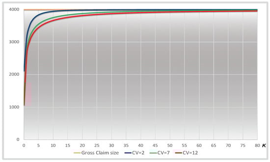
Figure 1.
Expected single claim size for different and retention limit (by multiplicative factor k).
With regard to reinsurer risk premium , it is given by the well-known relationship:
In the present model, expected value of is easily computed taking into account the LogNormal distribution with given initial parameters rescaled every year by the inflation rate i only. Reinsurance risk premium will be relatively small compared to the original risk premium if retention limit is growing up.
We compute the second moment of single claim cost in order to study its retained volatility, from formula (15) we obtain:
and consequently also net risk indices change (See Figure 2).
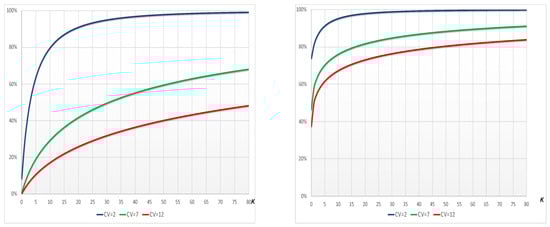
Figure 2.
Gross-to-net (Left) and (Right) for different and retention limit (by multiplicative factor k).
Then, in the case of per risk XL treaty the reinsurer’s aggregate claim amount is also a compound variable, but the number of non-zero claims is usually much smaller for a reinsurer, then stochastic claim amount charged to the reinsurer for year t is:
The retained claims cost (6) in excess of loss reinsurance is given by the following formula:
Its basic characteristics directly depend by the lowest three net retained moments about the origin introduced above:
It can be easily shown how this kind of reinsurance changes primary insurer risk profile. Under assumptions of the CRM made above, the ratio between coefficient of variation of the aggregate net and gross claims cost is:
Equation (22) for different and retention limit (by the multiplicative factor k) is reported in the next Figure 3, where all ratios between net and gross CoV of the aggregate claims cost stay between 80% and 100%, decreasing as the CoV of single claims cost of the LoB grows.
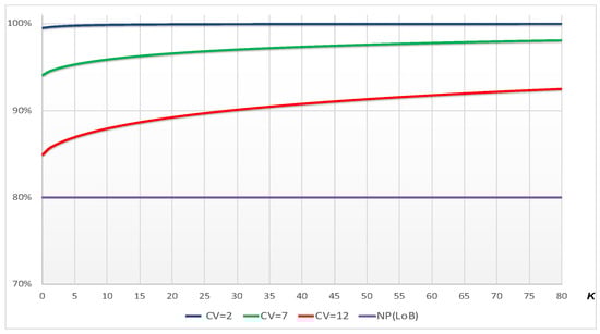
Figure 3.
Gross-to-net coefficient of variation (CoV) for different and retention limit (by the multiplicative factor k).
It emphasizes that adjustment factor for non-proportional reinsurance provided by Solvency II delegated regulation—it is 80% for some LoBs, potentially decreased by using USP for this factor—has been fixed as the lower bound of the range of y-values in order to emphasize this potential shortfall.
Now we analyze impacts of XL reinsurance on both solvency and profitability terms in Equation (7) by reintroducing segmentation between several LoBs. In the case of XL reinsurance treaty, for each LoB the safety loading coefficient is kept constant over the full time horizon and it is assumed deterministic. Safety loading coefficient in non-proportional treaties is usually greater than the one applied by insurer, and it increases as insurer’s retention limit is growing up. No explicit commissions are usually provided in case of excess of loss coverage, so that for reinsurance written premiums (3) we get:
Under the assumptions made above equation of insurance net technical result (8) after XL reinsurance can be rewritten as:
3. Solvency II Regulation for Non-Life Insurance
The new European solvency system (shortly Solvency II) has structured insurance solvency supervision according to a three-pillar approach as Basle II and for the first time an economic risk-based approach across all EU Member States has been introduced (see ()). Solvency Capital Requirement (shortly SCR) is calibrated in order to take into account all quantifiable risk to which insurance or reinsurance undertaking is exposed and its definition is based on a modular approach. The SCR must be compared with undertakings’ eligible basic Own Funds (OF), they are the available financial resources as the difference between assets and liabilities of the economic balance sheet imposed by the new regulation. Definitely, Solvency II came in force on 1 January 2016.
More specifically, in Pillar I, insurance and reinsurance undertakings will be required to “held an economic capital equal to an amount, the SCR, computed in order to ensure that ruin occurs no more often than one in every 200 cases over the following 12 months” (alternatively, a probability of default of 99.5% is considered). The European Parliament and the council of the European Union selected Value-at-Risk (9) of basic own fund of an insurance or reinsurance undertaking subject to a confidence level of 99.5% over a one-year period as measure of risk on basis of which SCR must be calculated. On the basis of model presented in Section 2 it can be written as:
Obviously, when calculating the SCR, insurance and reinsurance undertakings may take account of any financial or insurance risk-mitigation techniques they have arranged (i.e., reinsurance contracts and special purpose vehicles or financial derivatives) provided that credit risk and other risk arising from the use of such techniques are properly reflected in the calculation. Solvency II aims to appropriate recognize all risk categories an insurance company faces and all the risk mitigation techniques that insurers use to reduce exposure and thereby lower their risk capital. This marks a departure from Solvency I and its limited recognition of risk mitigation techniques.
Pillar II allows insurance and reinsurance undertakings to calculate the SCR either in accordance with the (more general) Standard Formula (SF) provided by regulation, or using, partially or fully, an Internal Model (IM). The latter is an undertaking specific method in such a way that insurers must build a model based on the own undertaking risk profile, whereas SF is a standardized calculation method since it was calibrated by insurance regulation on market average basis10. It is composed by factors reflective of the average size and performance of the portfolios of insurers in the European market. The directive describes requirements applying to insurance and reinsurance undertakings using, or willing to use, a full or partial internal model in the calculation of the SCR. Such models are subjected to prior supervisory approval on the basis of specific processes and standards, particularly regard the use test, statistical quality, calibration, validation and documentation. Actually, internal model development is one of the most important research areas in risk theory since insurers are increasingly stimulated.
Finally, Pillar III has introduced some disclosure requirements that all European insurance companies have to provide to either market and supervisors. In particular, among others, they must report the Regular Supervisory Report (RSR) and the Own Risk and Solvency Assessment (ORSA) to the supervisors, incorporating some specific analysis of undertakings risk profile and a deep assessment of business strategy on the basis of company’s industrial plan.
Now we will focus on quantitative requirements and how to calculate them. As pointed out by QIS exercise carried out from EIOPA in the last decade, for non-life insurers the underwriting risk module has the greatest impact on SCR. With regard to SF for non-life underwriting risk, delegated acts have established a unique sub-module for the joined valuation of risks related both to future claims arising during and after the period until the one-year time horizon for the solvency assessment (premium risk) and to a non-sufficient amount of technical provisions for old claims (reserve risk). The derived capital charge must be then aggregated to lapse and cat risk to quantify the capital requirement for non-life underwriting risk.
Analyzing SF in order to compare vary capital requirements evaluations, we obtain that capital requirement for premium and reserve Risk is equal to the following formula:
where is the volume measure (gross or net of reinsurance) that consists of the sum of the volume measures for premium and reserve risk of segments (LoB) involved in insurer’s business eventually decreased for the geographical diversification and is the standard deviation of ratio between aggregate claims amount of premium and reserve Risk and the volume measure, and then it is strictly related to the coefficient of variation (CoV) of their distributions.
Ignoring reserve risk, formula (26) in the case of premium risk only can be written as:
Non-life insurance segmentation between LoBs and their standard deviation have been set out by delegated acts in Annexes I and II respectively. Actually, formula (27) assumes to measure the distance between the 99,5% quantile and the mean of the probability distribution of aggregate claims amount by using a fixed multiplier of the standard deviation equal to 311.
The standard deviation for premium risk is given by the aggregation of the L different LoBs s = using a fixed12 correlation matrix R:
Non-life insurance LoBs in Solvency II framework have been defined by Annex I of the delegated acts in a similar way as those already in force in European annual accounts legislation. For our purposes LoBs of interest, in according with EIOPA’s labeling, are defined by:
- 4) Motor Vehicle Liability insurance (MVL): obligations which cover all liabilities arising out of the use of motor vehicles operating on land;
- 5) Other Motor insurance (OM): obligations which cover all damage to or loss of land vehicles;
- 8) General Liability insurance (GL): obligations which cover all liabilities other than those in the LoB 4.
In this evaluation, risk mitigation effect of proportional and non-proportional reinsurance is recognized. Generally, an insurer takes out a reinsurance cover for his insurance portfolio to increase his underwriting capacity decreasing the variation of aggregate claims cost and consequently his probability of ruin; in other words insurers adopt insurance risk-mitigation techniques in order to decrease their risk of insolvency. All these practises have been opportunely considered by new European insurance solvency system, and in delegated acts regulator has provided a suitable formula in order to take into account reinsurance as a risk-mitigation technique in new insurance solvency capital requirements. The net standard deviation of the h-th LoB in vector s of Equation (29) according to Solvency II is given by:
where gross volatility factors are showed in the next Table 1 for the three important LoBs introduced above which will be uses later in this paper for our numerical analysis:

Table 1.
Premium Risk Volatility factors for Lines of Business (LoBs)—Delegated Acts, Annex II.
Formula (29) shows how values of gross standard deviation only for premium risk in Table 1 can be multiplied by a proportional factor in order to take into account risk mitigation effect arising from existing particular XL treaties. The calculation of the premium risk SCR in non-life underwriting risk module of the SF is based on the principle of a correction factor for the disproportionate risk reduction arising out of non-proportional reinsurance treaties they shall be considered recognizable. Notwithstanding, SF provides a factor model based on predefined standard deviations for each class of insurance and the premium volume of each LoB, a correction factor is needed to reduce the gross standard deviation to a level commensurate with the risk in case insurance undertaking has provided a suitable non-proportional treaty for its lines of business. The basic idea behind this approach is to calculate an adjustment factor which is designed to consider non-proportional reinsurance risk-absorbing effect. The non-life underwriting risk module of the SF is based on volume measures such as premiums and reserves and uses predefined standard deviations per LoB to calculate the SCR. In order to appropriately capture the risk-mitigating effect of non-proportional reinsurance, the adjustment factor is designed to lower the standard deviation. Delegated acts has set this factor out at 80% for Property, Motor Vehicle Liabilities (MVL), and General Liabilities (GL) and 100% for all other LoBs.
Following Solvency II directive, volume measure is equal to the maximum between last year and next year earned premiums plus the expected present value of future premiums after one-year for existing contracts and contracts of the following year. Delegated acts SF allows undertakings to take into account a geographical diversification of business held in different macro-geographical regions of the world, through the Herfindahl Index but it will not be taken into account in the model since it is assumed that standard insurer is representative of the Italian insurance market only. The volume measure for this risk component is based on the expected premiums earned and written during the following twelve months in order to consider new business, assuming a dynamic portfolio. Then gross premium volume which is relevant for risk capital valuation will be equal to:
while for the net volumes this value would be multiplied by a gross-to-net premium adjustment factor .
According to the risk measure at Solvency II confidence level in a one-year time horizon, the capital requirement (SCR) for premium risk could be derived through our simplified internal model introduced in Section 2, referring to the time horizon , as:
Formula (31) is recognizing expected profit/losses in the capital requirement evaluation by considering safety loadings. This approach would be not conservative if a negative safety loadings were in force and a negative technical result would be expected, implying a consequent higher risk profile.
4. Numerical Analysis for Risk Assessment Gross and Net of Reinsurance Mitigation
To show the effect of a Partial Internal Model (PIM) for premium risk in the case of reinsurance based on a CRM consistent with the framework introduced in previous Section 2, three non-life insurance companies with a different size are considered (their figures are summed up in Table 2). It is assumed that all insurers underwrite contracts in same three LoBs (MVL, OM, and GL) with the same mix of portfolio (proportions used are approximately the real proportions in the Italian insurance market for these three LoBs). In the beginning, comparison of results gross of reinsurance will allow us to describe the effects of a different portfolio dimension on the aggregate claim amount distribution and so on the capital requirement. Then, it will be possible to assess also impacts of reinsurance strategies on insurers risk profile.
Table 2.
Baseline Portfolio Mix in terms of Gross premium volumes (amounts in million of Euro).
The main parameters of CRM are in Table 3. Insurers have the same characteristics apart from expected number of claims denoting the size of Insurer. Omega is assumed to be five times larger than Tau, and ten times larger than Epsilon in terms of GWP. Omega, Tau, and Epsilon are assumed to be hypothetical insurance companies representative of the Italian insurance market, whose parameters have been calibrated by historical results observed during the last 12 years (time horizon 2006–2017) and contained in Year End balance sheets of non-life Italian insurers reported every year by Italian insurers Association (ANIA) on its website, also on an aggregate basis.
Table 3.
Parameter for Collective Risk Model (CRM) analysis of Premium Risk.
In particular, parameters calibration have been based on data from some specific sheets required by Italian insurers supervision (IVASS) and very similar to EIOPA’s Quantitative Reporting Templates related to claim processes. Standard deviation of systematic volatility () and the safety loading coefficient () are obtained by Italian market Loss Ratios and Combined Ratios. Regarding the latter, it depends by the average of empirical combined ratios observed during the previous 12 years; negative values of this coefficient represent LoBs where an average of combined ratios greater than 100% (e.g., in GL) is registered. The CoV of claim size is fixed, for each LoB, and calibrated on the basis of volatility of single claim size observed in empirical datasets of non-life insurance companies in the previous calendar years. Furthermore, a dynamic portfolio is assumed and then and , reported in Table below for the initial year for each LoB considered, will increase accordingly with annual rate of real growth g as to frequency and annual claim inflation rate i as to severity, assumed to be almost 2% and 3% respectively for all LoBs in the simulations.
Table 4 shows some features of reinsurance structures as retained quota and reinsurance commission rate for QS and attachment point, net single claim cost, and safety loading coefficient applied on reinsurer premium for XL. Furthermore, for each strategy we assume an alternative reinsurance pricing that is unfavorable for the primary insurer but more realistic.
Table 4.
Parameters of reinsurance strategies.
With respect to QS treaty, we assume that retention quota is fixed for each LoB and we investigate on the different impact given by deterministic reinsurance commissions in case they are less or equal to insurer’s expense loading. For the bottom, loss in expenses loading is represented as a percentage of expenses loading coefficient of primary insurer ( in (11)), it has been fixed at for each LoB.
For XL treaty, retention limits per LoB are equal to the sum of average claim cost and a fixed multiplier k of the standard deviation: with for MVL and GL and for OM, independently from insurer’s size. Usually this multiplier is greater when a bigger insurer is considered but at the same time a greater multiplier has been assumed for long tails LoBs as MVL and GL. Furthermore, a more realistic scenario with a reinsurer safety loading coefficient greater than primary insurer safety loading coefficient is considered taking into account the reduction in variability of the ceding company, and then for LoBs with higher (lower) we will assume an higher (lower) , this is particularly important for OM and GL. For the bottom, a favourable reinsurance pricing can be assumed because of the low reduction of variability given by XL on risks of this LoB; for the latter, where a negative safety loading coefficient has been assumed in original portfolio, we will consider a very high reinsurance safety loading coefficient.
Second scenario for both reinsurance strategies would represent a more realistic arrangement that can be achieved in reinsurance market, and we named it High scenario.
The next Table 5 reports characteristics of simulated distribution of losses for total portfolio and for each LoB, obtained using software R (R Core Team 2018, Vienna, Austria) and applying 100,000 simulations so that a stable convergence of results with exact moments can be assured. CoV and skewness of gross and net of reinsurance aggregate cost of next-year claims are figured out.
Table 5.
Coefficient of variation (CoV) and skewness of simulated distribution for each LoB (Baseline Portfolio Mix).
We have that the bigger insurer shows for several LoB a CoV not so far from value of the standard deviation of the structure variable due to a relevant diversification effect given by the size, and results put in evidence that effect of non-pooling risk is significant for OM. The presence of a size factor can be noticed by the greater increase of variability showed by LoB with high coefficient as GL of smaller companies with respect to bigger insurers.
Focusing on the reinsurance effect, proportional and non-proportional treaties affect distribution of the total claims cost in a very different way. As can be expected, QS reinsurance intuitively does not change characteristics of total claims distributions as CoV and skewness for single LoBs, while mean and standard deviation are simply scaled by the retention quota . XL reinsurance, as well-known, has different impacts on characteristics of aggregate claims cost (for each LoB) according to the magnitude of of LoB considered and it hardly changes aggregate claims cost distributions of LoBs with higher as MVL and GL (See Figure 4). Particularly, CoV and skewness of net distributions for each LoB decrease thanks to this kind of reinsurance. Nevertheless, the relative effect of XL is higher as the size of the company decreases, because of a higher pooling risk of smaller insurers.
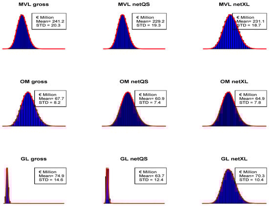
Figure 4.
Simulated distributions of Aggregate Claims Cost for Tau (for each Line of Business (LoBs)).
Aggregated distributions have characteristics very similar to MVL because of the high weight of this segment in insurers’ portfolios, and differences arise as the size of the insurer decreases, but the same comments on reinsurance effects made for a single LoB hold here. Total claims cost distribution from gross to net of QS is affected by only differences arising from applying different retentions between LoBs, and the relative effect decreases as the size of insurer grows. XL reinsurance effects on volatility and shape of aggregated distribution on single LoB basis apply also on aggregate basis. As can be seen from Table 5, the decrease in either CoV and skewness is higher for Epsilon.
The aggregation between LoBs has been derived with a simple Gaussian copula, where parameters of the copula function have been calibrated by using the correlation matrix proposed by SF in delegated acts (see Figure 5). Alternatively, we have to consider a hierarchical structure based on Archimedean copulas, more properly considering significant tail dependency between several LoBs (see (), (), and ()).
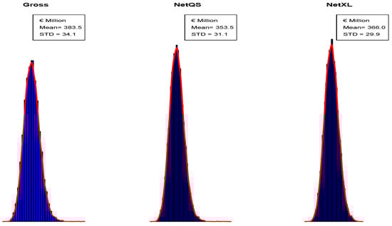
Figure 5.
Simulated distributions of Total Portfolio Aggregate Claims Cost for Tau.
Distributions of gross and net technical results are strictly related to distributions of total losses of the portfolio (see Figure 6). Mean and volatility of technical result decrease because of reinsurance, whereas distributions are characterized by a negative skewness since the r.v. is negatively affected by the aggregate claim amount distribution. It is worth mentioning that in proportional reinsurance pricing can have a significant impact on capital requirement when an IM is applied since it affects the mean of technical result distribution in such a way that an higher pricing can hardly move the whole distribution, and so the quantile 0.50%, left.
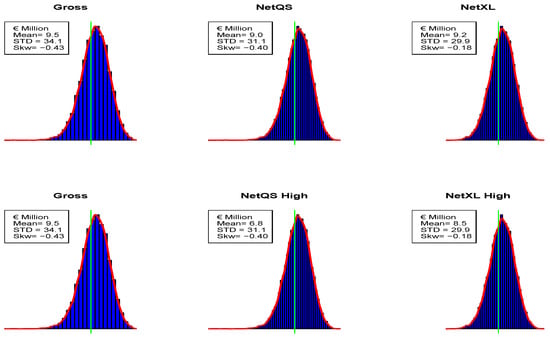
Figure 6.
Simulated Net technical result distributions for Tau (green lines on x-value 0), according to different reinsurance strategies.
Figure 7 shows instead SCR ratios obtained as capital requirement for premium risk at time t, derived using either a market-wide approach as in SF or IM introduced in the Section 2, divided by past year gross written premium (GWP), and when reinsurance is considered two alternative pricing have been considered.
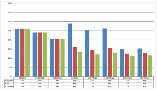
Figure 7.
Baseline portfolio mix: ratio Solvency Capital Requirement (SCR)/B.
It is worth mentioning that the main differences of SCR ratios with SF from gross to net of reinsurance arise from the related impacts on premium volume because all ratios reported are based on GWP. Furthermore, as mentioned in Section 3 SF allows insurers in some LoBs to adjust gross volatility factor in formula (29) by 20% ( for MVL and GL) when an XL treaty is in force.
On the left side of Figure 7 we report SF results, and intuitively the lack of a size factor can be deduced from differences of SCR ratios between insurers in case of IM represented on the right side, either for gross and net of reinsurance results. In the gross of reinsurance case, Epsilon have an SCR ratio calculated with IM that is approximately 2 times the ratio of Omega, while SF consider the same ratio for all insurers independently from the size.
With regard to reinsurance, the convenience of reinsurance for Epsilon can only be given by XL because of IM results lower than SCR ratios calculated with SF. On the other hand, Tau would need to implement an IM because it would decrease the SCR ratio by around 10% if compared with SF. We have also considered an unfavorable pricing denoted by letter H near to the reinsurance type (QS or XL) in Titles of columns number 6 and 8.
A lower reinsurance commission in QS results in a deterioration of ratios for all insurers considered, because translation of the distribution leads to a translation of quantile 0.50% and so of the SCR, and this effect is smoothed as the size of insurer decreases. An higher reinsurance safety loading in XL reinsurance does not heavy affect SCR ratios for all insurers because this kind of reinsurance is particularly favorable in terms of volatility, so that the negative effect on the mean is partially offset by the lower variability of the net distribution. The unfavorable effect in case of XL decreases with the size of insurer, and Omega shows bigger increase of SCR ratio because of an higher pricing than smaller insurers.
5. Numerical Analysis in Case of Different Portfolio Mix
In order to investigate impacts of some different business strategies on insurers risk profile, two others portfolio mixes will be introduced. Parameters of the model are the same introduced for baseline portfolio in previous Table 3, except of expected claims count that changes due to the different GPW in each LoB in these two different scenarios. Their differences from baseline scenario will be commented.
The first mix represents an insurer whose portfolio is Motor oriented. Mostly of the policies () are underwritten in LoBs MVL and OM, and portfolio figures are reported in the next Table 6.
Table 6.
Motor oriented Portfolio Mix in terms of Gross premium volumes (amounts in mln of Euro).
We report characteristics of simulated distribution of losses in the next Table 7, obtained by again applying 100.000 simulations to the Motor oriented portfolio using software R.
Table 7.
CoV and Skewness of simulated distribution for each LoB (Motor oriented Portfolio Mix).
Principal comments already done on characteristics of simulated distributions of each LoB in the baseline portfolio hold also for this mix, and differences arise from changes in claims count distributions parameters of the LoB considered. The characteristics of MVL are only partially affected by the different portfolio mix, with a negative effect on CoV and skewness that increase for smaller insurers. OM shows more stable results in terms of variability if compared with baseline portfolio, independent of insurer’s size, because of a low . On the other hand, for GL both CoV and skewness increase, and the relative effect is higher as the size of company decrease.
The relevant diversification effect given by size of the LoBs can be noticed by a greater increase of variability showed by LoB with high coefficient as GL of smaller companies with respect to the bigger one. Focusing on the reinsurance effect, comments of the Baseline portfolio mix hold also in this case for either QS and XL reinsurance.
Aggregated distributions have characteristics very similar to baseline portfolio because of weights between LoBs in insurers’ portfolio, but some differences arise as the size of insurer increases. Bigger insurer shows a negative impact of this mix on characteristics of total claims cost distribution gross of reinsurance, because of loss of diversification between LoBs. On the other hand, Epsilon is differently impacted by this mix because the higher GWP in LoB with lower more than compensate loss of diversification given by concentration on motor segments. In QS reinsurance, differences arising from applying different retention between LoBs because of the small weight of LoBs with lower retention as GL disappear. XL reinsurance shows a lower effect on volatility and skewness of aggregated claims cost distribution for a similar reason.
Figure 8 shows SCR ratios for Motor oriented portfolios. It can be easily seen a general decrease of all SCR Ratios because of lower CoV of LoBs within portfolio is distributed ( of the portfolio is related to MVL and OM).
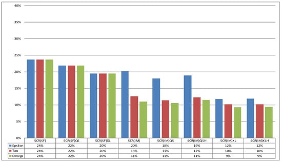
Figure 8.
Motor portfolio mix: ratio SCR/B.
Regarding differences between SF and IM, now in either gross and net of reinsurance case all insurers can implement an IM in order to save some capital. When a lower reinsurance commission in QS is considered, even a bigger insurer such as Omega has an SCR ratio close to the gross of reinsurance case because of the effect of changing proportions between LoBs into portfolios made by QS leads to loss of diversification between them. This portfolio is not particularly affected by an higher reinsurance safety loading in XL because of a lower incidence on portfolio of LoBs with higher as GL.
The second mix represents an insurer whose portfolio is Liabilities oriented. Mostly of the policies () are underwritten in LoBs MVL and GL, and portfolio figures are reported in the next Table 8.
Table 8.
Liabilities oriented Portfolio Mix in terms of Gross premium volumes (amounts in mln of Euro).
The same results in Table 7 are reported in the next Table 9, but the comments are opposite of the ones given for the Motor situation, and again differences arise from changes in claims count of LoBs OM and GL. In this case effects are smoothed because of long tails of LoBs are considered. We have a skewness not so far from value 0 due to a more relevant diversification effect given by higher weight of GL. Results show an higher volatility for OM due to lower . Also in this case QS Reinsurance intuitively does not affect the characteristics of total claims distributions for single LoBs. On the other hand XL reinsurance has a lower impact on GL because basic characteristics in gross of reinsurance case are already positively impacted by this mix if compared with the motor oriented portfolio.
Table 9.
CoV and skewness of simulated distribution for each LoB (Liabilities oriented Portfolio Mix).
Aggregated distributions have higher CoV and skewness because of the high weight of MVL and GL. Total claims amount distribution from gross to net of QS shows lower CoV and skewness because this portfolio is oriented on LoBs with lower retention, and the relative effect increases as the size of insurer grows because of the higher GWPs. Results shows the huge impact of XL reinsurance on this mix if compared with the others because of higher weight of “long tails” LoBs. Effects on volatility and skewness of net aggregated claims cost distribution increase as insurer’s size decrease and infact Epsilon shows the highest benefit in terms of CoV and skewness of all portfolio mixes and size of insurer considered.
SCR ratios for Liabilities oriented portfolios are shown in the next Figure 9. The main differences of SCR ratios between SF from gross to net to reinsurance grow in XL because of applying in Equation (29) for MVL and GL, which represent of this portfolio. There is a general increase in SCR ratios because of higher CoV of LoBs considered, and differences between SF and IM arise for smaller insurers.
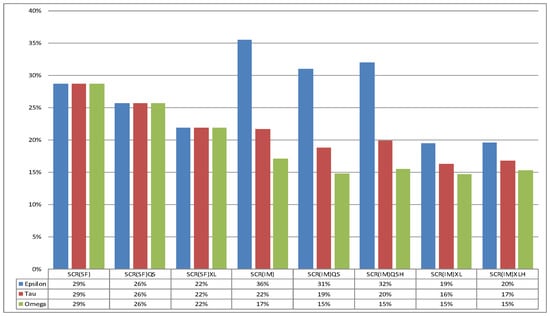
Figure 9.
Liabilities portfolio mix: ratio SCR/B.
It is worth noting the translation effect given by QS High pricing, decreasing as the size of the insurer decreases. An higher reinsurance safety loading in XL reinsurance does not heavy affect SCR ratios for all insurers because this kind of reinsurance is particularly favorable in terms of volatility, so that negative effects on the quantiles are partially offset by the lower variability of net distribution. On the other hand, the relatively more negative effect of an higher XL pricing on SCR ratios of bigger insurers increases because of the higher weight of LoBs where this kind of reinsurance has a positive impact, as in MVL and GL.
6. Medium-Term Assessment and ORSA
One of the key indicators of insurance business after Solvency II is the Solvency Ratio (SR), defined as the ratio between the OF and the SCR at time of evaluation for premium risk only. The former represents the available financial resources of an insurance company at the end of a calendar year as the sum of the initial capital and the technical result, the latter has been already commented and analyzed.
In the methodological framework given in the previous sections the SR at the time t can be computed as:
where we assume that the capital at the end of the year has been observed and so it is not stochastic, whereas is assumed to be at the time of its calculation.
As is well-known, SCR computed by either SF or IM considers only one year of new business. In the consideration of the overall solvency needs required by Solvency 2 Pillar II to be reported in the ORSA report, the risks resulting from the perspective business shall be taken into account, and then Solvency II ratio projections are made on the basis of the strategic business plan for a time horizon of 3 or 5 years. So we need a methodology in order to consider capital adequacy over the planning period, and the dynamic context as the evolution of assessment framework is provided by the projection of future financial position including capital requirements () and Own funds (), fixing a target capital ratio that insurers must not breach in order to have an appropriate capital planning. These amounts are based on multiple assumptions and parameters (combined ratios, expected dividends, etc.) and the LoB evolution shall be considered. It is worth mentioning that this method is appropriate for the business plan where there are no material change in the risk profile during the considered time horizon.
With regard to Own Funds projection, it considers at least the following elements: run-off of the inforce business, new business expected to be written over the strategic plan horizon and the market evolution (including underwriting cycles). Then the r.v. is estimated in each year t as the sum of initial own funds and the net expected profit of the year:
In the projections of the Solvency Capital Requirement over the following 3 or 5 years, the results of the last year calculation are the starting point of the calculation of the following years. SCR figures are then projected for each sub-risk and aggregated to the total SCR, using assumptions on the run-off of the inforce business and new business mix consistent with the ones used for the projection of own funds/strategic plan. We can use Equation (31), where over the following years the key drivers used to project the SCR are the premium volume and the business mix development.
The probability distributions of gross and net technical results of the valuation year and over the following 3 years are simulated and reported in the next Figure 10. Reinsurance affects yearly the gross technical result in a similar way as it does at the first year, reducing the mean and the volatility. On the other hand, distributions are characterized by a less negative skewness during the following years, because of the size factor effect given by the volume growth.
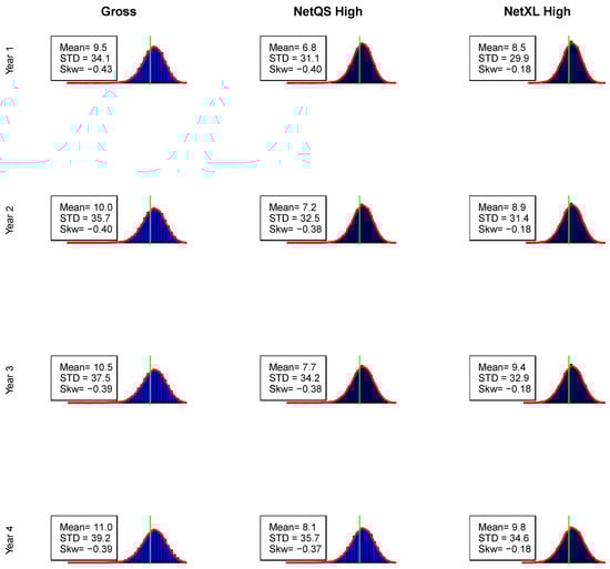
Figure 10.
Simulated Gross and Net technical result distributions for Tau (green lines on value 0), during the following 4 years—Baseline Portfolio mix (the k-th row represents distribution).
Once both OF and SCR (using IM) have been projected, the Solvency II ratio (32) for the years over the first can be easily derived by calculating the ratio between the two amounts as given above for :
When this ratio is higher than the target capital ratio over the plan period, this allows potential dividend payments each year. This is related with the Risk Appetite Framework, one of the key pillar of the risk management system, which provides risk governance tool to set risk limits and monitor risk positions.
The next Table 10 reports SR for company Tau over the following three years according to the two different reinsurance strategies already used in the paper. The initial capital has been fixed at 25% of the initial GWP (500 million euro in any scenario), so that the starting SR in the gross of reinsurance case is 135% and this value can be interpreted as the initial Risk Appetite of Tau in the Baseline scenario.
Table 10.
Solvency Ratio (SR) for Tau during the following 3 years (amounts in mln of Euro) (Baseline Ptf—20% GL).
In the baseline scenario insurer shows stable results in terms of both OF and SCR and so on SR, because of the high weight on portfolio of a stable LoB as MVL. SR increases over the years, remaining over 135% in any case, whereas net of reinsurance cases show higher values of the ratio than can be used when an higher SR would be achieved (i.e., in capital management perspective).
As can be seen in the next Table 11 and Table 12, business strategy hardly influences the solvency position of an Insurer, in such a way that a different portfolio mix impacts not only the magnitude of OF and SCR but also the behaviour of the SR over the years.
Table 11.
SR for Tau during the following 3 years (amounts in mln of Euro) (Motor Ptf—10% GL).
Table 12.
SR for Tau during the following 3 years (amounts in mln of Euro) (Liabilities Ptf—40% GL).
In particular, a portfolio oriented on the Motor segment shows better results than in the Baseline scenario, with a significant increase in the OF is only partially offset by the increase of the SCR, leading to a SR from 161% at the starting year to 200% at the end of the projection. This value increases when other reinsurance strategies are also considered, with a significant impact of XL because of an important decrease in the SCR only partially attenuated by the decrease in the OF due to the cost of the coverage.
On the other hand, a portfolio oriented on Liabilities segments shows an hard decrease of the SR over the time horizon because the lower technical results over the years do not let OF to grow as the SCR does. The SR moves from 109% at the starting year to 105% at the end of projections. Reinsurance arrangements partially attenuate this behaviour but they amplify their effects over the years of projection. Furthermore, the QS strategy negatively impacts a company’s OF that decreases in the planning period while the SCR grows, and then the fall in SR is more significant than in the other two strategies (gross and net of XL reinsurance). It is important to note that the XL strategy already helps an insurer to improve its solvency position at the starting year and over the planning period, with an increase of both OF and SCR lower than in the gross case.
Our results show how the behaviours of the SR drivers are amplified by the presence of XL and QS reinsurance, either in the positive or negative directions. They obviously achieve a reduction of the SCR because of the lower volatility of the Aggregated distribution of claims due to reinsurance. On the other hand, insurers must pay attention to the pricing structures of the reinsurance arrangements in force, where higher pricing can lead to a reduction of the technical result and so of the OF, if compared with either gross of reinsurance case and a multi-year time horizon.
7. A Medium-Term Model for the Net Risk Reserve
Now we consider risk reserve equation over several years. Starting from time 0 we develop Equation (1) in the gross of reinsurance case fixing a number of years larger than 1, generally here defined T:
where all assumptions made in the first paragraph about classical risk reserve ratio Equation (1) hold. In the big square bracket we can find the difference between the sum of the gross premium volume (net of expenses) over T years and the total claims cost over T years. The latter value has been defined as the aggregation over the T years of the sum of total claims cost of the h-th LoB, assumed to be independent. Some accuracy must be taken on the aggregation between LoBs in the case of a multi-year distribution and its impact on the solvency analysis and capital requirements in case of time dependency of claim costs.
Reinsurance effects are taken into stochastic Equation (35) in order to show how these treaties impact over insurer’s expected profit as well as its risk profile in the medium term because, usually, reinsurance treaties also use a multi-year approach.
With regard to net of QS treaty, the following risk reserve equation is obtained:
In case of XL reinsurance, the net risk reserve Equation (36) turns into:
where is the ratio between original and reinsurance risk premium ().
In the next Figure 11, Figure 12 and Figure 13 the net risk reserve ratio in a three-years analysis is reported both gross and net of Reinsurance in the Baseline portfolio mix case. With regard to reinsurance pricing structures, we analyze the more realistic situation that has been defined as Higher pricing in the previous Section 4 and Section 5. Starting values is fixed at 25% as in the previous Section 6.
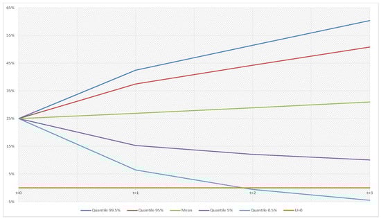
Figure 11.
, for t = 0, 1, 2, and 3 Gross of Reinsurance-Baseline portfolio mix ().
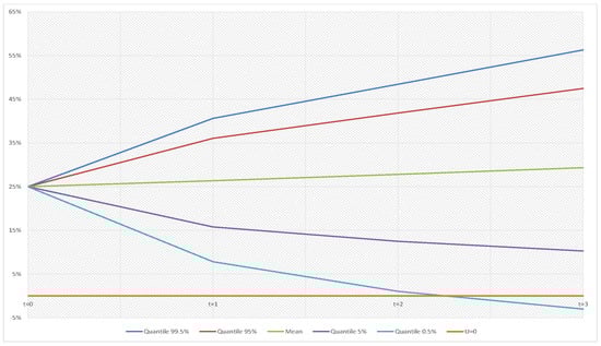
Figure 12.
, for t = 0, 1, 2, and 3 Net of Quota Share (QS) Reinsurance-Baseline portfolio mix ().
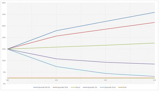
Figure 13.
, for t = 0, 1, 2, and 3 net of Excess of Loss (XL) Reinsurance-Baseline portfolio mix ().
The quantiles of risk reserve are mitigated on both sides by the presence of reinsurance, more so with XL than with QS because of the reduction of the volatility. It is worth noticing that in the last two years the 0.50% quantiles are lower than 0 either for Gross and Net QS, while it is always positive over the planning period in the case of XL. On the other hand, the mean increases during the time horizon for all the distributions considered because of the positive technical results of the years.
Once we have fixed the methodological framework underlying our medium-term model, it needs to be developed into a capital requirement calculation technique (see ()). Such analysis can be alternative as well as additional to the one carried on the previous Section 6 for a medium-term assessment of Insurance risks. Nevertheless, we can improve the methodology of Section 3 (one-year approach for the SCR) by introducing a multi-year approach to the SCR consistent with Solvency 2 framework provided by Delegated Regulation.
Equation (31) can be generalized accordingly with a confidence level in a time horizon , and then we obtain for the multi-year SCR Premium Risk:
where
Formulas (38) and (39) as in Formula (31) are recognizing expected profit/losses in the capital requirement evaluation by considering safety loadings over all of the years considered.
In practice, we can introduce an alternative SCR that considers not only a one-year but also a multi-year time horizon, as in (), taking the maximum between these quantities:
This approach permits to consider the business evolution over the company’s Industrial Plan in the calculation of the solvency capital requirement, and it would likely change consistently with business strategy the amount of capital required to insurance companies.
To show the effect of this different capital requirement, three years with a different confidence level are considered and the corresponding quantiles of risk reserve distribution for Tau are reported in Table 13. The comparison of results gross and net of reinsurance will allow to describe the effect of different capital threshold on the solvency position, while a more deep analysis on differences with other possible portfolio mix, especially with regards to quantiles, let us justify the applicability of this rule in a more realistic market context. SCR computed through Equation (39) for with and with are indicated in bold.
Table 13.
SCR for Tau according to different T and (amounts in mln of Euro).
Baseline scenario results show that in three years the company would improve its solvency position and the is greater than . This behaviour is smoothed in case of reinsurance, where QS is more effective than XL since they reduce the confidence intervals of the risk reserve distribution and they are applied on a more balanced portfolio.
A portfolio oriented on Motor segments shows better results in terms of solvency, reducing SCR and increasing differences between one-year and three-year quantiles. Reinsurance effects in terms of lower SCRs decrease if compared with the baseline portfolio mix because of the lower weight of MVL.
On the other hand, an higher weight of “long tail” LoBs in the portfolio shows the most interesting results. Here we have that is greater than only in the gross of reinsurance case. QS results are very close to them while in the case of XL we have an lower than , even if they are lower than the gross SCRs.
The results reported above show the effectiveness of different reinsurance strategies considered. QS reinsurance can be relevant for short-term to medium-term assessment of insurers’ solvency profile as it can hardly change the mean of the technical result distribution. Furthermore, differences by row between quantiles increase as the retention quota decreases, and significant attention must be paid to the pricing structure of the proportional treaties in force, even in a less risky portfolio as Motor mix. In the XL reinsurance results it has to be emphasized how this kind of reinsurance operates on lower quantiles of technical result distribution on either a one-year or multi-year time horizon. Nevertheless, it works significantly on more skewed distributions as in Liabilities oriented portfolio.
8. Conclusions
In this article we have provided a suitable PIM in order to make a short-term to medium-term assessment of a Non-Life insurance risk profile, with particular regard to the Solvency II Premium Risk. In this evaluation, reinsurance as a risk-mitigation technique has been considered in our model and its impact on our assessment opportunely reported and explained.
As numerical results evidence, business and risk strategy, as well as capital requirement methodology, may have a huge impact on the assessment of financial position of insurers under the new prudent regime of the European insurance industry. Risk mitigation techniques appear as a key driver of Non-Life insurance business as they can change risk profile over either the short-term or medium-term perspective. They impact the technical result of the year in such a way that it is important to assess how reinsurance strategies decrease the volatility, reducing the SCR given by the lower VaR, but, on the other hand, they also change the mean of distributions in different ways according to the price for risk requested by reinsurers.
At the same time, risk mitigation also appears as a key driver of Non-Life insurance management actions as it can improve business strategy and capital allocation (also in potential capital recovery plans). Different portfolio mixes change insurers’ solvency positions, and the relative effect depends on the insurer dimension and the type of reinsurance arranged. From a medium-term perspective, a non-life insurer risk profile hardly depends on the business and risk strategy, particularly in terms of insurance portfolio mix. On that point, the reinsurance again plays an active role in letting smaller insurers survive in a dynamic and competitive market context, compensating the lower level of dimension diversification in the case of XL treaty or reducing the full range of the amount at risk in the case of a Quota Share.
On the other hand, a medium-term capital requirement would ask insurers to have more capital than in a one-year time horizon. Furthermore, this effect can vary a lot between insurers with not balanced portfolios, where more volatile LoBs can deteriorate solvency position of the companies. In this framework, risk mitigation effects linked to reinsurance strategies must be assessed on either risk/return perspective trade-off as figured out in the previous section.
Author Contributions
These authors contributed equally to this work.
Funding
This research received no external funding.
Conflicts of Interest
The authors declare no conflict of interest.
Abbreviations
The following abbreviations are used in this manuscript:
| CRM | Collective Risk Model |
| GWP | Gross Written Premiums |
| SF | Standard Formula |
| IM | Internal Model |
| SCR | Solvency Capital Requirement |
| LoB | Lines of Business |
| OM | Other Motor insurance |
| MVL | Motor Vehicle Liabilities insurance |
| GL | General Liabilities insurance |
| QS(H) | Quota Share Reinsurance (High Pricing) |
| XL(H) | eXcess of Loss Reinsurance (High Pricing) |
| ORSA | Own Risk and Solvency Assessment |
| SR | Solvency Ratio |
References
- Albrecher, Hansjörg, Jozef L. Teugels, and Jan Beirlant. 2017. Reinsurance: Actuarial and Statistical Aspects. New York: Jhon Wiley & Sons. [Google Scholar]
- Cesari, Riccardo, and Valerio Arturo. 2019. Risk Management E Imprese Di Assicurazione. Aggregazione Dei Rischi E Requisiti Di Capitale Nella Nuova Vigilanza Prudenziale (Con Esempi in R). Rome: Aracne. [Google Scholar]
- Clemente, Gian Paolo, Savelli Nino, and Zappa Diego. 2014. Modelling Premium Risk for Solvency II: From Empirical Data to Risk Capital Evaluation. ICA2014 Website—Congress Papers and Presentation. Available online: https://cas.confex.com/cas/ica14/webprogram/Session6380.html (accessed on 13 June 2019).
- Clemente, Gian, Savelli Nino, and Zappa Diego. 2015. The impact of Reinsurance Strategies on Capital Requirements for Premium Risk in Insurance. Risks 3: 164–82. [Google Scholar] [CrossRef]
- Clemente, Gian Paolo, and Nino Savelli. 2017. Actuarial Improvements of Standard Formula for Non-Life Underwriting Risk. In Insurance Regulation in the European Union Solvency II and Beyond. Basingstoke: Palgrave Macmillan. [Google Scholar]
- Clemente, Gian. 2018. The effect of Non-Proportional Reinsurance: A Revision of Solvency II Standard Formula. Risks 6: 50. [Google Scholar] [CrossRef]
- Daykin, Chris D., Teivo Pentikaïnen, and Martti Pesonen. 1994. Practical Risk Theory for actuaries. In Monographs on Statistics and Applied Probability 53. London: Chapman & Hall. [Google Scholar]
- European Commission. 2015. European Commission Delegated Regulation (EU) 2015/35 Supplementing Directive 2009/138/EC(Solvency II), 10 of October 2014. Official Journal of the EU 58: 1–797. [Google Scholar]
- George, Guillaume. 2013. Insurance Risk Management & Reinsurance. Paris: ENSAE. [Google Scholar]
- Gisler, Alois. 2009. The Insurance Risk in the SST and in Solvency II: Modelling and Parameter Estimation. Helsinki: Astin Colloquium. [Google Scholar]
- International Actuarial Association. 2004. A Global Framework for Insurer Solvency Assessment. Ottawa: International Actuarial Association. [Google Scholar]
- Klugman, Stuart A., Harry H. Panjer, and Gordon E. Willmot. 2008. Loss Models: From Data to Decisions, 3rd ed. New York: Jhon Wiley & Sons. [Google Scholar]
- Sandstrom, Arne. 2011. Handbook of Solvency for Actuaries and Risk Managers: Theory and Practice. Boca Raton: CRC Press. [Google Scholar]
- Savelli, Nino. 2002. Risk analysis of a non-life insurer and traditional reinsurance effects on the solvency profile. Paper presented at 6th International Congress on Insurance: Mathematics and Economics, Lisbon, Portugal, July 15–17. [Google Scholar]
- Savelli, Nino, and Gian Paolo Clemente. 2009. Modelling Aggregate Non-Life Underwriting Risk: Standard Formula vs. Internal Model. Giornale dell’Istituto Italiano degli Attuari 72: 301–38. [Google Scholar]
- Savelli, Nino, and Gian Paolo Clemente. 2011. Hierarchical Structures in the aggregation of Premium Risk for Insurance Underwriting. Scandinavian Actuarial Journal 3: 193–213. [Google Scholar] [CrossRef]
- Venter, Gary G. 2001. Measuring value in reinsurance. Casualty Actuarial Society Forum. Available online: https://www.casact.org/pubs/forum/01sforum/01sf179.pdf (accessed on 13 June 2019).
- Willis Towers Watson. 2018. Global Reinsurance and Risk Appetite Survey Report. Available online: https://www.willistowerswatson.com/-/media/WTW/PDF/Insights/2018/07/risk-appetite-gains-momentum-in-a-changing-world.pdf (accessed on 13 June 2019).
| 1 | When a tilde is taken on a character, then it will mean that it is a random variable. |
| 2 | Claims cost of the year incorporate both payments for claims incurred during the year and the provisions for new claims (). Regarding premium risk, both payments and reserves for claims incurred in previous year are necessarily covered by initial claims reserve. Indeed, their volatility attains to reserve risk. |
| 3 | Earned premiums are the difference between written premium of the year and the one-year change in premium reserve for unearned premiums and unexpired risk . |
| 4 | Reinsurance commissions can also be stochastic: . |
| 5 | See () and () for an extensive treatment of CRM. |
| 6 | See (). |
| 7 | We avoid to refer to h-th LoB in some formulas of this subsection for practical purpose. |
| 8 | See () and EIOPA Calibration Paper on Premium and Reserve Risk. |
| 9 | It measures the potential loss in value of a risky asset or portfolio over a defined time horizon for a given confidence level. |
| 10 | Standard formula has been calibrated by EIOPA through the four Quantitative Impact Studies (QIS), carried on the whole EU insurance market on a voluntary basis by solo/group insurers. |
| 11 | It is worth mentioning that, under the assumption of a Log-Normal distribution for the aggregate claims cost, this multiplier holds only when is roughly 14.47%. It turns to overestimate capital requirement for big insurers they usually have smaller volatility coefficients. |
| 12 | Correlation parameters for two different segments are given by the correlation matrix set out in Annex IV of delegated acts. |
© 2019 by the authors. Licensee MDPI, Basel, Switzerland. This article is an open access article distributed under the terms and conditions of the Creative Commons Attribution (CC BY) license (http://creativecommons.org/licenses/by/4.0/).