Defining Geographical Rating Territories in Auto Insurance Regulation by Spatially Constrained Clustering

Abstract

Territory design and analysis using geographical loss cost are a key aspect in auto insurance rate regulation. The major objective of this work is to study the design of geographical rating territories by maximizing the within-group homogeneity, as well as maximizing the among-group heterogeneity from statistical perspectives, while maximizing the actuarial equity of pure premium, as required by insurance regulation. To achieve this goal, the spatially-constrained clustering of industry level loss cost was investigated. Within this study, in order to meet the contiguity, which is a legal requirement on the design of geographical rating territories, a clustering approach based on Delaunay triangulation is proposed. Furthermore, an entropy-based approach was introduced to quantify the homogeneity of clusters, while both the elbow method and the gap statistic are used to determine the initial number of clusters. This study illustrated the usefulness of the spatially-constrained clustering approach in defining geographical rating territories for insurance rate regulation purposes. The significance of this work is to provide a new solution for better designing geographical rating territories. The proposed method can be useful for other demographical data analysis because of the similar nature of the spatial constraint.

1. Introduction

Rate filing is an important aspect in auto insurance regulation of pricing. The purpose of rate filings is to ensure that insurance premiums offered by insurance companies are fair and exact Antonio and Beirlant (2018); Henckaerts et al. (2018); Xie and Lawniczak (2018); Harrington (1991, 1984); Leadbetter et al. (2008). Furthermore, within this process, insurance companies are required to demonstrate the appropriateness of methodologies used for pricing. This may call for rate-making benchmarks so that insurance regulators are able to judge if the proposed premiums or premium changes are justified. Among many other aspects of rate regulation, territorial rate-making is one of the most important focuses with which to deal Bajcy et al. (2003); Brubaker (2010). Essentially, this requires that insurance regulators define rating territories based on aggregated industry level loss data, without having access to more detailed information on the loss experience at the company level. Unlike insurance regulators, rating territories for an insurance company are obtained based on specific loss experience within that company and its defined territories. That is, territorial rate-making is determined using insureds’ characteristics including both individual loss experience and residential information. For instance, in Henckaerts et al. (2018), a data-driven strategy was presented by incorporating both continuous risk factors and territorial information in an auto insurance premium calculation. Since regulators have no access to such information for each individual insured and the loss experience is aggregated by regions, many of the existing clustering techniques used by insurance companies are no longer applicable to the insurance regulators. Therefore, a generalization of geographical rate-making is very necessary, and it becomes significant in insurance rate regulation. For further references on auto insurance regulation rules, readers can refer to Filing Guidelines for Automobile Insurance, Ontario, Canada. as an example, which is what this work is focused on.

Clustering analysis has now been widely used for automobile insurance pricing as a machine learning tool Jennings (2008); Samson (1986); Yao (2008); Yeo et al. (2001). It aims at partitioning a set of multivariate data into a limited number of clusters. In Samson (1986), a criterion based on least squares was used to design an efficient risk classification system for insurance companies. In Yeo et al. (2001), a data-driven approach based on hierarchical clustering was used to classify policyholders according to their risk levels, followed by a modelling of claim amounts within each group of risk. In Rempala and Derrig (2005), a finite mixture model as a clustering technique was proposed to study the claim severity in problems where data imputation is needed. More recently, in Duan et al. (2018), clustering was used to identify the low- and high-risk class of policyholders in an insurance company before a logistic regression model can be applied for risk quantification. Clustering was also used for statistical analysis of geographical insurance data in the USA, where zip codes were used as an atomic geographical rating unit Peck and Kuan (1983). However, all current research work is focusing on using clustering techniques for modelling insurance data at a company level for the purpose of having a better classification system of policyholders.

Some current research is now considering to focus on spatially-constrained clustering. In Liu et al. (2016), spatially-constrained functional clustering was used to model house prices to capture differences among heterogeneous regions. In Liao and Peng (2012), an algorithm called clustering with local search (CLS) was proposed to efficiently derive clusters for certain types of spatial data. It was demonstrated that spatially-constrained clustering is more efficient than existing methods, such as the interleaved clustering classification algorithm for spatial data. Moreover, an algorithm called constrained spectral clustering was proposed in Yuan et al. (2015) to balance the trade-off between the spatial contiguity and the landscape homogeneity of the regions. Besides spatially-constrained clustering, the newer trend on rate-making is using telematics data. In Verbelen et al. (2018), a dataset from a Belgian telematics product was used to determine insurance premiums for young drivers. Essentially, the main objective of spatially-constrained clustering is to achieve the optimality of clustering results by incorporating the spatial constraints needed so that the obtained results are more meaningful from the practical perspectives. Within the insurance area, geographical information using postal codes has been seriously considered for flood insurance pricing because the nature of insurance coverage is heavily determined by the geographical location of the insured Bin et al. (2008); Michel-Kerjan and Kunreuther (2014). There are also many insurance areas where geographical information is used, for instance in Verbelen et al. (2018); Li et al. (2005, 2010), to name a few. These research outcomes enable us to deal with rate classification problems in insurance regulation. However, unlike the type of work, for example, in Denuit and Lang (2004), where the detailed geographical information about losses was available, a regulator (e.g., in Canada) has no access to this kind of detail on geographical information. The rate-making for regulation purposes calls for an approach that is able to take this difficulty into consideration.

Another major focus of clustering is to determine the optimal number of groups. In actuarial science, the optimality of grouping is in the sense of being statistically sound, as well as satisfying insurance regulations. This is to balance the group homogeneity and the number of clusters desired to ensure that the insurance premium is fair and credible. It is particularly important when insurance premiums are regulated. However, in practice, often, the optimal groupings produced by a traditional segmentation approach are not eventually used as is, due to the credibility of data used or regulation rules. Professional judgement may be involved in making the final selection of the number of groupings for a given problem. How to minimize the gap between the suggested optimal grouping solution obtained from a statistical approach and judgemental selection is an important issue. This is also important when clustering is applied to insurance data for regulation purposes because the obtained results will provide a benchmark for an insurance company when dealing with rate-making.

The major objective of this work is to study the design of rating territories by maximizing the within-group homogeneity, as well as maximizing the among-group heterogeneity from statistical perspectives, while maximizing the actuarial equity of pure premium, as required by insurance regulation. We will consider an optimal clustering strategy for geographical loss costs, at a forward sorting area (FSA) level. In Canada, an FSA consists of the first three digits of a postal code. This implies that we treat each rating unit as a point on the map, which is simply obtained by calculating the centroid of the rating unit. Furthermore, it allows a more robust estimate of the loss cost for a given territory as it consists of higher volumes of risk exposures (i.e., number of vehicle years). Since the boundary of the geographical rating unit is not known, a spatially-constrained clustering is proposed. To ensure that the contiguity constraint was satisfied, the method of using Delaunay triangulation was used to refine the clustering results from K-means clustering. On the other hand, to determine the final optimal choice of groupings, we propose a novel approach based on entropy. A similar idea was proposed in Rodriguez et al. (2016) to help improve the homogeneity of the regions defined. In an extreme case, if the loss cost within a cluster is exactly at the same level, the average entropy of the clustering would be exactly zero. Of course, we will not expect that is going to happen in reality, but we aim for having both a small entropy measure for clustering and a relatively small number of clusters, in order to satisfy the regulatory requirement. To our best knowledge, no current research is focusing on using loss cost to classify geographical risks and using entropy to determine the optimal groupings within auto insurance rate regulation.

The layout of this paper is organized as follows. In Section 2, we briefly introduce the data used for this work. In Section 3, we discuss our proposed methods including clustering, the spatially-constrained clustering algorithm, determination of the number of clusters, as well as the entropy measure for quantifying homogeneity. In Section 4, clustering of geographical loss cost data and a summary of main results are presented. Finally, we conclude our findings and summarize remarks in Section 5.

2. Data

In this work, we will illustrate the proposed methodology applied to geographical rate classification problems in insurance regulation using a real dataset coming from an auto insurance regulator in Canada. The dataset includes the reported loss information from all auto insurance companies within the province for accident years 2009–2011. It consists of geographical information of loss in terms of postal codes, reported claim amount and earned exposures. The geographical information refers to the residential places of insured drivers who had reported the loss, rather than the place where the insured suffered the accident. This is because that insurance regulation does not keep track of the details of how loss has happened. The reported loss is the projected ultimate loss, and they are losses from all coverages. The earned exposures refer to the total number of insured vehicles within a year. In this dataset, we first retrieved all postal codes that are associated with the same FSA. For each FSA, the postal codes were further geo-coded using a geo-coder. We then used the geo-coding of postal codes within each FSA to estimate the geo-coding of the given FSA by simply taking the average of geo-coding along each dimension. Here, the geo-coding included the information of both latitude and longitude. For each FSA, the average loss cost was calculated by dividing the three-year total loss within each FSA by the three-year total number of earned exposures within the same FSA. The mean and standard deviation of loss cost by FSA were 2134 and 1553, respectively. The mean and standard deviation of earned exposures by FSA were 12649 and 9039, respectively. The obtained latitude, longitude and the associated loss cost for each FSA were the input of the clustering algorithm.

Table 1. The table summarizes data information associated with the first twenty forward sorting areas (FSA).

FSA	LossCost	Exposures	Latitude	Longitude
1	980	22,967	43.8805	−79.2639
2	1591	34,114	43.8494	−79.3258
3	3187	24,838	43.8427	−79.2709
4	1671	26,799	43.8219	−79.3945
5	1608	19,701	43.8552	−79.4008
6	1801	36,837	43.8700	−79.4391
7	1675	21,150	43.94181	−79.4549
8	2473	25,288	43.8259	−79.5869
9	2110	36,284	43.8123	−79.4493
10	1926	12,828	43.8101	−79.5054
11	1678	33,347	43.7933	−79.5797
12	1677	16,638	43.8940	−79.4224
13	3186	16,430	43.7133	−79.6427
14	606	458	43.6983	−79.6215
15	1708	15,505	43.6365	−79.6187
16	2775	8324	43.6173	−79.5816
17	1679	12,141	43.6034	−79.5944
18	2046	18,168	43.6133	−79.6467
19	2390	20,852	43.5861	−79.6103
20	2272	24,542	43.5774	−79.6300

summaries the data information for the first twenty FSA. From the table, we observe that the loss costs were different among the FSA, but some were similar to each other. Furthermore, there were some FSA containing small values of earned exposure, which may indicate that those FSA need to be re-grouped to their neighbouring FSA to obtain a larger geographical area so that the clustering is more credible.

3. Methods

In regulating auto insurance premium rates, average loss cost (or loss cost for short), i.e., pure premium, is often used as a key variable to differentiate the loss level of each designed territory. Loss cost per geographical rating unit is calculated by dividing the total loss (in terms of dollar amount) within a given rating unit by the total number of earned exposures, i.e., the total amount of time (policy year) that all policies were in effect Frees (2014). In rate classification, the territory design is to make sure that the total number of exposures in a given territory is sufficiently large so that the estimate of loss cost within a territory is credible. On the other hand, the loss cost of basic rating units within a designed territory must be similar. This implies that classification of risk in rate regulation is to find a suitable number of rating territories. These designed territories must also satisfy the contiguity constraint that is set by legal requirements. This is to ensure both the homogeneity and credibility of designed territories. Often, a larger size of rating territories or a smaller total number of rating territories is easier to satisfy the full credibility requirement, but the homogeneity requirement is not. How to achieve the homogeneity and credibility becomes the major focus of this research. Furthermore, in rate regulation, many regulators in Canada require that each territory should contain only their neighbours and cannot include any rating units that cross the boundary between territories. For example, see Wipperman (2004) and the references therein. The main reason for this constraint is due to the legal issue in rate regulation. It is often referred to as the geographical or spatial contiguity constraint, which inspires us to consider a clustering with geo-coding. Because of the contiguity constraint, we propose a two-step solution by first conducting a clustering on loss cost with the spatial contiguity constraint and then refining the results by improving the homogeneity.

3.1. Geo-Coding and Weighted Clustering

In auto insurance, territorial classification of risk is one of the important aspects due to the fact that territorial information of drivers is an important risk factor in pricing. In Canada or the USA, auto insurance loss data used for insurance rate regulation contain residential information of policyholders (i.e., postal codes), reported claim amount, reported number of claims, accident year, type of coverage, etc. For regulation purposes, the loss amount and risk exposures are aggregated by geographical area, such as postal codes. The insurance regulators then use all of the insurance loss data to further derive the loss cost by postal codes, which provides a basic risk unit (at the postal code level) for the further consideration of territorial risk classification. However, as was mentioned in the proceeding section, often, loss cost at a postal code level is less credible for regulation purposes as it may not cover enough number of reported claims. Therefore, to better reflect its nature of loss level, we have to consider a rating unit that includes a larger size of exposures so that the loss cost estimate becomes more credible. In this work, we will define FSA as a basic geographical rating unit. We will propose an approach that codes each FSA using measures of latitude and longitude. The centroid of FSA was computed by using the geo-coding of each postal code within the FSA. It was determined by averaging, respectively, the latitude values and the longitude values of the postal codes within each FSA.

In territorial pricing, it is expected that the sum of squared variation of the data among groups should be much larger than the sum of squared variation of the data within groups. This is basically to say that, in order for a territory design to be statistically sound, one should aim for a higher proportion of data variation explained by between groups and less proportion of data variation explained by within groups. Because of this, we considered the following clustering algorithm. For a d-dimensional real vector, i.e., $X_i\in R^d$, with a set of realizations {$X_1$, $X_2$, …, $X_n$}, a weighted K-means clustering (Likas et al. (2003); Kanungo et al. (2002); Burkardt (2009)) aims at partitioning of these n observations into K sets ($K\le n$), S = $\{S_1,S_2,\dots ,S_K\}$ so that the following within-cluster sum of squares (WCSS) is minimized:

$$\begin{array}{c}\hfill arg\underset{S}{min}{\displaystyle \sum _{i=1}^K\sum _{X_j\in S_i}}{\parallel X_j-{\mathit{\mu }}_i\parallel }^2,\end{array}$$

(1)

where ${\mu }_i$ is the mean point of cluster $S_i$. The weighted sum of squares is defined as follows:

$$\begin{array}{c}\hfill \parallel X_j-{\mathit{\mu }}_j{\parallel }^2={\displaystyle \sum _{l=1}^d}{w}_d{(x_{jd}-{\mu }_{id})}^2.\end{array}$$

(2)

Often each dimension of data variable $X_i$ needs to be normalized before clustering. This is because the scale of $x_{jd}$ can be reflected by the weight values. We assume that $X_i$ has been standardized. Specifically, in our case (i.e., $d=3$), ${\mathit{\mu }}_i={({\mu }_{i1},{\mu }_{i2},{\mu }_{i3})}^{\top }$ corresponds to the mean value of the ith centre of cluster and $X_j={(x_{j1},x_{j2},x_{j3})}^{\top }$ is the vector consisting of standardized loss cost $x_{j1}$, latitude $x_{j2}$ and longitude $x_{j3}$ of the jth FSA. $w_d$ is the weight value applied to the dth dimension of $X_i$. From the territory design point of review, the loss cost and geographical location are two major considerations. Given the fact that geographical location is coded in terms of latitude and longitude, which should be treated equally, so we took $w_2$ = $w_3$ = 1 (that is, latitude and longitude are equally important). We allowed $w_1$ to take different values. This idea is to control the relative importance between loss cost and geographical location using $w_1$ as a relativity. When $w_1$ = 1, the loss cost is assumed to be as important as geographical information, while taking a value greater (less) than one indicates that loss cost is treated as more (less) important than geographical information in a clustering. Notice that the K-means clustering algorithm may be affected by the choices of initial value. Different initial conditions may lead to different clustering results. To overcome this problem, we determined the optimal clustering result by simply looking at the results with different random seeds and selected the one with the minimum within-cluster sum of squares. Of course, from the theoretical perspective, it is not globally optimal. Instead, it is a sub-optimal solution because the result may depend on the initial values that we select for the clustering. Furthermore, the result was obtained under the spatial contiguity constraint. Fortunately, our investigation showed that the obtained clustering results were quite stable. The results did not depend on the initial values.

One can also use K-medoids clustering Park and Jun (2009), Sheng and Liu (2006), instead of K-means. The main difference between K-mean and K-medoids is the estimate of the centroid of each cluster. The K-means clustering approach determines each cluster centre based on the arithmetic means of each data characteristic, while the K-medoids method uses actual data points in a given cluster as a centre. However, this does not make any essential difference as we aim for grouping only. Similarly, hierarchical clustering or potentially self-organizing maps Kohonen (1990, 1997), which seeks to build a hierarchy of clusters or to build clusters based on artificial neural networks, can also be considered.

3.2. Spatially-Constrained Clustering

The K-means or K-medoids clusterings do not necessarily lead to results so that the cluster contiguity requirement is satisfied. Because of this, spatially-constrained clustering is needed in order for the obtained clusters to be spatially contiguous. Unlike the spatial clustering with boundary information, where the contiguity constraint can be achieved by making a local search of observations, we have to deal with the problem of having no boundary information, as our data suggest. That is, by clustering, we have to also determine the cluster boundary. In order to achieve this goal, the process begins with an initial clustering. The K-means clustering was applied to conduct the initial grouping of FSA with the consideration of having a similar loss cost level within the cluster. After the initial clustering, there will exist some non-contiguous points, which means that the points contained in a given cluster fall into another cluster, but not on the boundary of the cluster. For these non-contiguous points, we need to re-allocate them to their neighbouring clusters. To do so, we first searched and identified them and then re-allocated these points, one by one, to the closest point that was within a contiguous cluster and had the minimal distance to this non-contiguous point. In order to implement the allocation of non-contiguous points, an approach that is based on Delaunay triangulation Renka (1996) is proposed. To the best of our knowledge, the use of the method of using Delaunay triangulation applied to the clustering to further re-allocate the non-contiguous points is the first time this has appeared in spatial clustering of multivariate data. The use of such Delaunay triangulation is to create clusters for the given data so that contiguity constraint can be satisfied. In mathematics, a Delaunay triangulation for a set P of points in a plane is a triangulation, denoted by DT(P), such that no point in P is inside the circumcircle of any triangle in DT(P). This implies that, if a cluster is a DT, then this cluster (except the one that contains only two points in the cluster, if there exits) forms a convex hull Preparata and Hong (1977). Because the cluster is a convex hull, the clustering then satisfies the contiguity constraint. A convex hull of a set P of points is the set of all convex combinations of its points. In the case of clustering, each cluster will become one of the convex combinations. To better illustrate how a DT(P) is constructed, the following procedure is described and applied to each K for $K=1,2,\dots ,K_{max}$, where $K_{max}$ is the maximum number of clusters.

• A K-means clustering as an initial clustering was conducted so that a set of clusters can be obtained. Within the K-means, the Euclidean distance was used to capture the distance between the points to the centre of a cluster.
• Based on the initial clustering results obtained from the previous step, we searched all points that were entirely surrounded by points from other clusters. These points were denoted by non-contiguous points.
• The neighbouring point at minimal distance to the point that had no neighbours in the same cluster was found by doing a search. We refer to the associated cluster as a new cluster, which will be used for the reallocation in the next step.
• The points that have no neighbours were then reallocated to new clusters, and this process was continued.

It may be possible that reallocated points may still be isolated, which do not form a convex hull cluster. Therefore, it may be necessary for this entire routine to be repeated until no such isolated points are found in the clustering result. When this is the case, we considered these results as final.

3.3. Choice of the Number of Clusters

In clustering, the number of clusters is required before we can start to make clusters for the given multivariate data. In this work, the number of clusters refers to the number of designed territories that will be used for rate regulation. Given the fact that the selection of the number of designed territories not only depends on the results from the statistical procedure, but also will be influenced by the legal requirement, we first consider the criteria used for optimal selection from statistical perspectives and then discuss how to perform a refinement in order to meet the legal requirement. We know that finding an optimal number of clusters is challenging, especially for high-dimensional data where visualization of data by looking at all possible combinations is difficult. In order to make the optimal choice of the number of clusters, several methods including the elbow method Bholowalia and Kumar (2014), average silhouette Rousseeuw (1987) and gap statistic Tibshirani et al. (2001) have been widely used in data clustering.

The elbow method focuses on the relationship between the percentage of variance explained and the number of clusters using a visual method. The optimal choice for the number of clusters corresponds to the case that adding another cluster does not give much of decrease of the within-class variation. The major advantage of this elbow method is the ease of implementation using a graph, but the limitation is that it cannot always be unambiguously identified. A more objective approach is based on the average silhouette approach, where the silhouette width of an observation i is computed. The silhouette width is defined as:

$$\begin{array}{c}\hfill s(i)=\frac{d_1(i)-d_2(i)}{max\left\{d_1(i),d_2(i)\right\}},\end{array}$$

(3)

where $d_2(i)$ is the average distance between i and all other observations in the same cluster and $d_1(i)$ is the minimum average distance between i to other observations in different clusters. The distance measure can be Euclidean. The data observations associated with a large $s(i)$ value (almost one) correspond to the case where data are well clustered, while the data observations with a small $s(i)$ value (around zero) tend to lie between two clusters, which will cause significant overlapping and for the data observations with negative $s(i)$, probably fall into the wrong cluster.

In order to select the optimal number of clusters, we can implement the clustering by varying K from 1 $-K_{max}$. The clustering technique selected to conduct this search can be any algorithm including K-means. The average silhouette can then be computed. For a given number of clusters K, the overall average silhouette width for a clustering can be calculated as:

$$\begin{array}{c}\hfill \overline{s}(K)={\displaystyle \sum _{i=1}^n}\frac{s_K(i)}{n},\end{array}$$

(4)

where $s_K(i)$ is the silhouette width, defined in Equation (3), for a given K as the total number of clusters in clustering. The number of clusters K, which gives the largest average silhouette width $\overline{s}(K)$, was selected as the optimal choice of the number of clusters.

The gap statistic, originally proposed by Tibshirani et al. (2001), is another objective approach for determining the optimal number of clusters. This method compares the empirical data sample distribution to a null reference distribution (usually, a uniform distribution is selected as a null distribution). The optimal number of cluster K was selected such that K was the smallest value that corresponded to the statistically-significant difference of two neighbouring gap statistics. The gap statistic at a selected number of cluster K is defined as follows:

$$\begin{array}{c}\hfill \mathrm{Gap}(K)=E_N^{*}[log(W_K)]-log(W_K),\end{array}$$

(5)

where $W_K$ is the within-cluster sum of squares and $E_N^{*}[log(W_K)]$ refers to the mathematical expectation of the log-scale within-cluster sum of squares under the chosen null reference distribution and a sample size N.

As we can see from Equation (5), $E_N^{*}[log(W_K)]$ must be first determined, before we can compute the gap statistic. The computation of such an expected value was done by a re-sampling approach, where a total number of A different reference distributions was selected as null distributions, and the mathematical expectation was calculated based on the simple average of log-scale within-cluster sum of squares obtained from the simulated data using the reference distributions for different values of K, where K is from 1 $-K_{max}$ after the clustering. The log-scale within-cluster sum of squares was also computed for the observed data for each value of K after the clustering. The expected value of log-scale within-cluster sum of squares under the null distribution and its standard deviation ${\sigma }_K$ are respectively estimated as follows:

$$\begin{array}{c}\hfill E_N^{*}[log(W_K)]=\frac{1}{A}{\displaystyle \sum _{a=1}^A}log(W_{Ka})\end{array}$$

(6)

and:

$$\begin{array}{c}\hfill {\sigma }_K={\left[\frac{1}{A}{\displaystyle \sum _{a=1}^A}{\left\{log(W_{Ka})-E_N^{*}[log(W_K)]\right\}}^2\right]}^{1/2}.\end{array}$$

(7)

For a clustering with K clusters, the result is said to be statistically significant when we have the following relationship between the gap statistics $\mathrm{Gap}(K)$ and $\mathrm{Gap}(K+1)$.

$$\begin{array}{c}\hfill \mathrm{Gap}(K)\ge \mathrm{Gap}(K+1)-{\sigma }_{K+1}\sqrt{1+1/A}.\end{array}$$

(8)

The optimal K corresponds to the minimum value of K that achieves this statistical significance. However, due to the natural complexity and high level of variability of the real data, as well as the uncertainty behind the null distributions selection process, the expected value and the standard deviation that are computed using A reference distributions may lead to a potential bias. Because of this, in practice, the optimal number of clusters determined by Equation (8) may only provide us a benchmark for further analysis. To select a suitable number of clusters more systematically, the following refined approach based on Equation (8) is proposed. From Equation (8), an equivalent form is obtained as follows.

$$\begin{array}{c}\hfill \Delta G(K)=\mathrm{Gap}(K+1)-\mathrm{Gap}(K)\le {\sigma }_{K+1}\sqrt{1+1/A}.\end{array}$$

(9)

Notice that, often, the total number of null distributions A is large. Therefore, Equation (9) suggests an optimal number can be selected as the smallest K that satisfies the fact that the corresponding incremental gap statistic is less than one standard deviation. This leads to the following simplified version of Equation (9).

$$\begin{array}{c}\hfill \Delta G(K)=\mathrm{Gap}(K+1)-\mathrm{Gap}(K)\le {\sigma }_{K+1}.\end{array}$$

(10)

As we mentioned earlier, due to the fact that the real-world data are complex and may contain a high level of variation, or other considerations such as the legal requirements of the number of territories in auto insurance rate regulation, in many practical applications of clustering including the design of rating territories, the optimal choice of the number of clusters, determined by the statistical procedure, may not be eventually used. In this case, the optimal number of clusters obtained from the statistical methods may only act as a starting point. The clustering results produced by the optimal choice of number of clusters may be further partitioned to improve the results. As we just stated, the number of clusters estimated from either the average silhouette statistic or gap statistic may be affected by the noise of data. This may lead to an underestimate of the optimal number of clusters. The results presented in Figure 4 may suggest the optimal number of clusters to be seven. However, based on the professional judgement, the total number of territories, which is 22, is currently used by the regulator. The results based on a statistical approach may be subject to its own limitation due to the fact that often, it is the case that statistical approaches are based on certain assumptions. For example, in Equation (10), we assume that standard deviation ${\sigma }_{K+1}$ can be estimated and is consistent, which means that the estimate of ${\sigma }_{K+1}$ must be stable. However, with the real data, we have no control of making sure that this is the case. On the other hand, a statistical approach does not consider other constraints that either are difficult to formulate in terms of mathematical problems or impossible to incorporate, such as the legal requirement. To further refine the results, we consider the next step by increasing the value of K and measuring the homogeneity of each cluster using entropy.

3.4. Quantifying Homogeneity and Optimal Selection of K

Suppose each element of a size of n dataset X has the same probability to be selected and it is chosen at random: the probability that this element is in cluster $S_i$ is $P(i)=\frac{\mid S_i\mid }{n}$, where $\mid S_i\mid$ is the number of elements in cluster $S_i$. This is an empirical probability to measure the likelihood of association of clusters. The entropy associated with clustering S is defined as:

$$\begin{array}{c}\hfill H(S)=-{\displaystyle \sum _{i=1}^K}P(i){log}_{2}P(i).\end{array}$$

(11)

It is a measure of uncertainty for a random partition. In the extreme cases, i.e., $K=1$ or $K=n$, we had entropy for such cases as zero as the clustering of an element is certain. In this work, we used entropy to quantify the uncertainty of each cluster. We would expect a smaller entropy measure when the variation is smaller within a cluster. In rate-making, it is expected that the loss cost should be at a similar level within each cluster. This implies that for an ideal territory design that satisfies the regulation requirements including contiguity constraint and the number of territories, the uncertainty level should be as low as possible. We measured this clustering effect, $H(S)$, using the following entropy that was applied to each cluster first. The overall clustering effect using entropy was then calculated based on the average entropy of all clusters. It is given as follows:

$$\begin{array}{c}\hfill H(S)=\frac{1}{K}{\displaystyle \sum _{i=1}^K}H(S_i)\end{array}$$

(12)

where:

$$\begin{array}{c}\hfill H(S_i)=-{\displaystyle \sum _{k=1}^{B_i}}P(k){log}_{2}P(k).\end{array}$$

(13)

$B_i$ represents the total number of bins created for constructing an empirical density function of loss cost for the ith cluster. This simple averaging does not take the number of risk exposures into account. Given the fact that different clusters may consist of different numbers of exposures, it would be more reasonable to consider credibility-weighted entropy to be a global measure of homogeneity. In (12), we may re-define the simple average as a weighted average.

$$\begin{array}{c}\hfill H(S)={\displaystyle \sum _{i=1}^K}{c}_{i}H(S_i),\end{array}$$

(14)

where $c_i$ is the weight assigned to the ith cluster and ${\sum }_{i=1}^K{c}_i=1$. The choice of $c_i$ can be the portion of the exposure for each cluster, which can be defined as $\frac{E_i}{E}$, where $E_i$ is the number of exposures within the ith cluster and $E={\sum }_{i=1}^K{E}_i$ is the total number of exposures. This is often referred to as exposure weighted in the actuarial literature; see Gavin et al. (1993); Weisberg and Tomberlin (1982). The advantage for this weighted average is that overall, the measure of homogeneity is more credible, as it will be less affected by the distribution of risk exposures across different defined geographical areas.

However, we can expect that $H(S)$ decreases with the increase of K. If we aim for a small value of $H(S)$, the number of territories K may be too large, and credibility for each territory will be low as the number of exposures becomes smaller. To overcome this difficulty, we propose a penalized entropy by including a penalty term in Equation (14), which leads to the following minimization problem of penalized entropy:

$$\begin{array}{c}\hfill arg\underset{K}{min}\left\{{\displaystyle \sum _{i=1}^K}{c}_{i}H(S_i)+\frac{{(K-K_0)}^2}{N-K-1}\right\},\end{array}$$

(15)

where $\frac{{(K-K_0)}^2}{N-K-1}$ is a penalty term. Within this penalty term, $K_0$ is a control parameter, which can be judgementally selected, and N is the number of total observations (i.e., number of FSA). The selection of $K_0$ can be based on the number of territories initially obtained by other approaches. Furthermore, it is needed, otherwise this penalty term will over-penalize the average entropy so that the selected number of groupings K will be too small. This penalty term was inspired by AICc, a version of the Akaike information criterion Sugiura (1978). With the increase of N or when K was close to $K_0$, we expected a smaller penalty. When N approached infinity, the penalty became zero. When K was further from $K_0$, the penalty was larger. The idea of this proposal is to incorporate the practical experience or regulation rules into the optimal choice of K by combining the weighted average entropy with a penalty term that characterizes the departure from the judgemental selection of the number of rating territories. From Equation (15), we know that the optimal choice of the number of rating territories is the K that minimizes the penalized average entropy.

3.5. Some Discussions

We have discussed a new approach based on the spatially-constrained clustering and used entropy to further refine the clustering results. Due to the statistical nature, this proposed method for rate classification outperformed the classical approach used in rate regulation. In rate regulation of Ontario auto insurance, the territory classification is traditionally conducted by the following two-step approach, which is mainly based on professional judgement:

• By reviewing the territory classification used first by several leading companies (i.e., companies that have larger market shares), identify the commonality of the grouping of FSA and design the new territories based on the commonality of these leading companies. For those FSA that appear in different groupings among the leading companies, they are judgementally assigned to one of their nearest neighbours. This approach has some merits due to the fact that territory is used in the pricing as a key factor, and the pricing done by the companies is usually optimized. Furthermore, the results from the leading companies are good representatives of the underlying population. Within this first step, around 50 territories were obtained, which is a similar number as the one used by the leading companies.
• Followed by the initial design of the territory, the homogeneity of designed territories is then evaluated. The common practice of defining the homogeneity of a group is based on the similar level of the loss amount. Those areas with similar loss amounts are then grouped into the same group and defined as the same risk group. Due to the fact that different territories have different levels of loss cost, as well as different levels of data variability, it is important to consider both the loss amount and its variability. The coefficient of variation (CV), which is defined by the ratio of the standard deviation to the mean of the data, was used to identify the region with completely different risk levels. The neighbouring FSA associated with a similar risk level were then combined to reduce the number of territories. The advantage of using CV is that this measure reflects a relative change of percentage of loss cost.

Comparing the proposed method with the classical method, we can see that the proposed new method is more appealing due to the fact that the design of territories is based on the statistical procedure, and it is considered to be both statistically and actuarially sound. The limitation of the proposed method is that the design of territories is based on the aggregated loss cost of FSA, while companies’ pricing may use different rating territories such as postal codes. This will cause some difficulties in the review of company rate changes.

Another key aspect that we would like to address is that designing the rating territories is an unsupervised learning problem. This is the main reason why the k-means or other related clustering techniques become useful in designing territories. We would like to point out that, although K nearest neighbours (K-NN) may be useful in achieving the contiguity in designing the rating territories, it cannot be used as K-NN works only for classification or regression problems, not for clustering. As a predictive modelling technique, K-NN requires a response variable. Potentially, loss cost may play as the role of being a response variable, and geographical information can serve as explanatory variables. When this is the case, one can only establish the relationship between loss cost and geographical location, and the prediction of loss cost at other locations where the loss cost may not be observed can be addressed. However, this does not meet our research objective. We aim for designing a geographical rating of territories, which requires a grouping of geographical locations (i.e., FSA in this work). We do not focus on prediction of the loss cost for geographical locations. The design of rating territories must take both loss cost and geographical information as input variables together for any statistical techniques that help achieve the groupings.

4. Results

In this section, we report the results by applying the proposed spatial constraint clustering method to the dataset that was discussed in the Section 2. For most of the analysis being done in this paper, the results were obtained by applying all loss cost data. However, a subset of data corresponding to a selected smaller area was created and used to investigate the effect of a weight value $w_1$ on the obtained clustering results. For this purpose, We take the values of $w_1$ from 0.5–1.6 with an incremental step of 0.1. The major findings of the obtained results are summarized in

Table 2. The table summarizes the results of the total number of clusters and the minimum size of clusters within each clustering for different weight values used.

Weight ${\mathit{w}}_{\mathbf{1}}$	Number of Clusters (K)	Minimum Size of Cluster
0.5	4	2
0.6	4	2
0.7	3	7
0.8	3	5
0.9	4	2
1.0	4	2
1.1	2	14
1.2	2	11
1.3	2	11
1.4	2	11
1.5	2	11
1.6	9	1

.

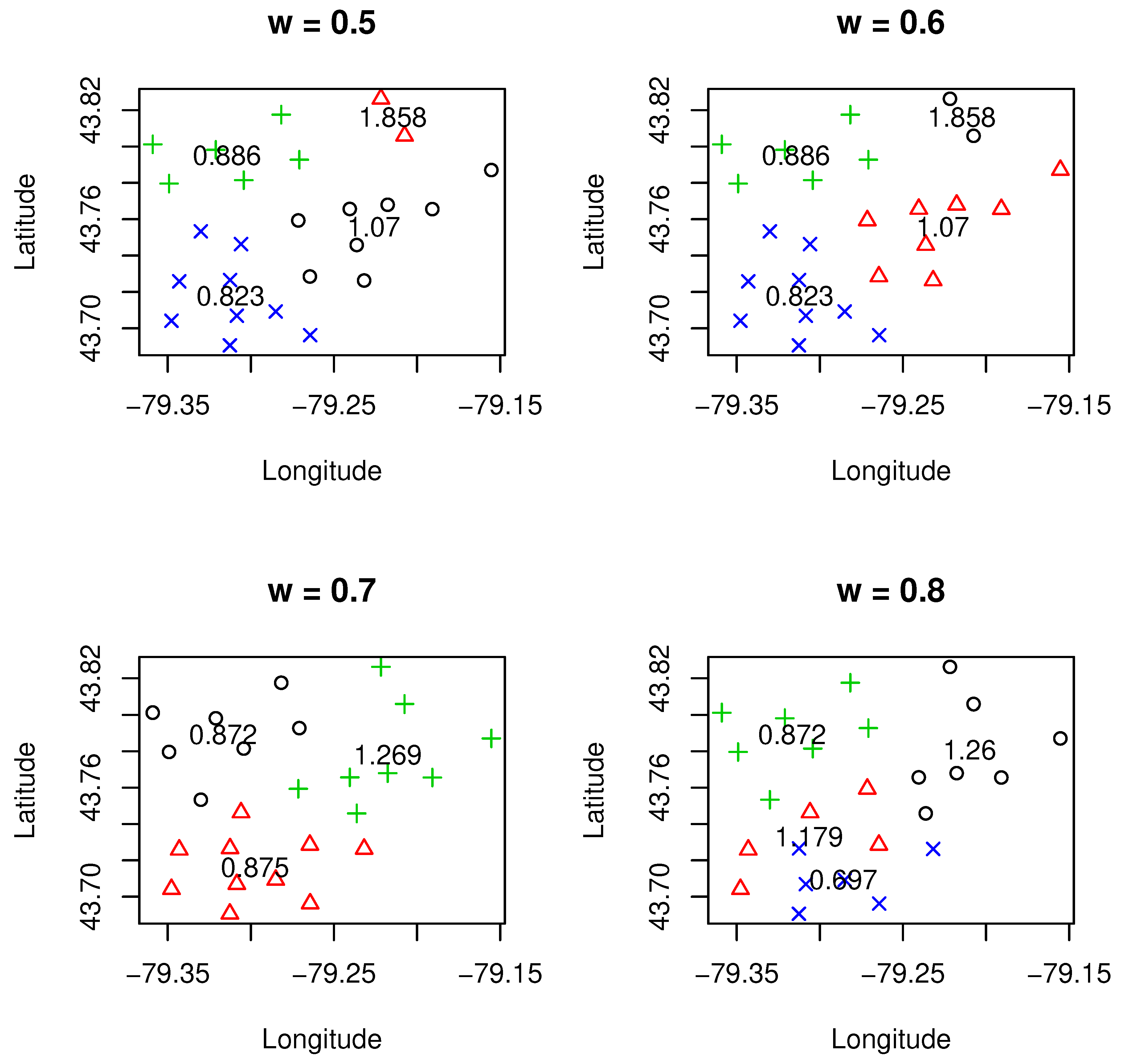
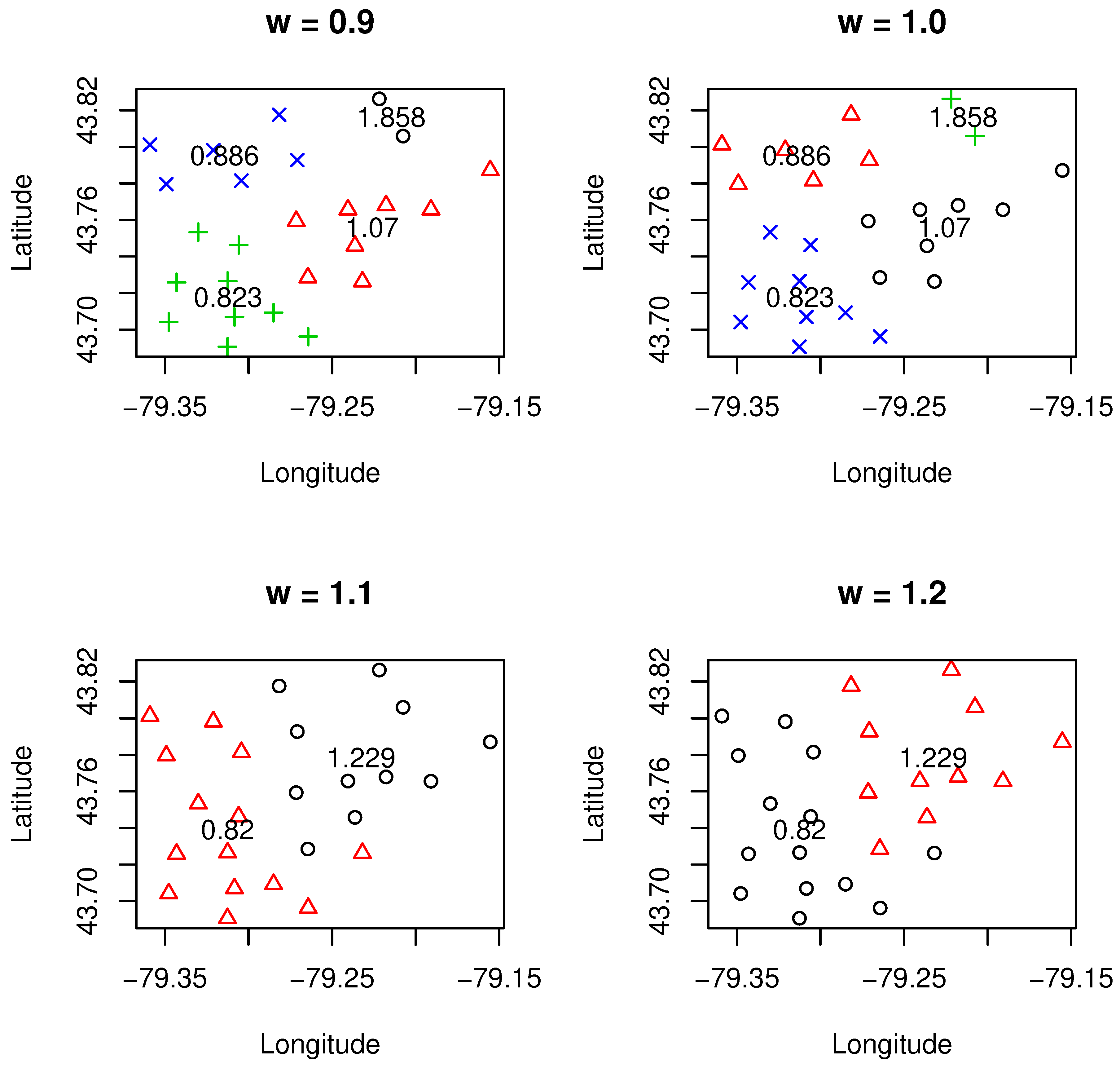
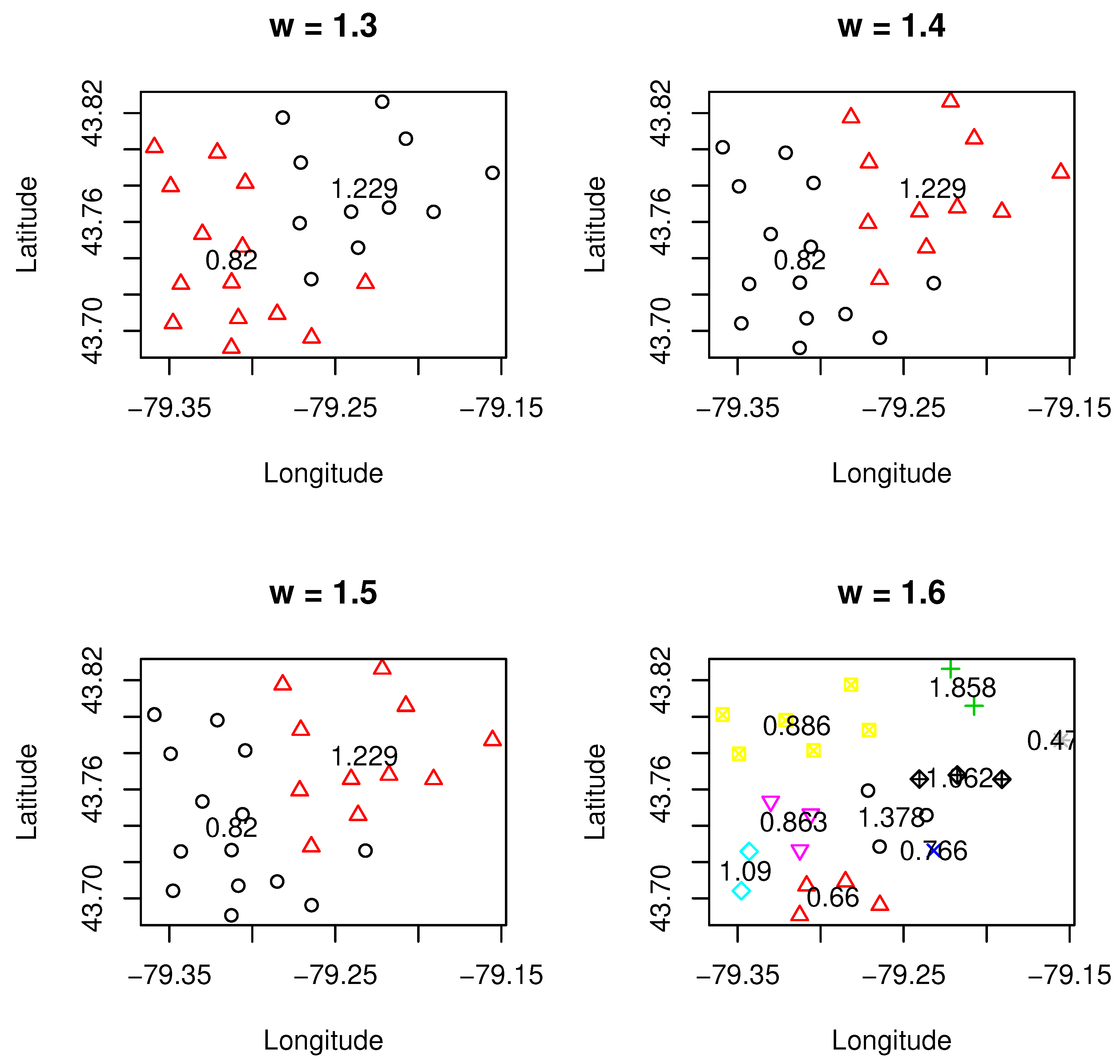
From Table 2, we can see that when $w_1$ takes smaller value than one, which implies that clustering was mainly determined by geographical information; there were more clusters retained in the final model, and the minimum size of the cluster was small (most of the results contained a cluster that had only two FSA). However, when we assigned higher weight value to the loss cost, the clustering results appeared to be more credible as only two clusters were needed and there were more FSA contained in the clusters. The result was dramatically changed when the weight value was higher than 1.6. In this case, there were too many clusters being produced, and the sizes of clusters were all much smaller. This finding may suggest that balancing the loss cost and geographical location well is important to ensure a reasonable total number of clusters. This help improve the credibility of the design of the territory.

Figure 1, Figure 2 and Figure 3 display the detailed results of clustering under different values of $w_1$. The clustering results were under the selection of the optimal number of clusters using the methods we discussed above. One can see from these results that different values of $w_1$ led to a different number of clusters. Roughly speaking, with smaller values of $w_1$ than one or sufficiently larger than one (i.e., $w_1$ = 1.6), the number of clusters tended to be higher. This implies that when certain data characteristics such as loss cost or geographical information are emphasized, more clusters are needed in order to reach an overall balance on the homogeneity of clusters. These can be observed from both Figure 1 and Figure 3, where more clusters are associated with either a smaller value of $w_1$ or a larger value of $w_1$ (i.e., $w_1$ = 1.6).

Another important point we need to make is that the relativity for the designed clusters, which is defined as the ratio of average loss cost within a cluster and overall average loss cost for all clusters (weighted by exposures), is quite sensitive and is affected by the weight value $w_1$. To achieve the overall balance within a clustering, if either geographical information or loss cost needs to be emphasized for certain reasons, the underlying cost is that there might exist certain clusters in which their relativities need to be changed significantly. This is due to the new boundaries of clusters created, and inclusion or exclusion of a particular FSA may lead to a significant change on the relativity of loss cost. We also observed that there was a significant change in the number of clusters from 2–9 when $w_1$ moved from 1.5–1.6. Further research is needed to better understand this phenomenon. One possible reason for such change may be due to the existence of phase transition, a common phenomenon in physics. As regards the credibility, it turned out that it was more credible for the clustering when $w_1$ was higher than one, which implies that when the loss cost was emphasized, the clustering results turned into being more credible.

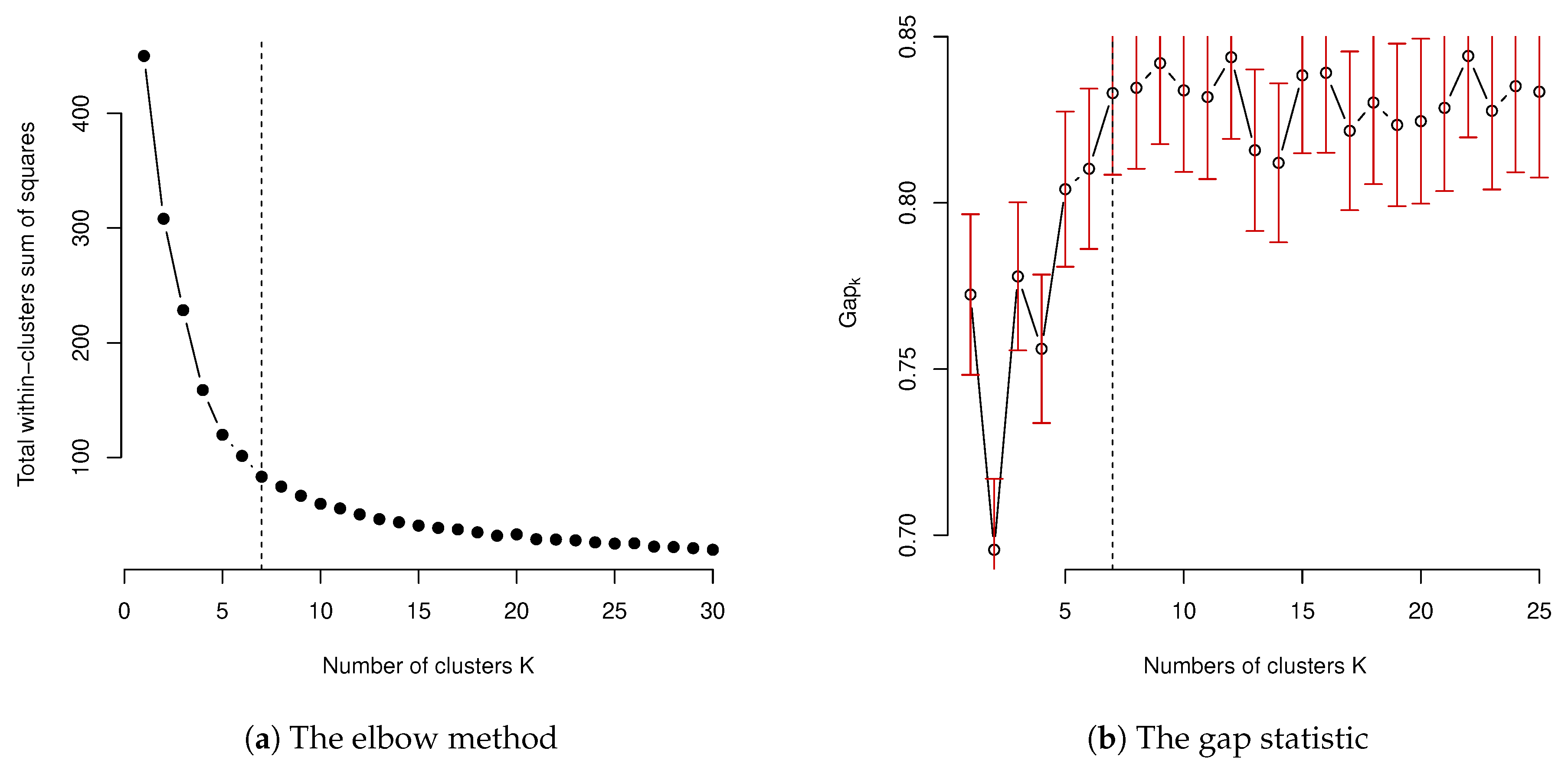
As we mentioned in Section 3, in order to produce the clustering results, we have to make the optimal choice of the number of clusters needed in the final clustering results statistically. In order to illustrate this, the results of using elbow method and the gap statistic method are presented and displayed in Figure 4. The result of using average silhouette is not presented, but it was quite similar to the result of using the elbow method. For the input data with scaling, the elbow method suggested seven clusters in the final model. The choice of the number of clusters for the elbow method was based on the smallest K, which lead to a statistically-insignificant decrease of the within-group total sum of squares, while the number of clusters by the gap statistic was selected at the K value when $\Delta G$ was larger than ${\sigma }_{K+1}$. However, when this choice of using gap statistic was applied, the gap statistic was only suggested to be one for the number of clusters, which has no practical meaning as it suggests that there is no need to conduct a clustering study for the given data and leads to no design of territory. This undesired result may be because of the heavy distortion caused by the the estimate of gap statistic $G(k)$, as well as the associated standard deviation ${\sigma }_{K+1}$. This suggests that a more suitable choice of the number of clusters K should be determined by focusing on the overall pattern of the resulting gap statistic, instead. The selection of K should be based on the signal component of $G(K)$ and select the one that first approaches the stable value of the gap statistic. When this approach is taken, a similar number was obtained to the ones obtained by the elbow method. In the choice of optimal number of clusters, the average silhouette method also gave a similar result to both the elbow method and gap statistic.

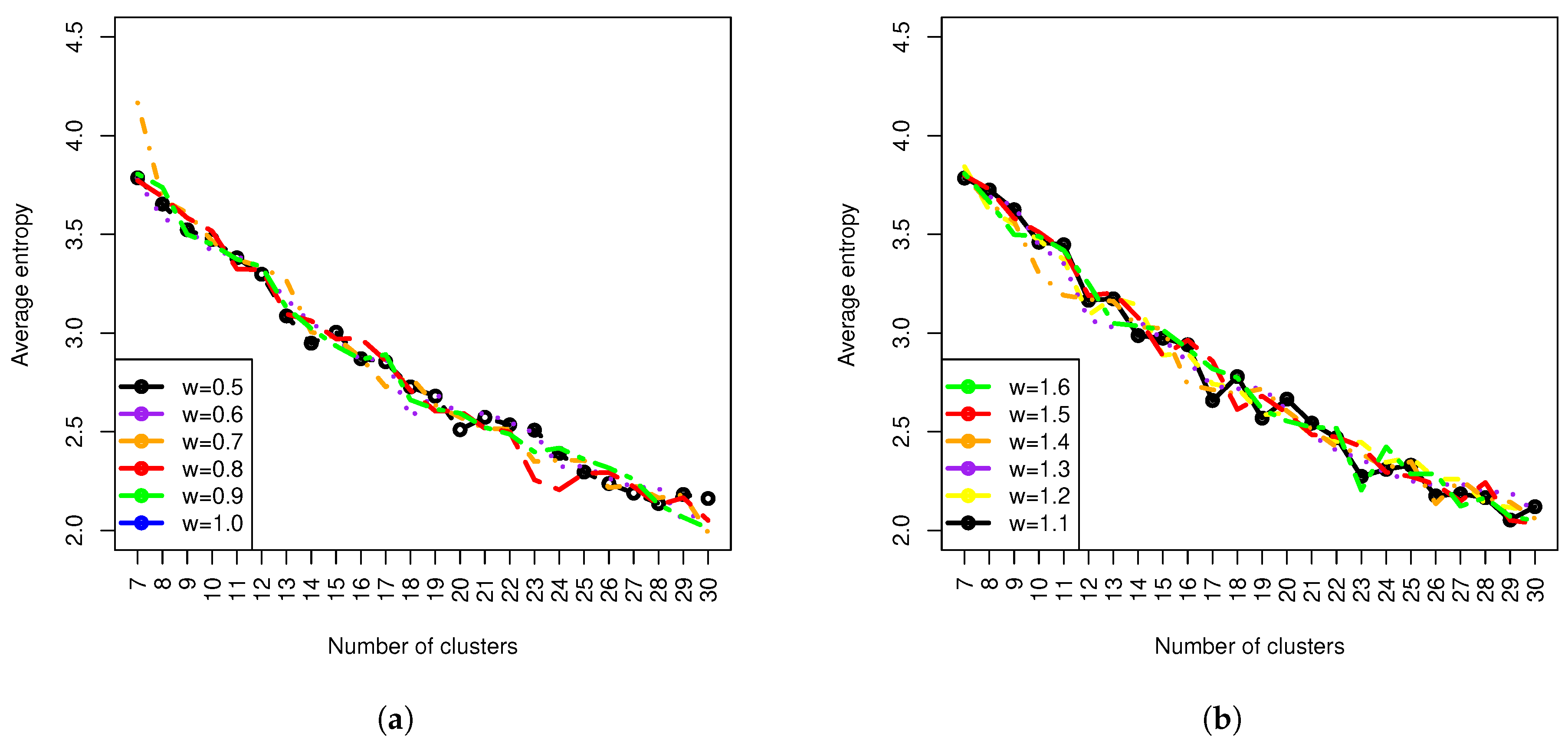
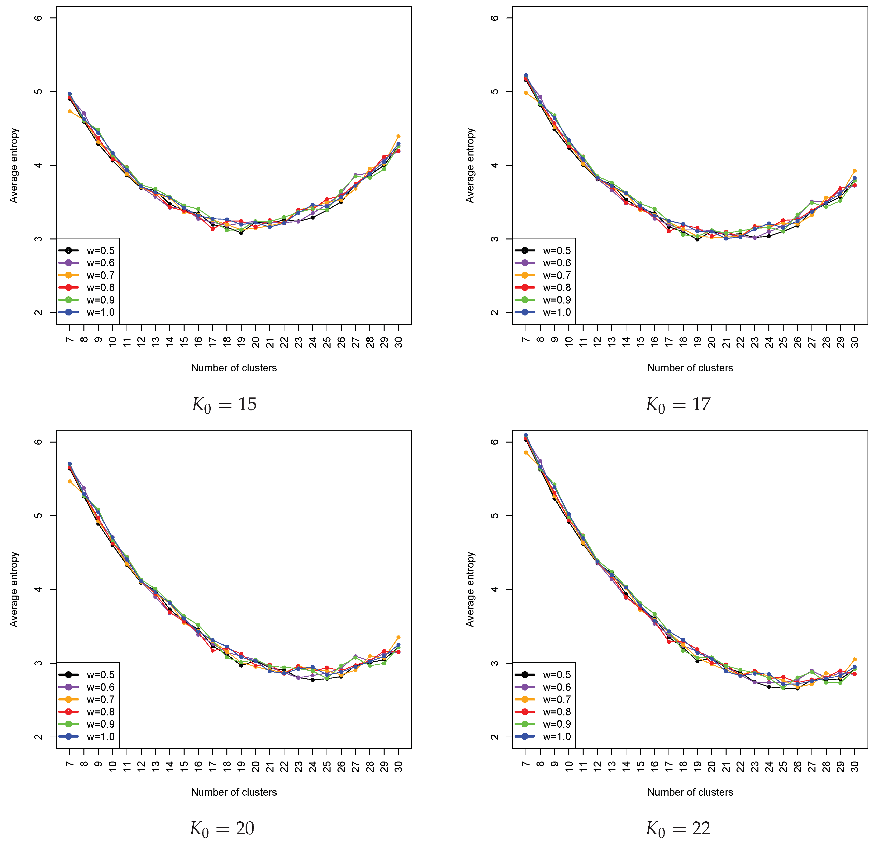
In this paper, the homogeneity of clusters is also assessed using entropy, which was discussed in the methodologysection. It is easily understood that with an increase in the number of clusters, we can expect the decrease of entropy. The entropy for each clustering is weighted by the number of exposures within a cluster. The obtained results using all loss cost data are shown in Figure 5. We also observed that changing the weight value $w_1$ did not have a significant impact on entropy measures. This seems to be appealing as the overall performance of clustering in terms of homogeneity depends only on the K value. Since entropy is a measure of the homogeneity of clusters after clustering, we can see that an optimal selection of the number of clusters does not necessarily lead to an acceptable homogeneity level of a clustering. This finding is of particular importance and is useful for a practical application. It tells us that there may be a cost associated with the pursuit of statistical soundness. The statistical optimality in the selection of a number of clusters does not necessarily guarantee an acceptable homogeneity of a cluster. In practice, it needs to be balanced by increasing the number of clusters to get a better result on homogeneity. Therefore, the choice of the number of clusters suggested by a statistical measure such as the gap statistic or a statistical procedure provides only a starting point or a benchmark on the selection of a number of clusters. When there is another constraint or consideration on the underlying problem, the actual choice on the number of clusters will lose its optimality from the statistical aspect, but still maintain its optimality overall for the problem with consideration of other constraints such as legal requirements. Based on the results in Figure 5, roughly speaking, the choice of the number of clusters in the final model can be chosen as a value between 22 and 26. However, when the entropy is penalized, it turns out that the optimal choice of K is the one that is slightly bigger than the judgemental selection; for example, from Figure 6, when $K_0$ = 20, the optimal choice of K was 24; when $K_0=22$, the optimal choice of K became 26. These results coincide with the results obtained from the qualitative analysis of the entropy pattern displayed in Figure 5. We also observed that our proposed method had a tendency to push the optimal choice of K in an increasing direction from the selection of $K_0$. This may imply that, when our approach is used, one should select a modest value of the total number of groupings to give room for the proposed method to further determine the final optimal choice based on the penalized entropy. The results that correspond to weight values greater than one were similar to the ones that we presented here. Notice that, based on the choice of $K_0=20$ and the use of penalized averaged weighted entropy, the result suggested that the optimal number of grouping was 24, which is slightly larger than the current number that was determined by the classical approach. This may imply that the obtained clustering result is further refined and achieves better homogeneity (i.e., needs larger K) and credibility (i.e., needs smaller K).

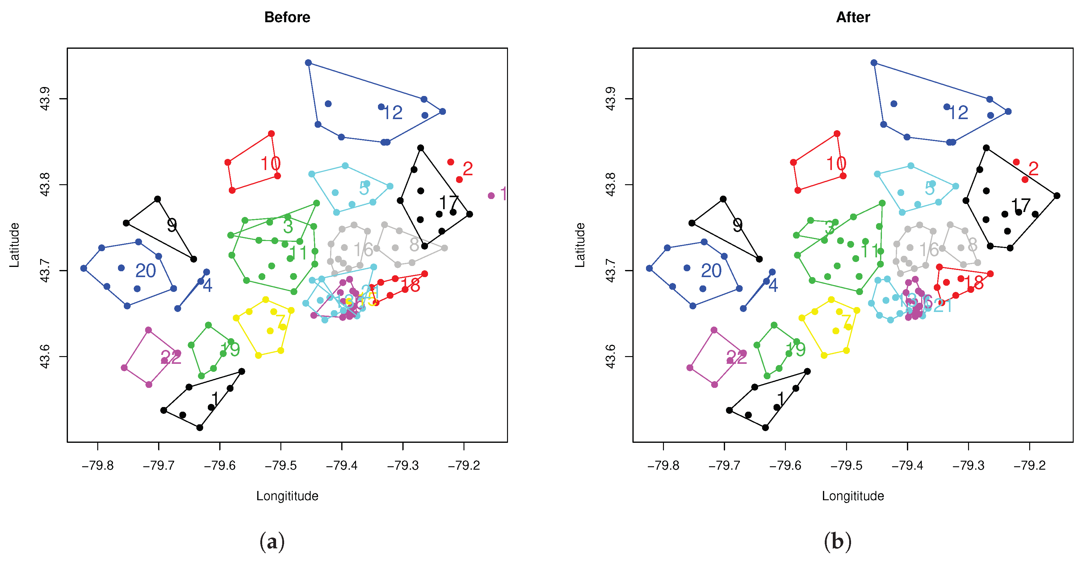
In order to illustrate the improvement of the proposed spatially-constrained clustering, the K-means clustering with $w_1$ = 1 (this implies that geophysical location and loss cost are considered to be equally important) was first applied, and a total of 22 clusters was selected as the number of clusters. The total number of clusters was used by the regulator who owns these data to come up with a design of territory for regulation purposes using the two-step approach discussed in Section 3.5. The choice of 22 clusters was selected for illustration purposes to compare the results before and after using the contiguity constraint. Figure 7a displays the obtained results when K-means clustering was used. From the obtained result, there were still some clusters, such as 3, 13, 15, 21 and 18 (they are indicated within the convex hull plots), that did not completely meet the contiguity requirement. To overcome this issue, the method of using Delaunay triangulation discussed in the methodologysection was applied to further refine the results. The new results are displayed in Figure 7b. From this, we can see that all the clusters formed the convex hull, and the contiguity constraint was satisfied. From the rate regulation perspective, the obtained clusters were further defined as rating territories, and the loss costs were then calculated for each designed territory as a benchmark to ensure that the pricing done by insurance companies is fair and exact. This process will happen in the rate fillings submitted by insurance companies.

5. Concluding Remarks

In rate regulation, it is required that any rate-making methodology being used to analyse insurance loss data must be both statistically and actuarially sound. Ensuring statistical soundness means that the approach being used must convey meaningful statistical information and the obtained results are optimal in the statistical sense. From the actuarial perspective, it requires that any proposed rate-making methodology must take both insurance regulation and actuarial practice into consideration. For example, loss cost must be at a similar level within a given cluster and the total number of territories used for insurance classification should be within a certain range. Furthermore, the number of exposures should be sufficiently large to ensure that the estimate of statistics from the given group is credible. Because of these, it is critical to quantify the clustering effect and balance the results by taking both statistical soundness and actuarial rate and class regulation requirement into consideration.

In this work, spatially-constrained clustering and the entropy method were used to design geographical rating territories using FSA-based loss cost, where FSA was replaced by its geo-coding, which can be easily obtained from some geo-coders. The geo-coding of FSA and their corresponding loss cost were the input of the K-means clustering algorithm. In geo-coding of FSA, the mean value of latitude and the mean value of longitude of all postal codes associated with the same FSA became the coordinates of the centroid of FSA. To ensure the contiguity constraint was satisfied by legal requirements, the method of using Delaunay triangulation was used. A set of real data from a regulator in Canada was used to illustrate the proposed method. The obtained results demonstrated that spatially-constrained clustering is useful for clustering insurance loss cost, which leads to a design of geographical rating territories, which is considered to be both statistically and actuarially sound as the contiguity constraint is satisfied while implementing clustering. Furthermore, the obtained results are able to be further refined by using the penalized entropy method to quantify the homogeneity of groups so that a more suitable number of clusters can be determined. The penalty terms allow us to balance the homogeneity and credibility so that the final optimal selection of the number of groupings is more suitable. The spatially-constrained loss cost clustering is not only important for insurance regulation, where high-level statistics are often needed, but also useful for auto insurance companies in which different rating territories may be required, in order to meet the optimization requirement for the success of business so that the adverse selection may be avoided.