Abstract
Annuities providers become more and more exposed to longevity risk due to the increase in life expectancy. To hedge this risk, new longevity derivatives have been proposed (longevity bonds, q-forwards, S-swaps…). Although academic researchers, policy makers and practitioners have talked about it for years, longevity-linked securities are not widely traded in financial markets, due in particular to the pricing difficulty. In this paper, we compare different existing pricing methods and propose a Cost of Capital approach. Our method is designed to be more consistent with Solvency II requirement (longevity risk assessment is based on a one year time horizon). The price of longevity risk is determined for a S-forward and a S-swap but can be used to price other longevity-linked securities. We also compare this Cost of capital method with some classical pricing approaches. The Hull and White and CIR extended models are used to represent the evolution of mortality over time. We use data for Belgian population to derive prices for the proposed longevity linked securities based on the different methods.
1. Introduction
Significant improvements in longevity have been experienced in most developed countries. For annuity providers, longevity risk, i.e., the risk that future mortality trends differ from those anticipated constitutes an important risk factor.
Under the new European regulatory environment for the insurance industry, Solvency II, it becomes a requirement for insurers to measure and evaluate longevity risks (Levantesi and Menzietti (2006)). As a consequence, the level of the capital required for longevity is increasing ( EIOPA (2011)), and this creates the need for some longevity risk management solutions.
In the past, annuity providers were only able to transfer the longevity risk to reinsurer who can offer a standardized, or a customized hedging with no residual basis risk, but this risk transfer arrangement has become increasingly expensive and present a large counterparty credit risk. In addition, the capacity of reinsurers is limited because longevity risk cannot be diversified, and, as a consequence, just few reinsurers accept taking longevity risk (Blake 2008). Hence, finding other alternatives to transfer the longevity risk, notably securitization, became a necessity (Cox et al. 2013; Li et al. 2019). Another de-risking approach for a pension provider are the pension buy-in and the pension buy-out (D’Amato et al. 2018).
In recent years, some longevity derivatives arose. These products are based on mortality/longevity rates, similar to those existing in the financial market (Blake et al. 2011).
The two main longevity linked securities that were proposed in the literature are longevity bonds (Blake and Burrows 2001), and survival swaps (Dowd et al. 2006).
Longevity swaps are considered better because their transaction costs are lower, are more flexible and could be customized to suit individual circumstances. Moreover, they do not require the existence of a liquid market. Therefore, longevity swaps appear to be the most relevant derivative to consider for hedging longevity risk.
Like the interest rate swaps, the survival swaps can be broken down into a collection of more simple derivative: the Survival-forwards (Coughlan et al. 2007).
These derivatives have attracted many researchers and practitioners who have published many papers on this subject, but because of the pricing difficulties, and the fact that these products remove only the longevity risk, they are still not widely traded in the financial market (Lin et al. 2015).
Some authors have introduced a new methodology inspired by Solvency II: the pricing of longevity derivatives using the Cost of Capital approach. A version of this method has been proposed by (Levantesi and Menzietti 2006) in a discrete time model. In this paper, we generalize this approach in two directions: first, we use a risk measurement more in line with Solvency II and based on successive one-year time horizons; secondly, we model longevity risk with continuous time processes, as they offer analytical tractability and can be used for the pricing of financial instruments. We also study the consistency between this Cost of Capital approach (COC) and three important classical pricing methods used in finance: risk-neutral pricing, Wang transform and Sharpe ratio. This paper is organized as follows: in Section 2, we give the general pricing framework for the S-forward with the classical COC approach, then the same framework is provided in Section 3 for the S-swaps. In Section 4, we translate the theoretical framework into a numerical illustration, enabling the analysis of the consistency between the proposed and the existing classical pricing approaches. We show that none of these methods is completely consistent with the COC approach. Finally, in Section 5, we provide conclusions.
2. Survival-Forwards
As an interest-rate swap is essentially a portfolio of forward-rate agreement (Hull 2009), the survival swap can be broken down into a collection of a more simple derivative: the Survival-forward. Therefore, we will begin our study by focusing on them.
2.1. Definition and Structure
A Survival forward (or S-forward) is an agreement between two counterparties to exchange at a future date T (the maturity of the contract), an amount equal to the realized survival rate of a given population cohort (floating leg), in return for a fixed survival rate agreed at the inception of the contract (fixed rate payment), as shown in Figure 1.

Figure 1.
S-forward.
For easiness of representation, we consider the notional amount equal to one monetary unit. The payoff of the S-forward is then given by:
where is the realized survival rate measurable), and is a fixed probability of an individual aged x at time 0 to be alive at age x + T measurable).
2.2. Assumptions
In order to price the S-forward and S-swap, we will need to make some assumptions. For the whole paper, we will consider the following:
- The longevity is stochastic through one explanatory variable, the mortality intensity denoted by , which represents the force of mortality for an individual aged x + t at time t.
- For this mortality intensity, we consider two affine stochastic time-continuous models (Luciano and Vigna 2015):
- Hull and White model (HW):
- Cox-Ingersoll-Ross (CIR) extended model:
With and all positive numbers, w a standard Brownian motion under the real world probability measure .
The CIR model guarantees the positivity of the force of mortality.
- The spot interest rate is stochastic and is solution of an SDE (Stochastic Differential Equation) of the form:where h and z are two given functions.
- w and are independent standard Brownian motions under the real probability measure .
- We denote by the price at a given time t of an S-forward with maturity T.
- The survival index at time t of an individual initially aged x, alive at time t and surviving T-t years more is given by the following process:
- is the observed survival function measurable).
- The two models being affine, the expectation of their survival index is directly given by (Dowd et al. 2006):
- In the HW model, we have:
- In the CIR extended model, we have:with
- is the price at time t of a zero coupon bound with maturity T under the risk-neutral probability measure .
- There is no basis risk: the insurer’s reference population is the same as in the longevity linked security.
- There is no counterparty default risk.
2.3. S-Forward Pricing by Cost of Capital
There is an ongoing debate and many authors have addressed the question of how to price longevity-linked securities, but the calibration of the market price of longevity risk remains an open question as “ in one hand, there is a quest for actuarial or economic methods of how to derive prices “conceptually” and, on the other hand, there is the problem of how to derive prices given a certain methodology, i.e., what data to use for calibration purposes ” (Bauer et al. 2010).
Some authors have suggested that, following the directive of Solvency II, the price of longevity linked securities could be associated with the Solvency Capital Requirement (SCR) to cover unexpected losses (Börger 2010).
Levantesi and Menzietti (2006) have proposed to price a S-forward using the risk margin implicit within the calculation of the technical provisions as defined by Solvency II.
The overall idea is based on linking the price of longevity-linked securities with the capital that the insurer should hold to cover unexpected losses: according to Solvency II, insurance liabilities that cannot be hedged are evaluated as the sum of a best estimate and a risk margin (RM), which is the market value of the uncertainty on insurance liabilities. The RM is determined by the cost of capital approach based on the SCR, the capital required to cover with 99.5% probability the unexpected losses on a one-year time horizon.
In other words, by entering an S-forward, the insurer can lower its exposition to the longevity risk and, in consequence, the SCR for longevity risk can be mitigated, or even reduced to zero if the longevity risk is completely covered, and so does the corresponding RM. Hence, the price of an S-forward shouldn’t be higher than the cost of holding the SCR; otherwise, insurers won’t be interested in buying it. In fact, this approach provides an estimation of the maximum price that the insurer would be willing to pay to transfer longevity risk.
Let’s consider a T-years S-forward contract (Figure 2).

Figure 2.
T-years S-forward contract.
Under this approach, the price of the S-forward at time t is given by:
where is the best estimate, equal to the discounted expectation of the payoff of the S-forward at time t under the real-world measure, and the risk margin.
At time 0, we obtain:
where is as follows:
The risk margin is defined as the present value of future returns on the successive SCRs:
where is the solvency capital Requirement to cover with 99.5% probability the unexpected losses for year i, and C is the Cost of Capital rate (6% in Solvency II).
These future are random variables. In order to compute the initial risk margin , we need to use their estimation at time 0 denoted by:
The risk margin at time 0 becomes then:
In order to determine the price of an S-forward, we will need to calculate the estimation the future solvency capitals. Solvency II provides different methods to calculate these capitals. We will consider the (Value at Risk) method, which measures the potential loss in value of a risky asset or liability over a defined time horizon for a given confidence level, say 99.5% (Solvency II standard).
2.3.1. Levantesi and Menzietti’s Specification
A first approach developed by (Levantesi and Menzietti 2006) is based on the VaR of the payoff at 99.5% from the moment of calculation until maturity, as represented by Figure 3:

Figure 3.
Computation of the successive in the Levantesi and Menzietti’s specification.
Explicitly, the are given by:
From expression (18), we can see that the Value at Risk is measured on the whole interval [i, T].
The price of the S-forward is then equal to:
2.3.2. Our Specification
To be more consistent with the logic of Solvency II, we propose to adopt another formulation: the SCR at time i should cover with 99.5% probability the unexpected losses on a one-year time horizon (the interval [i, i + 1]), and we consider mortality evolution’s up to time i, and from i + 1 to T according to their best estimates (Figure 4):

Figure 4.
Computation of the successive at time 0 in our specification.
Then, the expression of the becomes:
where
In addition,
The is then given by:
Therefore, the estimation of can be given by:
The risk margin at time 0 is then equal to:
Finally, the price of the S-forward with the COC approach is:
Let us apply these methods in two particular mortality models.
HW Model
In order to determine the explicit expression of the price, we need to compute:
In general, we have:
We know that:
One can show that, under the real-world risk measure , we have:
Thus, the survival index I is log-normally distributed with:
Then, we have:
where is the quantile of a normal distribution N(0, 1).
We consider (Solvency II standard). Finally, the price of the S-forward at time 0 becomes:
with and are given by Equation (7).
CIR Model
Let us here consider that the intensity of mortality follows the CIR process. The same as in the HW model, we will need to determine , but as it is not easy to find an analytical solution, we will simulate it in Section 4. The price of the S-swap is then given by:
where and are given by Equation (8).
2.3.3. Pricing at Any Time t
Following our same reasoning, we give the expression of at any time t (0 < t < i) under the COC approach (Figure 5):

Figure 5.
Computation of the successive at any time t in our specification.
HW Model
We determine under our philosophy the price of an S-forward at time t (0 < t < T) using the Hull and White model:
CIR Model
Let us here consider that the intensity of mortality follows a CIR process. The price of the S-forward at time t becomes:
2.4. Comparison with Classical Methods
We develop in this section the pricing of the S-forward contract, following other alternative theoretical formulas to compare with formula (34):
- The risk-neutral approach (Cairns et al. 2006a),
- The Wang transform (Wang 2002),
- Sharpe ratio (Milevsky et al. 2005).
Numerical comparisons will be given in Section 4.
2.4.1. Risk-Neutral Approach
The risk-neutral pricing is a technique widely used in quantitative finance to compute the values of derivatives, and could be adapted to price longevity-linked securities.
As discussed in some papers, (see for example (Cairns et al. 2006b)), this approach is not ideal to price longevity derivatives as the longevity market is immature, and this method requires the availability of a considered amount of data. However, it is interesting to explore the risk-neutral pricing formula for comparison purpose.
Under the risk-neutral probability measure , the price of an S-forward at time t is given by:
where is the market price of longevity risk.
We first consider the HW model to get an explicit expression of the S-forward price. We assume that follows the HW process given by (2).
Let’s introduce the market prices associated with longevity risk, and let .
We consider a model with a constant market price of risk
The SDE of the force of mortality under the risk-neutral measure becomes:
From Equation (38), we see that a positive value of would increase the drift of the force of mortality. To follow the same insurer’s logic, by overestimating the survival process expected value and underestimating the mortality, we have to choose a negative value for .
Under the risk-neutral measure, the survival probability takes the form:
where and are given by:
Hence, the price of the S-forward at time t with the risk-neutral approach is as follows:
CIR Model
Let us now assume that follows the CIR process given by (3).
We introduce the market prices associated with longevity risk,
Under the real-world probability measure is a Brownian motion with drift, and therefore is not a martingale. According to Girsanov’s theorem, is a standard Brownian motion under the risk-neutral measure .
The SDE of the force of mortality becomes:
The survival probability also takes the form:
We assume that the market price of longevity risk has the following classical form: with is a constant.
Equation (42) then becomes:
The parameters and are given by:
with .
Finally, the price is given by:
2.4.2. Wang Transform Approach
The Wang transform method is a distortion approach that is based on a distortion operator (Leung et al. 2018). In the insurance context, this operator converts the best estimate of the survival index into its risk equivalent using a specific price of risk. This procedure was presented by (Dowd et al. 2006) as a pricing method used in the pricing of several over-the-counter longevity swaps in practice, and used for instance by (Denuit et al. 2007).
The Wang distortion risk measure is given by:
where x is a continuous non-negative random variable.
is its decumulative function, and is the distortion function assiciated with the distortion parameter and given by:
where is the cumulative standard normal distribution
Then:
The price of the S-forward at time t is then given by:
HW Model
To obtain an explicit expression of the S-forward price with the HW model, we need to determine the formula of .
The Wang distortion of a log-normal distribution is still log-normal with a corrected drift parameter:
Thus:
The price of S-forward with Wang approach at time t is finally given by:
CIR Model
Because of its complicated distribution, it is not easy to find an explicit formula for . Hence, we will need an SDE discretization scheme.
For the CIR model, the Euler discretization scheme is as follows:
In order to simulate the survival index , we will make a classical assumption often encountered in life insurance theory: we will suppose that the force of mortality is piecewise constant between each point computed by the above Euler discretization.
We will use an R numerical simulation to determine the price of the S-forward; the algorithm will be described in Section 4.
2.4.3. The Sharpe Ratio Approach
The Sharpe ratio method was used for instance by (Milevsky et al. 2005) and by (Loeys et al. 2007) to price q-forwards. It is a standard deviation principle that does not use a transformation of survival probabilities.
In liquid financial markets, the Sharpe ratio provides a benchmark for the determination of risk premia. The Sharpe ratio is given by:
where is the expected return of the portfolio, is the risk free rate and is the standard deviation of the portfolio return.
Using the analogy to the Sharpe ratio in financial market, the Sharpe ratio in the insurance context (Barrieu and Veraart 2014) is equal to the excess payoff on the longevity-linked securities over its best estimate divided by its standard deviation:
According to this approach, the price of the S-forward is given by:
where S is the chosen fixed Sharpe ratio, and is the variance of the survival index.
HW Model
The variance of the survival process is as follows:
Then:
The price of the S-forward at time t is then given by:
CIR Model
We have:
where:
and:
and are then given by:
with
and can be solved numerically. The variance of the survival index under the real world probability is:
Finally, the price of the S-forward is as follows:
3. Survival-Swaps
As we mentioned previously, the S-swap is considered as the sum of S-forward contracts.
3.1. Definition and Structure
A Survival swap (or S-swap) is a collection of S-forwards exchanged at a predetermined calendar times . Schematically, an S-swap can be represented as follows (Figure 6):
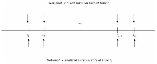
Figure 6.
S-swap structure.
3.2. S-Swap Pricing under the Cost of Capital Approach
Let denote the price of an S-swap at time s (with ). Under the assumption of non-existence of arbitrage opportunities, the price at time s of an S-Swap with as exchange dates is given by:
where is the S-forward price in an approach and a model that have to be specified.
Let us consider an S-swap with n cash flows. The price at time s of an S-swap is given by:
where and are as follows:
We finally find the price of the S-swap at time s:
HW Model
If we consider that the force of mortality follows the HW process, the price under the Cost of Capital approach is given by:
CIR Model
If we consider that the force of mortality follows the CIR process, the price under the Cost of Capital approach is given by:
4. Numerical Illustration
In this section, we give the numerical results of the prices of different S-forwards, using the approaches studied previously for the Belgian population.
We use the following assumptions:
- An insurer with a portfolio of pure endowment contracts paying a lump sum of 1 € at maturity T, and who is interested in hedging its longevity risk.
- initial policyholders for each cohort
- Individuals aged 65, 70, or 75 years old in 2015
- Payment of 1 € to each policyholder alive at time T
- Calibration and fixed leg based on projected data from the IABE unisex projected generational mortality table1.
- The riskless interest rate is constant (equals to 1%).
The fixed rates used for different ages and maturities are reported in Table 1:

Table 1.
The fixed survival rates for different ages and maturities.
4.1. Calibration
We calibrate our models to the data, using the Least Square Estimation method.
HW Model
In order to determine the parameters of the survival function, we calibrate the HW model on projected mortality data for each cohort as explained in the beginning of this section.
The optimal parameters are given by Table 2:

Table 2.
Optimal parameters values for the survival function in the HW model.
CIR Model
The optimal parameters for the three generations are summarized in Table 3:

Table 3.
Optimal parameters values for the survival function in the CIR model.
4.2. S-Forwards COC Prices
Table 4 gives the the prices found under the COC approach, using HW and CIR models for mortality, the different values of the best estimates (BE), and the Risk Margins (RM):

Table 4.
Comparison between the prices of the different S-forwards with HW and CIR models.
In order to have a better idea of the magnitude of these S-forward prices, we can link them with the original price of the pure endowment contract received by the insurer.
The premium P of this pure endowment contract is given by: , with i the technical interest rate.
Table 5 reports a comparison between the premium P and the price of the S forward , considering a technical rate of 0.5% and using COC approach for both models of longevity. is the the hedging cost by

Table 5.
Comparison between the prices of the pure endowment and S-forward contracts.
We can see that is around 1%.
4.3. Consistency with Other Pricing Methods
In this section, we compare numerically the COC approach with other methods developed in Section 2.4. In order to check the consistency between COC and each of these methods, we compute the value of the parameters of the three methods; these parameters are computed such that the COC price is equal to the price given by the considered methods. We can say that a method is consistent with the COC approach if its parameters are quiet stable for different ages and maturities.
4.3.1. Risk Neutral Approach
In this method, we determine the market price of longevity risk, generating the same price as the one found with the COC method.
HW Model
Under the risk-neutral method, and under the assumptions considered previously, the price at time 0 is:
The market price of risk is determined such that this risk-neutral price is equal to the cost of capital price. If this coefficient is stable, it means that the two methods are consistent. Table 6 gives the values of when we use the HW model for longevity:

Table 6.
Equivalent market price of longevity risk in the risk-neutral approach, HW model.
CIR Model
Under the risk-neutral approach, and considering that the intensity of mortality follows the CIR model, the price of the S-forward is:
Table 7 represents the different values of the market price of longevity risk.

Table 7.
Equivalent market price of longevity risk in the risk-neutral approach, CIR model.
Clearly, the two methods are not completely consistent, even if the parameters seem to be more stable in the CIR model.
4.3.2. Consistency with Sharpe Ratio
We will now compute the value of the Sharpe ratio corresponding to the S-forward price found with the COC method.
HW Model
The price with this approach using HW model is given by:
Table 8 gives the equivalent Sharpe ratio generating the prices found with the COC approach.

Table 8.
Equivalent Sharpe parameters, HW model.
CIR Model
With the CIR model, the price of the S-forward at time 0 is given by:
Table 9 presents the different values of the Sharpe parameter under the CIR model:

Table 9.
Equivalent Sharpe parameters, CIR model.
We can see that, for both mortality models, Sharpe parameters have a better stability.
4.3.3. Consistency with Wang Transform
We will now compute the value of the Wang transform parameter corresponding to the COC S-forward price.
HW Model
Table 10 gives the different values of the Wang parameter under the CIR model:

Table 10.
Equivalent Wang parameters, HW model.
CIR Model
For the CIR model, we use numerical simulation to compute the the Wang Transform parameters corresponding to the COC prices. We get the following results:
Table 11 gives the different values of the Wang parameter under the CIR model:

Table 11.
Equivalent Wang parameters, CIR model.
4.3.4. Synthesis
The Cost of Capital approach is parameterized by one variable: the Cost of Capital rate, which is fixed by regulation (6% in Solvency II nowadays). This legal and unique parameter value can be seen as a benchmark, and allows us to find equivalent values of the parameters in the three other methods. The simulations presented above show that:
- None of the classical pricing methods is completely consistent with the COC approach, which is not surprising (the COC price (Formula (26)) is based on a multiperiod formula).
- Sharpe ratio and Wang transform methods seem closer to COC than risk-neutral approach.
- The absolute values found for Sharpe and Wang methods are quite similar. In Appendix A, we present for the HW model complete results for ages between 55 and 85, and maturities from T = 1 to T = 15.
4.3.5. Remark: Smoothing
Taking into account the irregular form of all these prices due to the use of gross mortality parameters for each age (Formulas (2) and (3)), we can smooth these parameters. Appendix B gives the methods used for this smoothing. Appendix B gives then the smoothed prices with COC method in the HW model.
5. Conclusions
In this paper, we have developed in continuous time a new way to price longevity linked securities based on the Cost of Capital approach, consistent with the directive of Solvency II. We considered two examples of stochastic time continuous processes for longevity: Hull and White and CIR extended. This COC method has been compared with three classical methods used in finance: the risk-neutral, Wang and Sharpe methods. More precisely, we have found the parameters of these three methods giving equivalent prices to the COC approach with 6% COC charge, as mentioned in the Solvency II regulation. Even if none of these methods is consistent with the COC approach, it appears that Wang transform and Sharpe ratio methods are more similar to COC than the risk-neutral method. In this paper, we didn’t take into account the basis risk. We could use this proposed COC method to price other longevity linked securities that take into account this risk—for instance, the exchange forwards and exchanged options.
Author Contributions
The two authors have equally contributed to the paper.
Funding
This research received no external funding.
Conflicts of Interest
The authors declare no conflict of interest.
Appendix A
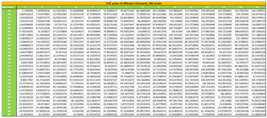
Figure A1.
Prices of S-forward prices under the Cost of Capital approach, HW model.
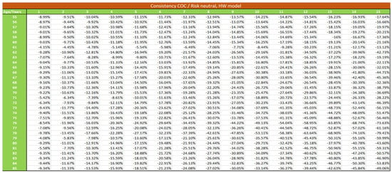
Figure A2.
Consistency between risk-neutral and Cost of Capital method, HW model.
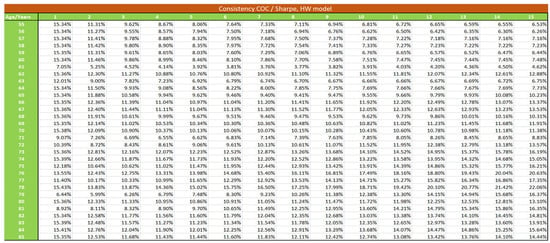
Figure A3.
Consistency between Sharpe and Cost of Capital method, HW model.
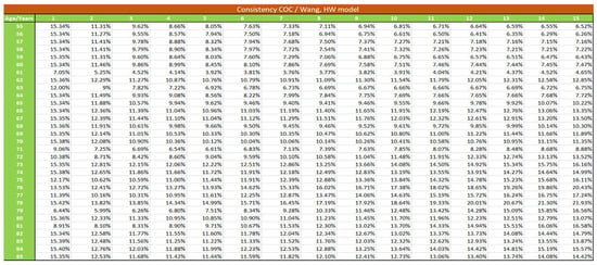
Figure A4.
Consistency between Sharpe and Cost of Capital method, HW model.
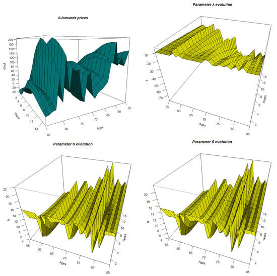
Figure A5.
3D presentation of the S-forwards prices and the corresponding parameters with the other methods.
Appendix B

Table A1.
Nonlinear regression results, HW model.
Table A1.
Nonlinear regression results, HW model.
| Parameter | Fitted Model | Error | Pseudo- |
|---|---|---|---|
| A | 0.004228 | 0.9300884 | |
| a = 2.675 × 10 | |||
| b = −8.947 × 10 | |||
| c = 7.481 × 10 | |||
| B | 0.001877 | 0.5578862 | |
| a = 1.968 × 10 | |||
| b = 2.872 × 10 | |||
| c = −2.154 × 10 | |||
| b | 0.1431 | 0.5408143 | |
| a = 1.968 × 10 | |||
| 0.02138 | 0.1448673 | ||
| a = 0.0002570 | |||
| b = −0.0560466 |
Appendix C
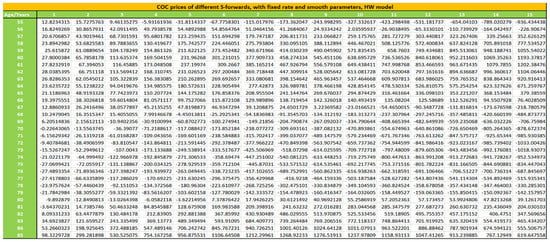
Figure A6.
Prices of S-forward prices under the Cost of Capital approach with smooth parameters, HW model.
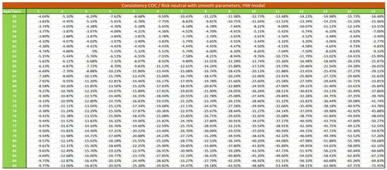
Figure A7.
Consistency between risk neutral and Cost of Capital method with smooth parameters, HW model.
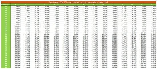
Figure A8.
Consistency between Sharpe and Cost of Capital method with smooth parameters, HW model.
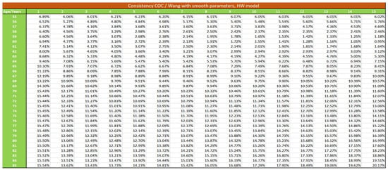
Figure A9.
Consistency between Wang and Cost of Capital method with smooth parameters, HW model.
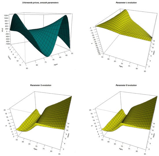
Figure A10.
3D presentation of the S-forwards prices and the corresponding parameters with the other methods.
References
- Barrieu, Pauline, and Luitgard A. M. Veraart. 2014. Pricing q-forward contracts: An evaluation of estimation window and pricing method under different mortality models. Scandinavian Actuarial Journal 2: 1–21. [Google Scholar] [CrossRef][Green Version]
- Bauer Daniel, Matthias Börger, and Jochen Ruß. 2010. On the pricing of longevity-linked securities. Insurance: Mathematics and Economics 46: 139–49. [Google Scholar]
- Blake, David. 2008. Survivor Products: Managing Longevity Risk & Mortality Improvements. Pensions Institute. Available online: http://siteresources.worldbank.org//INTLACREGTOPFINSECDEV/Resources/SurvivorProductsBlake.ppt (accessed on 15 March 2018).
- Blake, David, Andrew J. G. Cairns, and Kevin Dowd. 2011. Living with Mortality: Longevity Bonds and Other Mortality-Linked Securities. British Actuarial Journal 12: 135–97. [Google Scholar] [CrossRef]
- Blake, David, and William Burrows. 2001. Survivor bonds: Helping to hedge mortality. Journal of Risk and Insurance 68: 339–48. [Google Scholar] [CrossRef]
- Börger, Matthias. 2010. Deterministic shock vs. stochastic value at risk: An analysis of the Solvency 2 standard model approach to longevity risk. Blätter DGVFM 31: 225–59. [Google Scholar] [CrossRef]
- Cairns, Andrew J. G., David Blake, and Kevin Dowd. 2006a. A two-factor model for stochastic mortality with parameter uncertainty: Theory and calibration. Journal of Risk and Insurance 73: 687–718. [Google Scholar] [CrossRef]
- Cairns, Andrew J. G., David Blake, and Kevin Dowd. 2006b. Pricing deaths: Frameworks for the valuation and securitisation of mortality risk. ASTIN Bulletin 36: 79–120. [Google Scholar] [CrossRef]
- Coughlan, Guy, David Epstein, Amit Sinha, and Paul Honig. 2007. Q-Forwards: Derivatives for Transferring Longevity and Mortality Risks. New York: JP Morgan Pension Advisory Group. [Google Scholar]
- Cox, Samuel H., Yijia Lin, Ruilin Tian, and Jifeng Yu. 2013. Managing Capital Market and Longevity Risks in a Defined Benefit Pension Plan. Journal of Risk and Insurance 3: 585–619. [Google Scholar] [CrossRef]
- D’Amato, Valeria, Emilia Di Lorenzo, Steven Haberman, Pretty Sagoo, and Marilena Sibillo. 2018. De-risking strategy: Longevity spread buy-in. Insurance: Mathematics and Economics 79: 124–36. [Google Scholar] [CrossRef]
- Denuit, Michel, Pierre Devolder, and Anne-Cécile Goderniaux. 2007. Securitization of Longevity Risk: Pricing Survivor Bonds with Wang Transform in the Lee-Carter Framework. Journal of Risk & Insurance 74: 87–113. [Google Scholar]
- Dowd, Kevin, David Blake, Andrew J. G. Cairns, and Paul Dawson. 2006. Survivor swaps. Journal of Risk and Insurance 73: 1–17. [Google Scholar] [CrossRef]
- EIOPA. 2011. EIOPA Report on the Fifth Quantitative Impact Study (QIS5) for Solvency II. EIOPA-TFQIS5-11/001. Frankfurt: EIOPA. [Google Scholar]
- Hull, John C. 2009. Options, Futures, and Other Derivatives, 3rd ed. Upper Saddle River: Pearson Prentice Hall. [Google Scholar]
- Leung, Melvern, Man Chung Fung, and Colin O’Hare. 2018. A comparative study of pricing approaches for longevity instruments. Insurance: Mathematics and Economics 82: 95–116. [Google Scholar] [CrossRef]
- Levantesi, Susanna, and Massimiliano Menzietti. 2006. Maximum Market Price of Longevity Risk under Solvency Regimes: The Case of Solvency II. Risks 5: 29. [Google Scholar] [CrossRef]
- Li, Jackie, Chong It Tan, Sixian Tang, and Jia Liu. 2019. On the optimal hedge ratio in index-based longevity risk hedging. European Actuarial Journal, 1–17. [Google Scholar] [CrossRef]
- Lin, YiJia, Richard D. MacMinn, and Ruilin Tian. 2015. De-risking defined benefit plans. Insurance: Mathematics and Economics 63: 52–65. [Google Scholar] [CrossRef]
- Loeys, Jan, Nikolaos Panigirtzoglou, and Ruy M. Ribeiro. 2007. Longevity: A Market in the Making. New York: J.P. Morgan Securities Ltd. [Google Scholar]
- Luciano, Elisa, and Elena Vigna. 2015. Non mean reverting affine processes for stochastic mortality. ICER Working Papers. Available online: https://pdfs.semanticscholar.org/078c/db5b0e614b28bbb68ee899e046d0fb8339c2.pdf (accessed on 24 February 2018).
- Milevsky, Moshe A., David S. Promislow, and Virginia R. Young. 2005. Financial Valuation of Mortality Risk via the Instantaneous Sharpe Ratio: Application to Pricing Pure Endowments. Working Paper. Ann Arbor: University of Michigan. [Google Scholar]
- Wang, Shaun S. 2002. A Universal Framework for Pricing Financial and Insurance Risks. Astin Bulletin 32: 213–34. [Google Scholar] [CrossRef]
| 1 | IA|BE Mortality projection for the Belgian population, 2015. Available from: https://www.iabe.be/nl/iabe-mortality-tables. |
© 2019 by the authors. Licensee MDPI, Basel, Switzerland. This article is an open access article distributed under the terms and conditions of the Creative Commons Attribution (CC BY) license (http://creativecommons.org/licenses/by/4.0/).