Figure 1.
First trips of drivers 57 (left), 206 (middle) and 238 (right): the lower line in blue color shows the speeds (in km/h), the upper line in red color shows that acceleration/braking (in m/s), and the middle line in black color shows the changes in angle .
Figure 1.
First trips of drivers 57 (left), 206 (middle) and 238 (right): the lower line in blue color shows the speeds (in km/h), the upper line in red color shows that acceleration/braking (in m/s), and the middle line in black color shows the changes in angle .
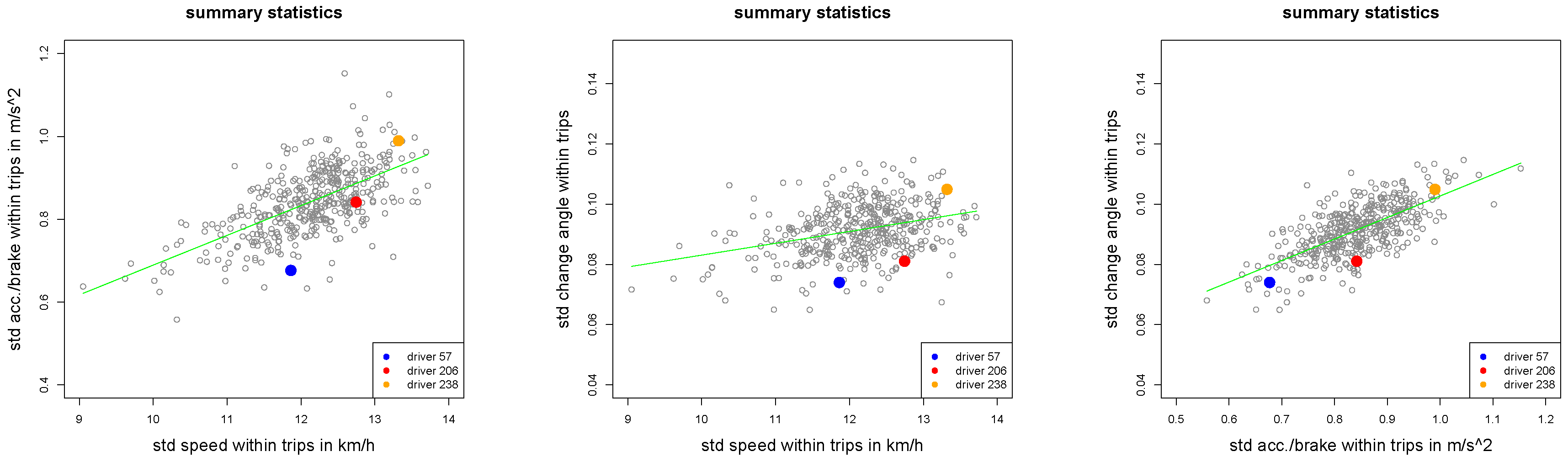
Figure 2.
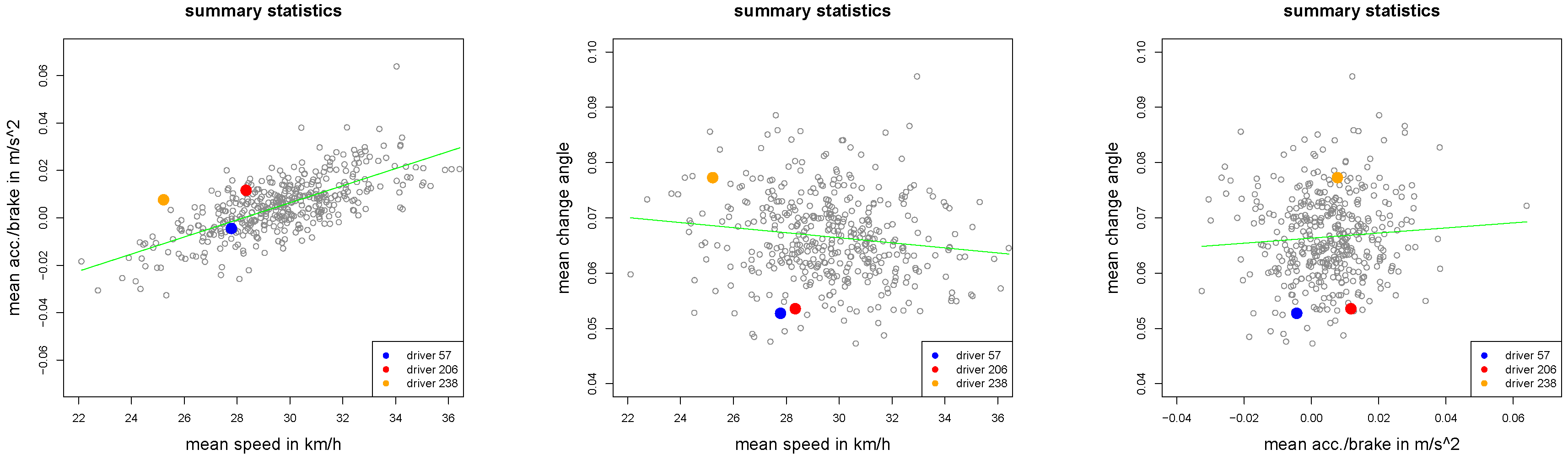
Summary statistics , and of all drivers.
Figure 2.
Summary statistics , and of all drivers.
Figure 3.
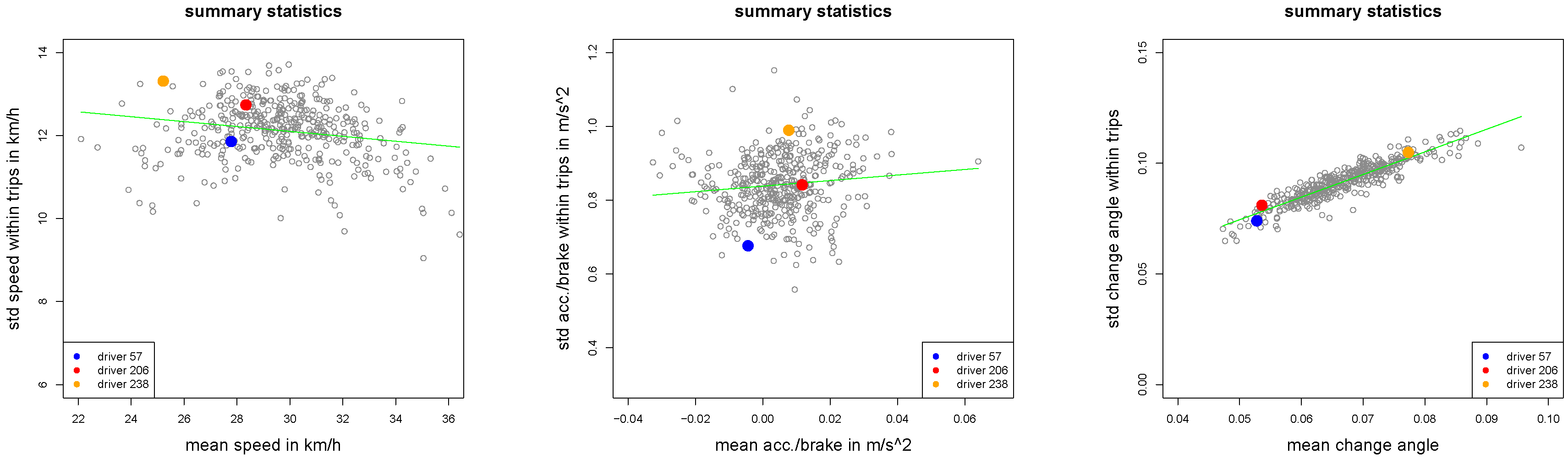
Empirical standard deviations (
2) plotted against empirical means (
1) for all
drivers.
Figure 3.
Empirical standard deviations (
2) plotted against empirical means (
1) for all
drivers.
Figure 4.
Summary statistics , and of all drivers.
Figure 4.
Summary statistics , and of all drivers.
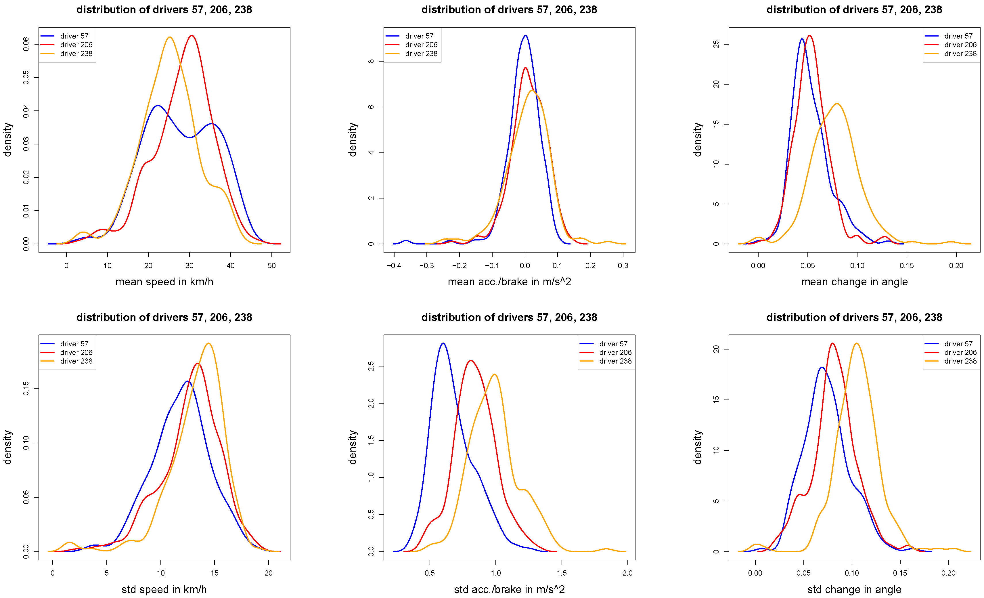
Figure 5.
Densities of the individual trip statistics , and (first row), and , and (second row) for of the three selected drivers 57, 206 and 238.
Figure 5.
Densities of the individual trip statistics , and (first row), and , and (second row) for of the three selected drivers 57, 206 and 238.
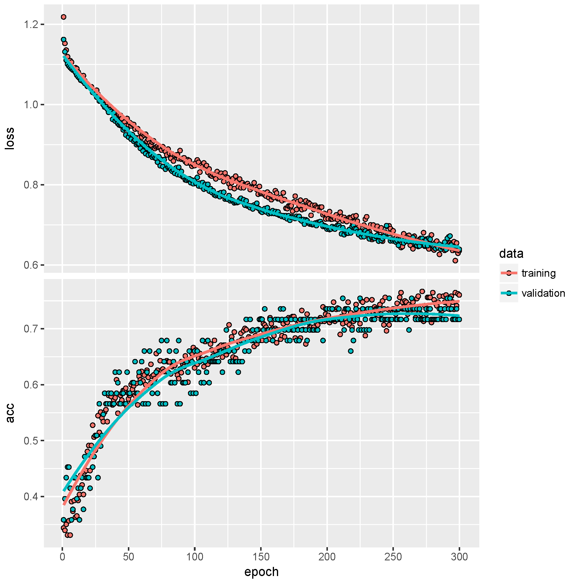
Figure 6.
Stochastic gradient descent fitting of the ConvNet given in
Listing 2 to the individual trips of the drivers 57, 206 and 238: the upper graph shows the categorical cross-entropy losses; the lower graph shows the correct classification rates for training (red) and validation (blue) data.
Figure 6.
Stochastic gradient descent fitting of the ConvNet given in
Listing 2 to the individual trips of the drivers 57, 206 and 238: the upper graph shows the categorical cross-entropy losses; the lower graph shows the correct classification rates for training (red) and validation (blue) data.
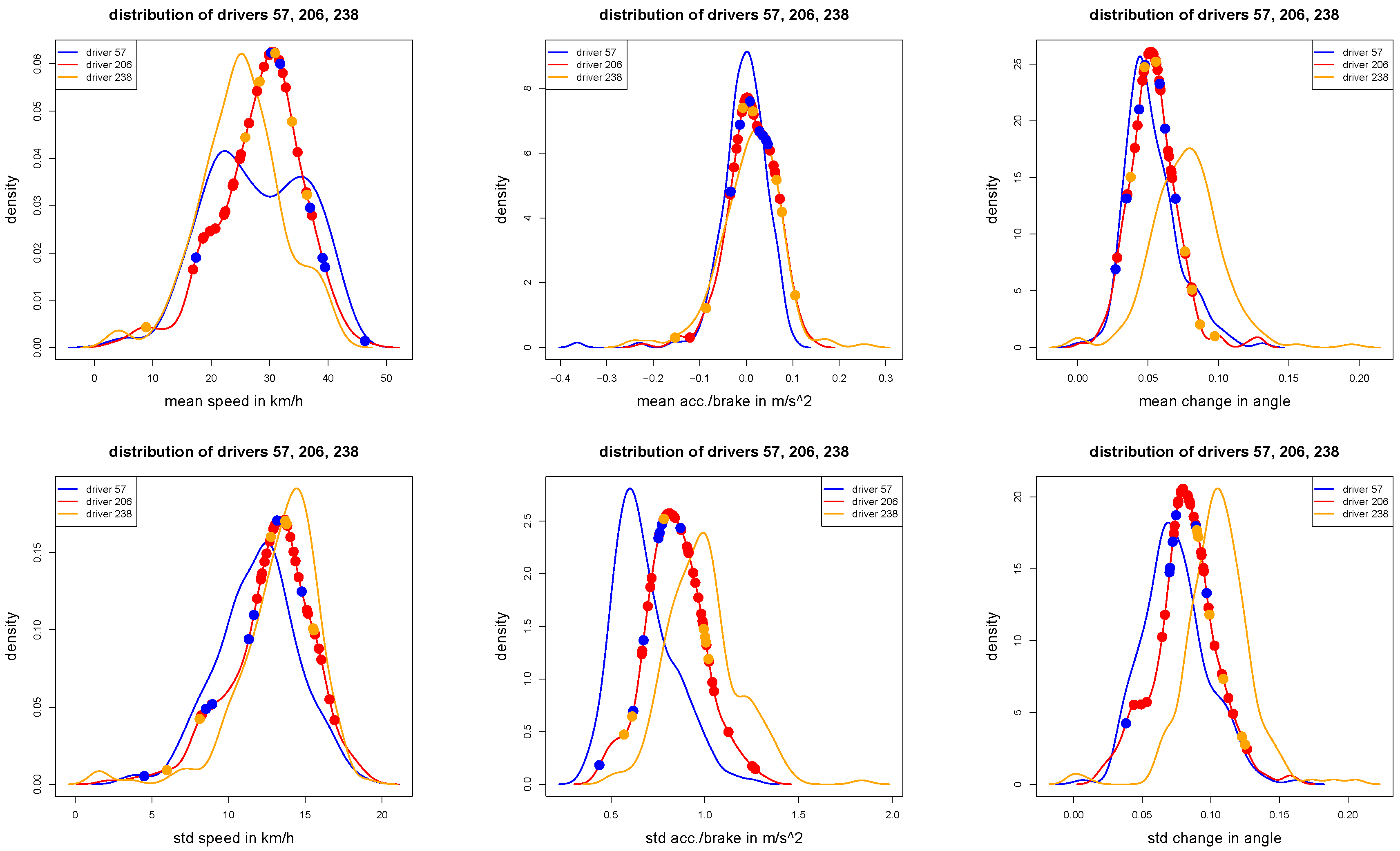
Figure 7.
These figures show the same densities as in
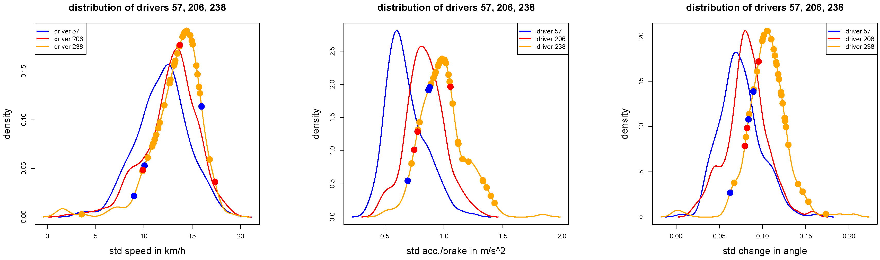
Figure 5: the dots illustrate the 47 test samples of driver 206: red dots show correctly classified trips, blue and orange dots show misclassified trips (according to the given wrong labels).
Figure 7.
These figures show the same densities as in
Figure 5: the dots illustrate the 47 test samples of driver 206: red dots show correctly classified trips, blue and orange dots show misclassified trips (according to the given wrong labels).
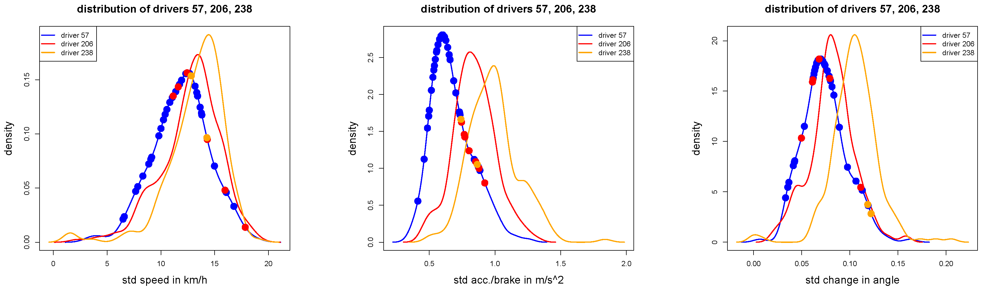
Figure 8.
Out-of-sample analysis of the 42 test samples of driver 57: correctly classified trips (blue dots) and misclassified trips (red and orange dots according to the given labels) of driver 57, illustrated in the density plots of , and for .
Figure 8.
Out-of-sample analysis of the 42 test samples of driver 57: correctly classified trips (blue dots) and misclassified trips (red and orange dots according to the given labels) of driver 57, illustrated in the density plots of , and for .
Figure 9.
Out-of-sample analysis of the 42 test samples of driver 238: correctly classified trips (orange dots) and misclassified trips (blue and red dots according to the given labels) of driver 238, illustrated in the density plots of , and for .
Figure 9.
Out-of-sample analysis of the 42 test samples of driver 238: correctly classified trips (orange dots) and misclassified trips (blue and red dots according to the given labels) of driver 238, illustrated in the density plots of , and for .
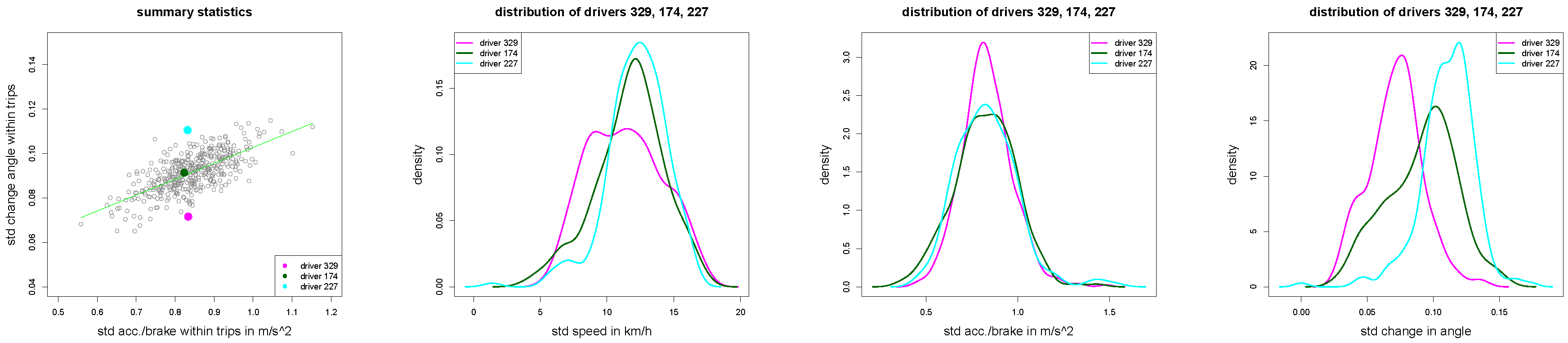
Figure 10.
(left) Scatter plot of all drivers with drivers 329, 174 and 227 in magenta, green and cyan colors; (middle and right) density plots of , and for of the three drivers 329, 174 and 227.
Figure 10.
(left) Scatter plot of all drivers with drivers 329, 174 and 227 in magenta, green and cyan colors; (middle and right) density plots of , and for of the three drivers 329, 174 and 227.
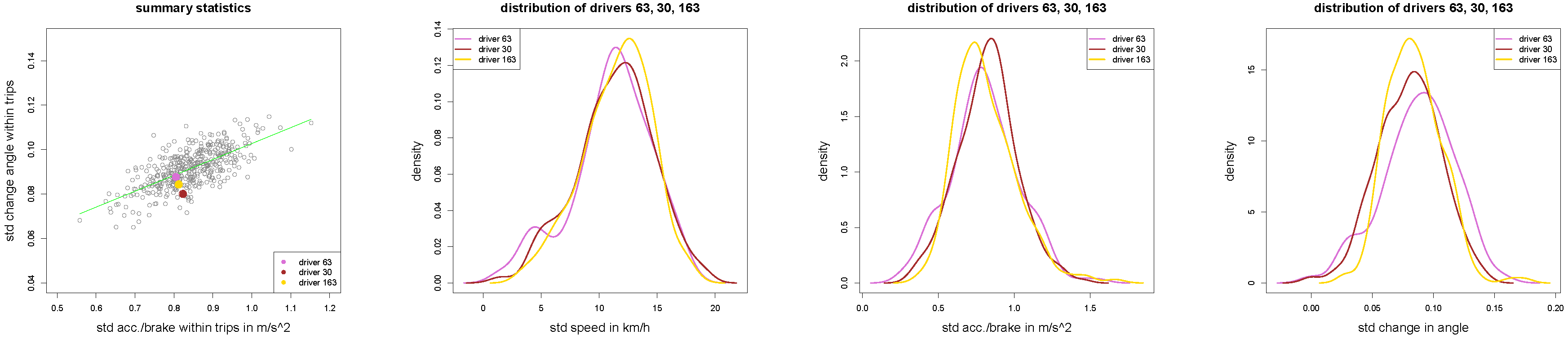
Figure 11.
(left) Scatter plot of all drivers with drivers 63, 30 and 163 in orchid, brown and yellow colors; (middle and right) density plots of , and for of the three drivers 63, 30 and 163.
Figure 11.
(left) Scatter plot of all drivers with drivers 63, 30 and 163 in orchid, brown and yellow colors; (middle and right) density plots of , and for of the three drivers 63, 30 and 163.
Figure 12.
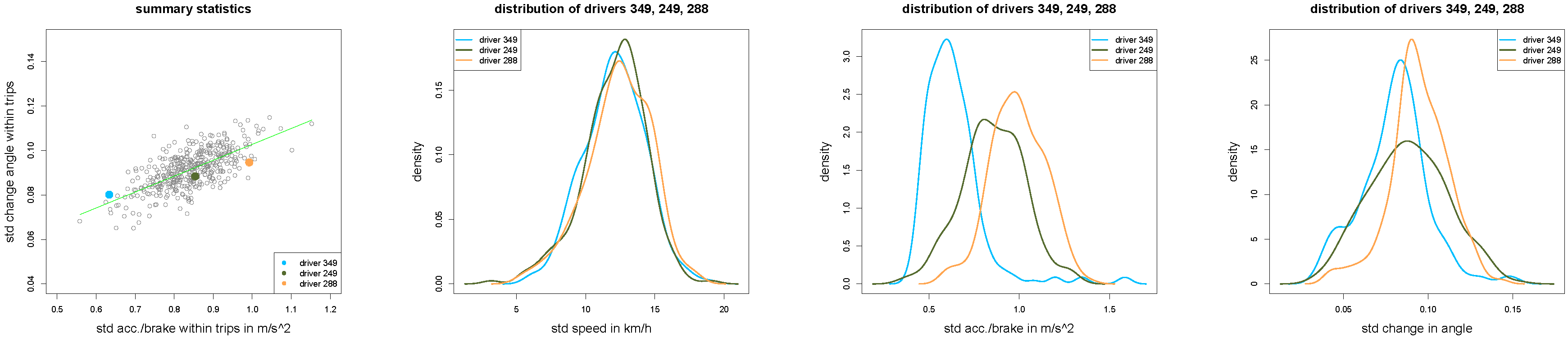
(left) Scatter plot of all drivers with drivers 349, 249 and 288 in light blue, dark green and orange colors; (middle and right) density plots of , and for of the three drivers 349, 249 and 288.
Figure 12.
(left) Scatter plot of all drivers with drivers 349, 249 and 288 in light blue, dark green and orange colors; (middle and right) density plots of , and for of the three drivers 349, 249 and 288.
Figure 13.
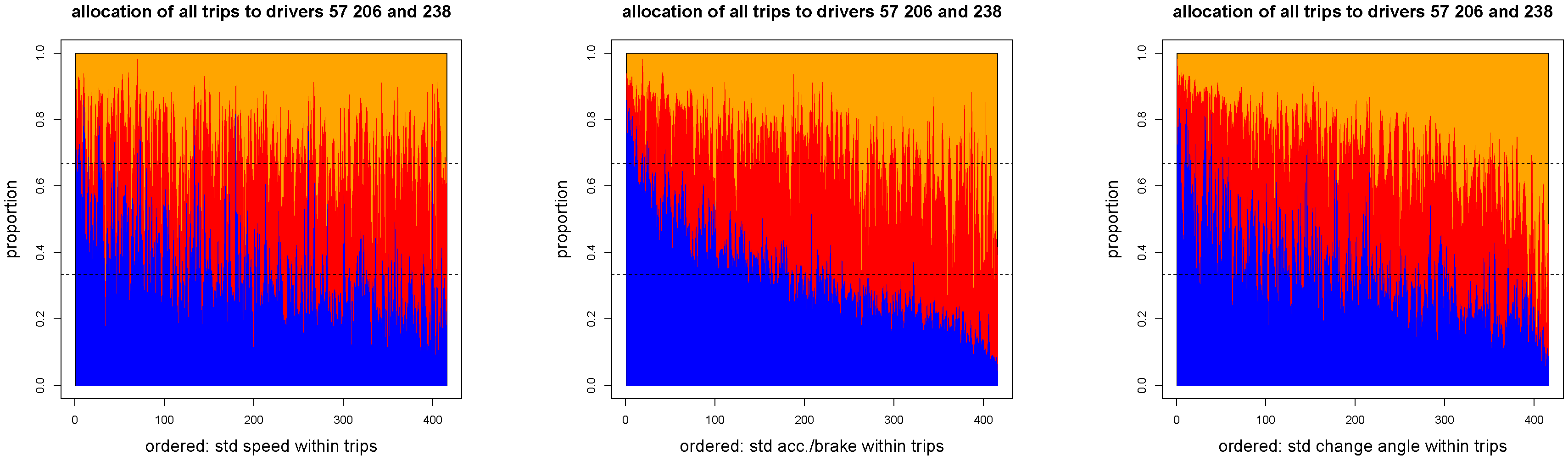
Relative allocation of the individual trips of drivers to drivers 57 (blue), 206 (red) and 238 (orange): individual drivers are ordered w.r.t. (left), (middle) and (right).
Figure 13.
Relative allocation of the individual trips of drivers to drivers 57 (blue), 206 (red) and 238 (orange): individual drivers are ordered w.r.t. (left), (middle) and (right).
Figure 14.
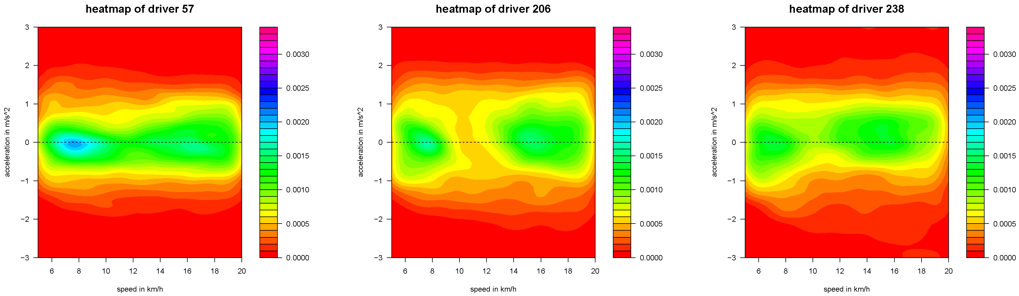
v-a heatmaps of the three selected drivers .
Figure 14.
v-a heatmaps of the three selected drivers .
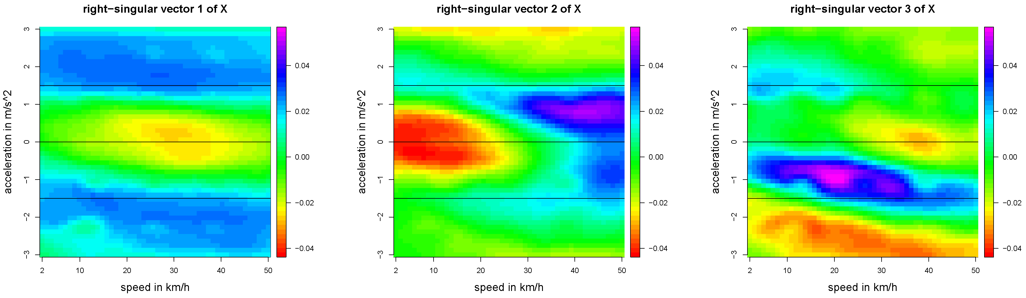
Figure 15.
First three right-singular vectors of X given by the first three columns of the orthogonal matrix V.
Figure 15.
First three right-singular vectors of X given by the first three columns of the orthogonal matrix V.
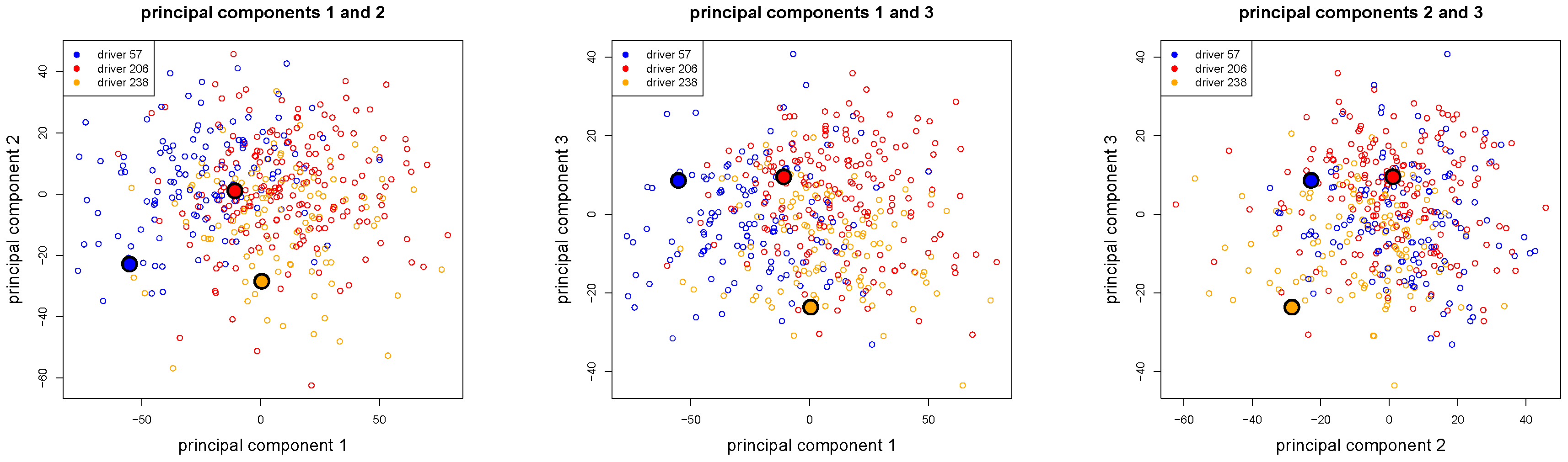
Figure 16.
The first three principal components of the
drivers illustrated in two-dimensional scatter plots, colored according to the ConvNet classification of
Table 6, the three selected drivers 57, 206 and 238 are illustrated by bigger dots.
Figure 16.
The first three principal components of the
drivers illustrated in two-dimensional scatter plots, colored according to the ConvNet classification of
Table 6, the three selected drivers 57, 206 and 238 are illustrated by bigger dots.
Table 1.
Out-of-sample analysis of drivers 57, 206 and 238.
Table 1.
Out-of-sample analysis of drivers 57, 206 and 238.
| Variable | Driver 57 | Driver 206 | Driver 238 |
|---|
| Total number of trips S | 205 | 234 | 213 |
| Size learning sample | 163 | 187 | 171 |
| Size test sample | 42 | 47 | 42 |
| Correctly classified test samples (in %) | 78.6% | 70.2% | 85.7% |
| Misclassified test samples | 9 | 14 | 6 |
Table 2.
Confusion matrix of the out-of-sample analysis of
Table 1.
Table 2.
Confusion matrix of the out-of-sample analysis of
Table 1.
| | True Labels |
|---|
| | Driver 57 | Driver 206 | Driver 238 |
|---|
| Predicted label 57 | 33 | 7 | 3 |
| Predicted label 206 | 7 | 33 | 3 |
| Predicted label 238 | 2 | 7 | 36 |
Table 3.
Out-of-sample analysis of drivers 329, 174 and 227.
Table 3.
Out-of-sample analysis of drivers 329, 174 and 227.
| Variable | Driver 329 | Driver 174 | Driver 227 |
|---|
| Total number of trips S | 446 | 232 | 214 |
| Size learning sample | 356 | 186 | 171 |
| Size test sample | 90 | 46 | 43 |
| Correctly classified test samples (in %) | 86.7% | 54.3% | 76.7% |
| Misclassified test samples | 12 | 21 | 10 |
Table 4.
Out-of-sample analysis of drivers 63, 30 and 163.
Table 4.
Out-of-sample analysis of drivers 63, 30 and 163.
| Variable | Driver 63 | Driver 30 | Driver 163 |
|---|
| Total number of trips S | 194 | 259 | 203 |
| Size learning sample | 155 | 207 | 163 |
| Size test sample | 39 | 52 | 40 |
| Correctly classified test samples (in %) | 35.9% | 59.6% | 45.0% |
| Misclassified test samples | 25 | 21 | 22 |
Table 5.
Out-of-sample analysis of drivers 249, 349 and 288.
Table 5.
Out-of-sample analysis of drivers 249, 349 and 288.
| Variable | Driver 349 | Driver 249 | Driver 288 |
|---|
| Total number of trips S | 244 | 255 | 193 |
| Size learning sample | 195 | 203 | 155 |
| Size test sample | 49 | 52 | 38 |
| Correctly classified test samples (in %) | 83.7% | 67.3% | 78.9% |
| Misclassified test samples | 8 | 17 | 8 |
Table 6.
Allocation of all trips to the three drivers 57, 206 and 238, and allocation of the drivers to the three selected drivers according to the likelihood of the individual trip allocation.
Table 6.
Allocation of all trips to the three drivers 57, 206 and 238, and allocation of the drivers to the three selected drivers according to the likelihood of the individual trip allocation.
| Variable | Driver 57 | Driver 206 | Driver 238 |
|---|
| Allocation of all 103,734 trips | 35.0% | 35.2% | 29.7% |
| Allocation of the 416 drivers | 29.8% | 45.0% | 25.2% |


