1. Introduction
The seminal work by
Markowitz (
1952) initiated modern portfolio theory and provided a solution to the portfolio selection problem according to a mean-variance criterion. The mean-variance optimal portfolio is the one that maximizes its expected return at a given level of risk, measured by its variance, or conversely the one that minimizes its risk at a given level of expected return. This one period model has known multiple extensions, among them the discrete time multi-period model by
Samuelson (
1969) and the continuous time model by
Merton (
1969).
Initially, the parameters of these models have been considered known and constant, especially the parameters that drive the behavior of the assets: drifts and covariances. It not only oversimplifies the reality but also it raises the question of estimating these parameters. The most basic and widely used method consists of estimating drifts and covariances from past data and fix them once and for all. Estimating volatility in this way appears to give relatively good results in practice, while estimating the drift seems to be more difficult or even impossible, see
Merton (
1980). Moreover, optimal portfolios are very sensitive to the level of expected returns, as shown in
Best and Grauer (
1991), and a wrong estimation can result in very suboptimal portfolios a posteriori. See also
Elliott et al. (
1998) and
Siegel and Woodgate (
2007) for more details about these issues.
This explains the development of the literature on parameters uncertainty in portfolio analysis, see for instance
Barry (
1974) and
Klein and Bawa (
1976), and especially on Bayesian statistics, see (
Aguilar and West 2000;
Avramov and Zhou 2010;
Bodnar et al. 2017;
Frost and Savarino 1986). Nonetheless, these models remain static and cannot benefit from the flow of information which results in a nonadaptive strategy, unable to process the most recent information conveyed by the assets market prices. It is one of the main reasons why literature on filtering and learning techniques in a partial information framework has developed, see (
Cvitanić et al. (
2006);
Rogers (
2001);
Lakner 1995,
1998). The Bayesian learning approach consists of modeling the uncertainty of a set of parameters by a prior distribution, representing the beliefs of the investor on the potential values of the parameters, which is updated with incoming information, for instance assets market prices. In particular, in our companion paper
De Franco et al. (
2018), we have solved the multidimensional Markowitz problem in the case of an uncertain drift using Bayesian learning with a Gaussian prior and have provided a brief analysis of sensitivities of the optimal solution w.r.t. the different parameters.
In this paper, we adapt the results in
De Franco et al. (
2018) to implement the strategy in practice. Indeed, the solution provided is in continuous time and the amounts invested in the assets are unconstrained. Of course, in reality, trading is discrete and amounts invested in assets are limited, so we discretize the optimal solution of the continuous Markowitz problem, turn amounts into proportions and cap the optimal proportions to be invested in order to fit the portfolio management constraints. Our purpose is to show the prevalence of the Bayesian learning strategy above the nonlearning one which considers the drift constant. To do so, we illustrate our point by confronting both strategies to different datasets representing different investment universes. First, we use a panel of major indices in four different asset classes: corporate bonds, sovereign bonds, commodities and equities completed with cash. Then, we consider bank accounts in foreign banks that pay the local interest rate but are valued in EUR, in order to study the performance of both strategies with respect to foreign exchange rates. Finally, we implement both strategies in an investment universe composed of smart beta strategies. Moreover, using the first dataset, we provide a sensitivity analysis of both strategies to various parameters: the uncertainty in the model, the impact of the leverage, the review frequency and the rebalancing frequency. We do not show this analysis for the two other datasets since we would find similar results.
The paper is organized as follows.
Section 2 details the model and the discretized optimal strategies while
Section 3 depicts the market data and the workflow.
Section 4 shows the results in the case of the first dataset, and
Section 5 is about the sensitivity analysis of the Bayesian learning and the nonlearning strategies applied to this dataset. Finally,
Section 6 deals with foreign exchange rates and
Section 7 with smart beta strategies.
2. The Framework
We consider a financial market consisting of one risk-free asset, whose return is denoted by
, and
n risky assets whose returns
are modeled by
We shall assume that the random vectors
are independent for all
t. Model (
1) includes major linear models available in the financial literature, such as CAPM (
Lintner 1965;
Sharpe 1964), discrete-time Black-Scholes (
Black and Scholes 1973) or Fama-French models (
Fama and French 1993,
2015,
2016).
is the vector of the expected returns of the risky assets, while
is the covariance matrix of the risky assets. We assume that
exists. We denote by
the set of admissible investment strategies. An admissible strategy
represents the fraction of wealth invested in the assets at any time
t. Recalling from the self-financing condition that,
we write the wealth at maturity
as
We consider an investor who is aiming to solve the Markowitz problem:
where
is the risk tolerance for the investor.
The initial version of the Markowitz problem (
Markowitz 1952), which was stated for a single period, has been widely studied and solutions in the multi-period framework (such ours) in both discrete and continuous time have been provided (see e.g.,
Karatzas et al. (
1987);
Merton 1969,
1975;
Samuelson (
1969) among others). The common assumptions in previous works are that both expected return and volatility coefficients (
and
in our framework) are known. In practice, these parameters are not directly observable and must be estimated from the data or input by the investor at inception. In both cases, biased parameters can significantly affect ex-post performance of the optimal strategy. Although the parameter
can be estimated from the data with some degree of confidence, the estimation of
turns out to be quite difficult, if not impossible. Because the optimal strategy strongly depends on both
and
, a wrong estimation could significantly affect the optimal strategy.
To get closer to reality and account for model uncertainty, we assume reasonably that the investor has an a priori view on the risky assets and their expected returns, but she is uncertain about how good her forecast is. Introducing uncertainty into the problem brings it closer to the real-life situation, where not only does the investor not know the parameters of the model, but is also forced to admit that her estimates are uncertain. More precisely, the investor does not observe and only assumes that , where is a probability distribution in centered at . The parameter is the vector of returns the investor is expecting, while translates her uncertainty about it.
Remark 1. When —the Dirac distribution at —the investor has no uncertainty about her forecast.
Remark 2 (Discretization)
. Implementing optimal strategies in practice leads to continuous adjustments to the optimal solutions in time and makes them suboptimal. Here, we discretize the continuous optimal solutions and controls, and cap them. To propose a solution to Problem (2), we suggest confronting the discretized continuous optimal Bayesian learning and nonlearning solutions since the investor can observe assets prices nearly continuously but trades in discrete time.
The paper
De Franco et al. (
2018) solved the continuous-time version of problem (
1) for a large class of distributions
with
in a Bayesian framework using dynamic programming techniques. We report here the discretized version of the results in the Gaussian case
: Let
with
. Then, the discretized version of the continuous-time optimal solution of the Bayesian–Markowitz problem is given by (the Bayesian learning case,
BL)
where
is the wealth process at time
s and
,
is defined as ,
,
R is the unique solution to the following semi-linear parabolic PDE
which in the case of a Gaussian prior proves to be of the form
, where
is the solution to a multidimensional Riccati equation, for which the solution can be found explicitly, and
r is the solution to a first-order linear differential equation depending on
and
, which can also be explicitly calculated. See
De Franco et al. (
2018) for further details.
The process is the conditional expectation of given the current observation of the assets returns, which are given by . The matrix represents the uncertainty around . As time goes by, we observe more returns which in turns improves our knowledge of , as one can see from the fact that when , more weight is put on in the definition of . The matrix valued function is linked to the conditional covariance of given .
Remark 3. When there is no uncertainty (), or when the investor directly inputs her estimate , the structure of the discretized version of the optimal continuous solution is simplified as follows (the nonlearning case, NL
):where ,
.
The main differences between the Bayesian learning and the nonlearning strategies arise from
the market risk premium R in the leverage coefficient,
the correction term which is zero for the nonlearning strategy.
As time goes by, we observe realized returns and we learn more about . Indeed, with uncertainty, the Bayesian learning strategy is updated with , which is the conditional expectation of given the current observation (new knowledge). The trade is modified with the corrective term .
Both and are unconstrained. In order to provide a realistic analysis on both strategies, we consider capped versions of them.
Definition 1. The capping operator for an investment strategy with a leverage iswhere .
In
Section 3, we will implement both the Bayesian learning and the nonlearning strategies in the context of asset allocation with real market data, to get insights on the effect of learning and its value added (
value of information).
3. Market Data
We consider four asset classes across different regions, each of which is represented by a well-known market index detailed in
Table 1, and the EONIA rate as the risk-free rate for an investor whose base currency is the Euro.
Non-Euro-denominated indices are hedged against the Euro simply by implementing a monthly rolled hedging overlay with one-month forward contracts. We collected data from December 1998, except for the EUR Corporate Liquid High Yield for which we only obtained data from January 2006. Prices were sourced from Bloomberg, while currency spot and forward rates came from Datastream and both refer to the 4 p.m. London fixing. Our choice of market indices is motivated by their popularity among investors, their liquidity, and the wide range of financial products available in the market that give exposures to these indices (such as listed futures and ETFs). While limited in number, they provide well-diversified exposures to major global asset classes. Therefore, this suits the underlying premises of the Markowitz problem which is less suited for asset allocation in presence of many underlyings.
The testing period is from January 2000 to June 2018. To implement both
BL and
NL, we iteratively followed the workflow outlined below and
Table 2 collects the parameters (in bold in the workflow) used for our test.
Work Flow 1.
Let and consider the time-frame .
We call a Review date since at this date we estimate all the parameters and calculate the function R that define in (
3)
and in (
4).
To ensure a realistic implementation of both strategies, all data-based estimations are performed with data available before the Review date and ending on . The first Review date is 21 January 2000.
We call a Rebalancing date if, at this date, we updated the portfolio weights according to (
3)
and (
4).
To limit turnover and transaction costs, the subsets of Rebalancing dates in is relatively small. We assume that both Review and Rebalancing dates are Fridays, so that the number of Rebalancing dates in the period is given by the frequency Freq.
is estimated as the sample mean over the pastdays ending onor over the maximum data available with a minimum of 30 data points. is estimated as the sample covariance matrix overdays ending onor over the maximum data available with a minimum of 30 data points.
We consider a parametric function for as follows:
The motivation behind our choice comes from Problem (
2).
Indeed, we expect thatand we set so that within our confidence interval, the gap to the expected value of is a fraction of the initial wealth The uncertainty around the estimate is measured by . We assume to be diagonal. Therefore, each diagonal entry measures the degree of confidence we have on the relative entry of . Each diagonal entry is modeled as follows:
where is the 95% (5%) quantile of the empirical distribution of the return . To calculate these quantiles, we consider the time series of the returns spanning for days and ending on . Up to the parameter , the square root of is half of the segment, centered at the median, that contains 90% of the empirical distribution over days.
Strategies and are considered in their capped versions according to Definition 1 with a maximum leverage.
At time T, we rerun the workflow by setting and update all parameters according to the new data available.
It should be noted that the choice of diagonal does not imply that assets are uncorrelated. The matrix represents the uncertainty the investor has around her initial prior . While assets are correlated, we assume that the investor makes her initial expectations on and she only includes her anticipated error due to uncertainty on her expectations. To simplify, we do not include off-diagonal terms (uncertainty on pairwise cross-expectations), because this allows for a simple, one-parameter modeling of uncertainty in .
Our choice of reflects the assumption that investors anticipate the assets returns to be equal to , and the error, which is unknown and represents their uncertainty around the expectation , depends on the width of the empirical distribution of returns. In practice, if we decide to proxy expected returns with the average of past returns (which of course is known to be a very poor indicator of future returns), then the width of the empirical distribution, here measured by the difference between the 95% and 5% quantiles, serves as a proxy for uncertainty. The fine-tuning parameter is a simple way to increase the uncertainty in the initial guess .
The workflow above and
Table 2 represent the
Base Case. In
Section 4, we report the results for both the Bayesian learning (
BL) and the nonlearning (
NL) strategies over the last 18 years. In
Section 5, we will assess the sensitivity of both strategies to changes in the parameters of the
Base Case to get a better grasp of the value added of learning in the context of portfolio construction.
4. The Base Case Result
We implemented the workflow to build the wealth processes
and
as in (
2) related to the
BL and
NL strategies in the Base Case framework (
Table 2). For the sake of simplicity, we refer to
BL as either the strategy weights
or the associated wealth process
and we do the same for
NL.
Table 3 collects some long term statistics for both strategies. Although our choice of statistics is limited and many other interesting properties could have been easily derived, such as skew, kurtosis, VaR, CVaR or turnover (as e.g., in
Scaillet (
2004)), we prefer to show the statistics that are usually considered at any initial due diligence for investment strategies, such as annualized performance, volatility, maximum drawdown, Sharpe ratios and information ratios. The main reason behind our choice is to provide evidence on the effect of learning in the improvement of long-term performance.
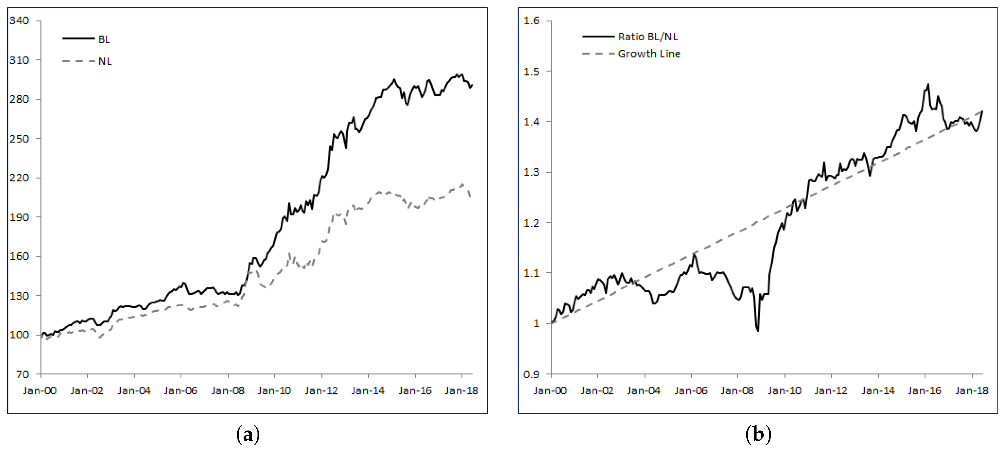
Over the period from January 2000 to June 2018, BL delivered an annualized performance of 5.96% while NL reached 3.96%. Incorporating uncertainty and learning from the data yielded an annualized 2% excess return. In terms of risk metrics, annualized volatility is slightly higher for BL (0.59% difference) but also shows a better maximum drawdown figure (−8.51% for BL versus −11.20% for NL). Finally, the Sharpe ratio is 1.08 for BL versus 0.80 for NL, or a 34.26% improvement in relative terms. The information ratio of BL over NL is about 0.55, meaning that the performance of BL comes from a better ability to process incoming information.
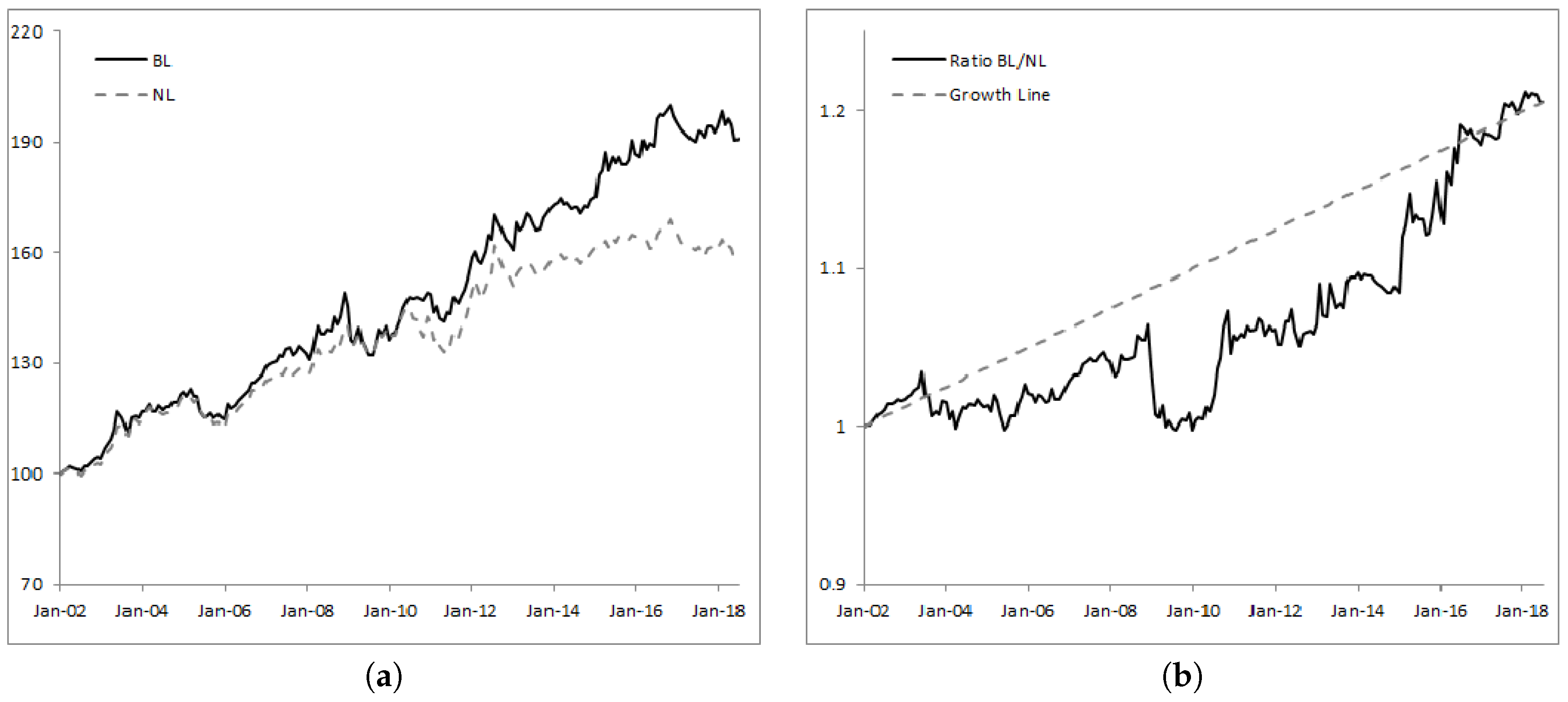
Figure 1a shows the historical levels of the wealth processes
BL and
NL, while
Figure 1b provides the relative strength of
BL over
NL as well as the growth line. An increasing relative strength index signals outperformance of
BL over
NL, while a decreasing index shows underperformance.
Looking at
Figure 1b,
BL mostly delivers a more robust and more regular performance than
NL. Integrating uncertainty in the drift, learning from the data and adjusting the strategy accordingly clearly adds value over time. Specifically, we identify three distinct periods: from inception until February 2006 the ratio
BL/
NL has an upward trend at moderate pace, reaching 1.13 (or equivalently 13% cumulated outperformance); then
BL underperforms
NL until October 2008; and finally, from October 2008 to June 2018,
BL strongly dominates
NL with
of cumulated outperformance.
5. Sensitivity Analysis
In the following paragraphs, we will stress-test the
BL strategy by measuring the effects of the main parameters on long term results. Our stress-test methodology consists in fixing all but one of the parameters detailed in
Table 2 and varying the remaining parameter across plausible values.
5.1. Impact of Uncertainty
Here, we study the effect of the uncertainty parameter
in the strategy. Higher values of
signal a higher volatility of the estimate
, hence a higher uncertainty on the estimate of the expected returns. We study the
BL strategy for
, where the value
corresponds to the Base Case detailed in
Section 4.
Table 4 shows the results.
Intuitively, among the
BL strategies detailed in
Table 4, the strategy with
is the closest to
NL and this is confirmed by the performance and volatility figures. Indeed, with such a low level of uncertainty, we are confident in our initial estimate
. As we increase
, the confidence we place in
decreases.
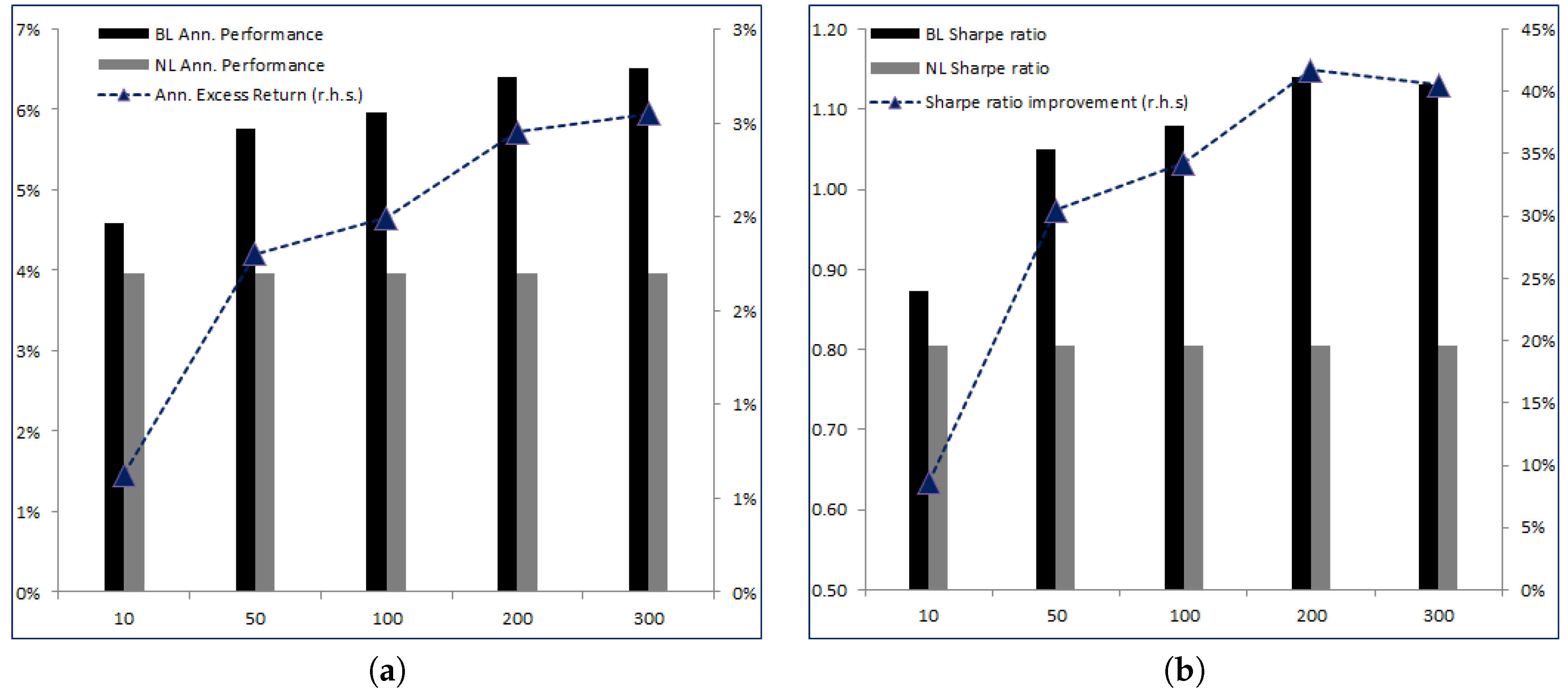
Very interestingly, as increases, the excess return of the corresponding BL strategy over NL increases without significantly increasing the risk. Therefore, Sharpe ratios increase with from 0.87 for to 1.13 for . More striking is the relative increase in Sharpe ratios with respect to NL—for we only have an increase of 8.64% and for the relative increase is 40.54%. Finally, the Information ratio rapidly stabilizes around 0.5.
Figure 2a,b graphically renders the increase in both annualized performances, excess returns and Sharpe ratios with respect to
NL as a function of
.
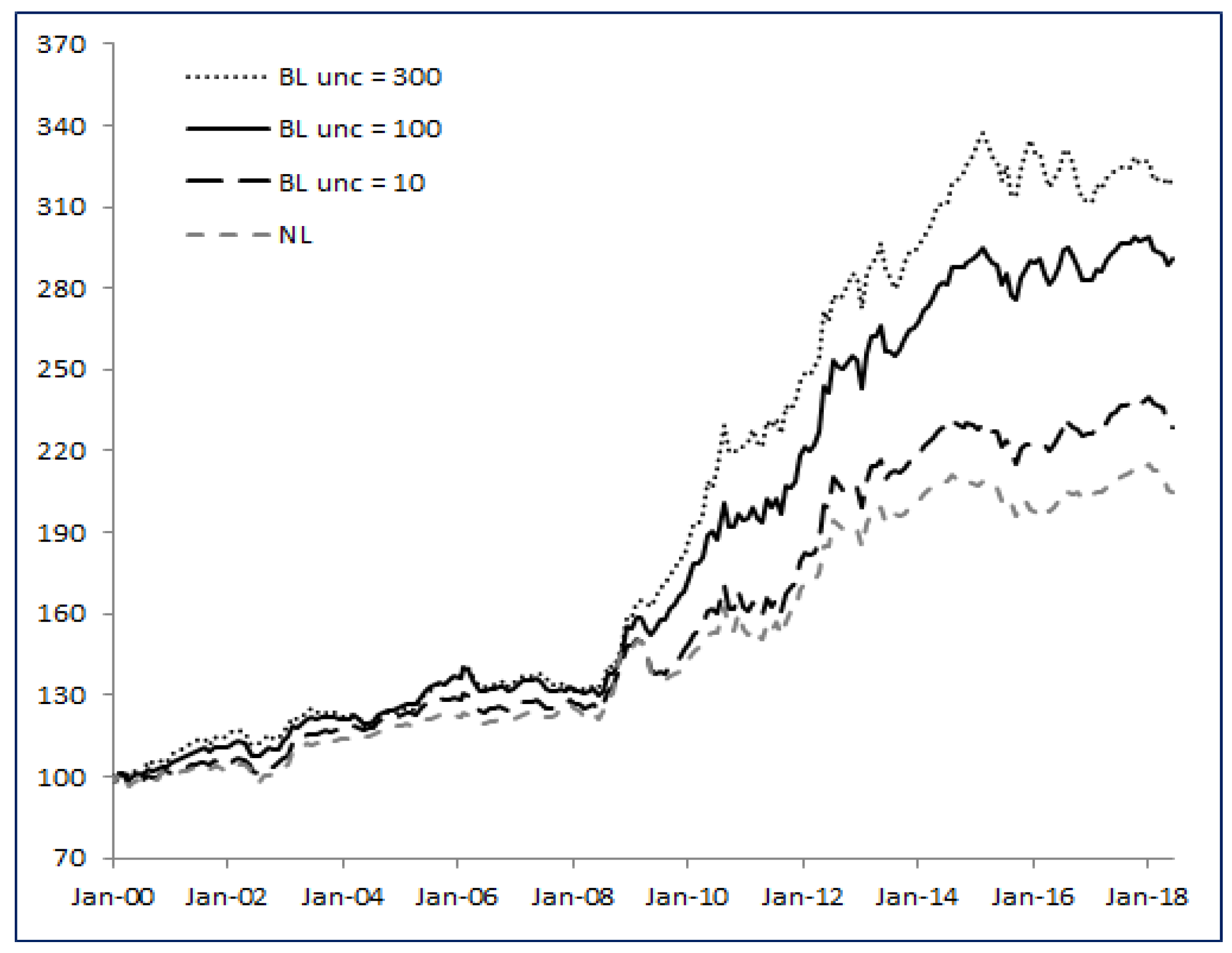
Figure 3 shows the historical levels of the strategy
BL with
(minimum uncertainty),
(high uncertainty) and
(Base Case) compared to
NL. The
BL strategies share the same profile, but the higher the
parameter, the higher the excess return we find in the long run.
Clearly, the standard solution to the Markowitz problem suffers from the poor estimate of , while the BL strategy is able to adjust and react to new observable data. Moreover, the higher the uncertainty, the better BL behaves compared to NL.
Unreported tests showed us that with this particular dataset, we can increase the parameter even further. At some point though, around 10,000, the BL strategy underperforms NL. Indeed, when uncertainty is extremely high, the matrix that controls the a priori knowledge we have on is simply uninformative because we are allowing to span too vast a region of potential values. Therefore, the learning process, over a relatively short period of time of three months, is slow and does not add value.
5.2. Impact of Leverage
We now look at the maximum leverage parameter
L in both strategies. Higher values of
L make both
and
closer to the unconstrained weights. We test
, where the value
corresponds to the Base Case detailed in
Section 4.
Table 5 collects the results, while
Figure 4a,b gives a graphical overview of the impact on long term statistics.
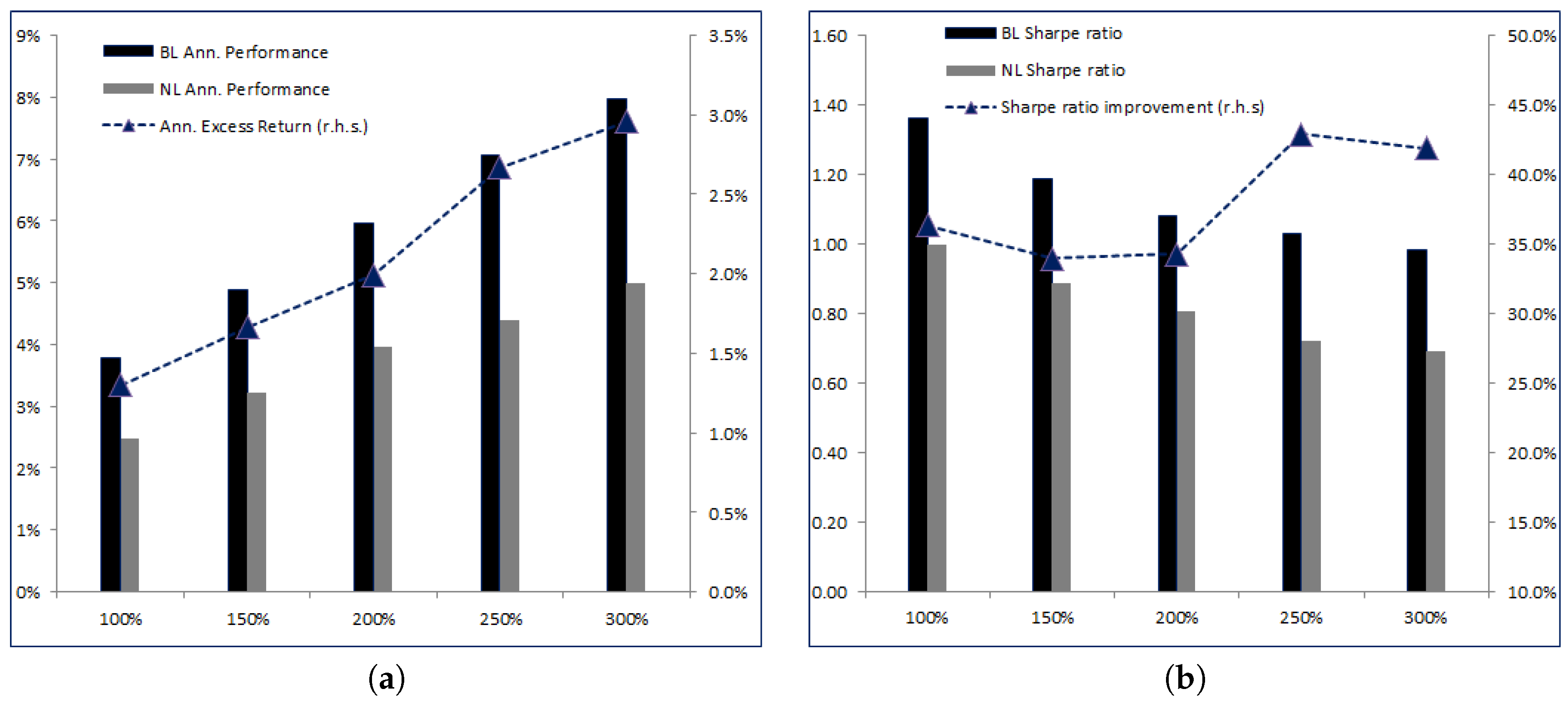
As the maximum leverage L increases, the corresponding excess return of the BL strategy over NL increases. For L = 100%, the excess return is 1.30% and goes up to 2.96% for L = 300%.
Clearly, and as expected, the excess return increases with the leverage and on average we observe that adding 100% of leverage brings 0.80% in extra excess return. When we look at the Sharpe ratios, we see that BL always outperforms NL but the relation is more complex than the previous one. Both BL and NL Sharpe ratios decrease with L. Indeed, as L increases, we observe higher performances but also higher volatilities, and the volatility grows faster than the performance. This is obvious, because when L increases the strategy becomes more sensitive to any error in the estimated parameters, which is reflected in higher volatility. As , the strategies become unconstrained and bring all the instability that is well known to go alongside with price-based strategies. On a relative basis, the improvement in the Sharpe ratios first decreases as L reaches 200% and then increases.
To conclude, it appears that the impact of the maximum leverage
L is as expected—it brings extra performance at the cost of higher risk. Because we know real data do not need to follow model (
1), unconstrained
BL and
NL (as any price-based strategies) tend to amplify any model error, making the leverage constraint a wise feature to consider.
5.3. Impact of the Review Frequency
Probably one of the most important features of the learning effect on the portfolio is the frequency at which we recalibrate the parameters of the model. We have chosen a three-month frequency in the Base Case. In other words, every three months we compute new estimates of
and
and input a new matrix
, driving the uncertainty. We expected that the lower the frequency, the better
BL would compare to
NL. The main reason behind this thesis is that the strategy
NL will be stuck with parameters
and
for a long period of time, during which we know that they will most likely become obsolete as the market evolves and new information is processed. As investors know very well, forecasting is difficult and outdated forecasts are badly suited for portfolio construction
1. On the other side,
BL can adapt over time because it embeds uncertainty about
.
Let us consider the frequency parameter
Freq in both strategies varying from three to twelve months,
, where the value
corresponds to the Base Case detailed in
Section 4.
Table 6 shows the results.
As we lower the review frequency, we see the performances of both
BL and
NL decreasing. Nevertheless, the excess return of
BL over
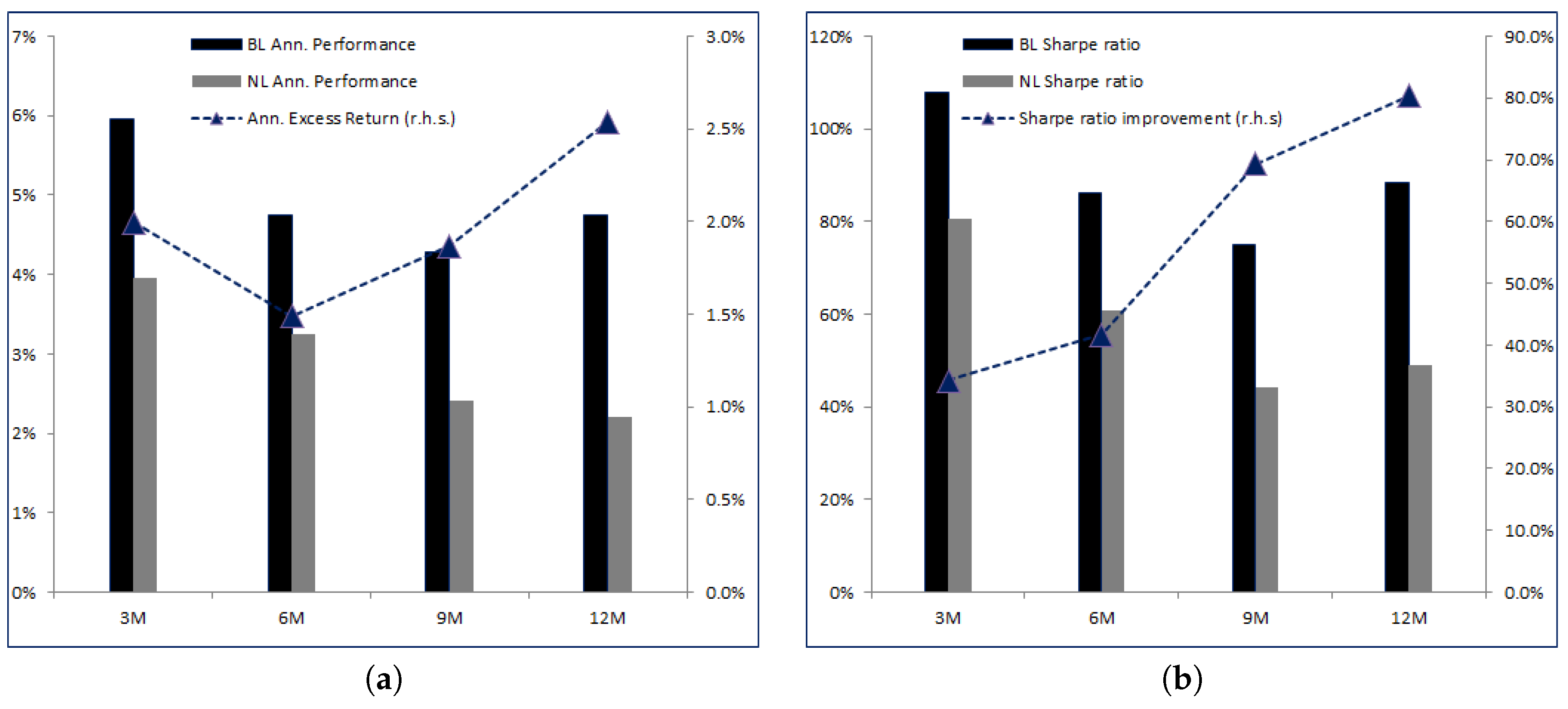
NL actually increases at frequencies lower than 6-month. The fact that it is not monotonic is related to the timing effect. The best metric to assess the value added of the learning feature remains the relative improvement in Sharpe ratios, as shown in
Figure 5b. Here we see that as the frequency lowers, more risk-adjusted value added comes from the learning effect: at 3 months, the relative improvement in Sharpe ratio between
BL and
NL is 34.26%. At 6 months it goes up to 41.47%, then 69.38% at 9 months and finally 80.4% relative improvement at the 12-month frequency. Clearly,
BL outperforms
NL if we do not review the parameters of the model quite often, and this is clearly attributable to the fact that
BL can adjust over time according to the data observed and the adjustments it can make on the a priori distribution of
.
For the sake of simplicity, we do not report the results here, but it is possible to increase the efficiency of
BL compared to
NL if we simultaneously modify the frequency
Freq and the uncertainty parameter
unc in
. Over long investment horizons, the investor would definitely habr more uncertainty on her a priori estimate
, therefore it makes perfect sense to consider
Freq = 12 coupled with
unc = 1600 or higher
2.
5.4. Impact of Rebalancing Frequency
We conclude this section with an overview on the impact of the rebalancing frequency on both
BL and
NL. This exercise is only theoretical, since within the Base Case we only performed three trades (one each month before the next review). A lower rebalancing frequency of trading would mean that we do not fully exploit the power of learning by adjusting the portfolio. Higher rebalancing frequency carries a turnover (and transaction cost) issue, that would make any benefit only hypothetical. Furthermore, when we rebalance too often, we embark significant amount of noise coming from daily, short term, price movements. Usually, practitioners consider higher rebalancing frequencies only for a small portion of the portfolio, i.e., they only rebalance a fraction
x of their portfolio while keeping the remaining
unchanged and they roll over. Because this goes beyond the scope of this paper, we limit ourselves to monthly versus biweekly rebalancing frequency.
Table 7 collects summary statistics for
BL and
NL when the optimal weights in the Base Case are implemented on both monthly and biweekly frequencies.
As we go from the monthly to the biweekly rebalancing frequency, we observe a small decrease in annualized performance of
BL, while the drop is more significant for
NL. Although these numbers should not be taken as very informative due to the timing effect, there is clearly not a strong incentive for
BL to rebalance more often, since performance goes down slightly, as does volatility. In the end, the Sharpe ratio seems fairly stable. On the other hand,
NL experiences a large drop in performance as well as an important increase in its maximum drawdown. Indeed, when we look at the structure of the strategy
NL in (
4), we see that the trade
does not change at higher frequency. So,
NL will implement the same trade (up to the maximum leverage). If, for example, the
NL strategy was successful in the first two weeks, at the next rebalancing it will most likely reverse this successful trade because of the
part of
. Conversely, if the
NL strategy was unsuccessful over a two-week period with a trade, at the next rebalancing it will increase this trade for the same reason. Therefore,
NL tends to have a reversal feature at short horizon/high frequency.
As far as
BL is concerned, because of uncertainty, the strategy can accommodate for larger deviation of the process
B relatively to the forecast
, so that it does not necessarily have to reverse a successful trade or leverage an unsuccessful one. Indeed, when we look at (
3), a successful trade will lower the leverage, but this can be compensated by the corrective term in the trade, which depends on
and
, so that in theory
BL does not systematically have a reversal feature.
This is confirmed by the significant Sharpe ratio improvement: from a +34.26% in the Base Case, we improve the final Sharpe ratio at the biweekly frequency by 112.01% (mainly driven by the drop in NL Sharpe ratio). Furthermore, we see how BL is able to extract more information (or alpha) from the market because the Information ratio increases from 0.55 with the monthly rebalancing to 0.77 (a 40% increase) with the biweekly rebalancing.
6. Investing in Foreign Currencies
In our second example, we consider investing in different currencies: the Australian Dollar (AUD), the Canadian Dollar (CAD), the Euro (EUR), the British Pound (GBP), the Japanese Yen (JPY) and the U.S. Dollar (USD). Usually set by the central banks, the local risk-free interest rate, such as the federal funds rate in the U.S., together with the foreign exchange rate of currencies versus the Euro are the sources of performance for the investor. Therefore, the underlying assets available to the investor are bank accounts in foreign banks that pay the local interest rate but are valued in EUR. Details are collected in
Table 8.
The workflow detailed in
Section 3 was implemented with the parameters listed in
Table 9.
With respect to
Table 2, here we consider a longer investment horizon (one year), we rebalance more often (weekly) because of reduced transaction costs in highly liquid foreign currencies, we consider short windows for estimating the drift parameter and we do not allow leverage.
The result of the
BL and
NL strategies from January 2002 to June 2018 are reported in
Table 10, while the historical performance is shown in
Figure 6.
Over the period used,
BL outperformed
NL by 1.17% annualized. This is quite impressive given the low yields of developed countries’ currencies (mainly EUR and JPY) that can usually be observed in the market. Therefore, the effect of learning clearly brings value to the investor by adding extra performance, although this comes at slightly higher risk (roughly 1% more volatile and 3.66% larger maximum drawdown). Nevertheless, the improvement in the Sharpe ratio is consistent.
Figure 6b shows the relative strength of
BL over
NL and the growth line. We can see that, except for a few months in the second half of 2008 where
BL strongly underperformed, after that time it regularly outperformed
NL.
7. Investing in Factor Strategies
In the last few years, investors have embraced alternative strategies that target specific, well-established equity factors (such as size, value, volatility or momentum). These strategies offer an efficient and direct exposure to the main driving factors of equity markets and allow for an optimal allocation across factors. The main challenge is to invest in the right factor at the right time, as their performance usually shows cyclical patterns.
Table 11 contains more details on the strategies we considered. All of them are based on the U.S. large capitalization equity market.
We follow the workflow of
Section 3 with the parameters listed in
Table 12 to derive both
BL and
NL strategies.
The results from January 2002 to June 2018 are shown in
Table 13. In this example as well, the
BL strategy has significantly outperformed the
NL strategy. Again, the learning effect clearly brings value to the investor. On an annualized basis,
BL improves the performance by a bit more than 2%, with a lower maximum drawdown (−8.24% versus −10.43% for
NL) but a slightly higher annualized volatility (3.61% for
BL versus 2.26% for
NL).
The improvement in the Sharpe ratio is particularly high—0.86 for the
BL factor rotation strategy versus 0.45 for the
NL strategy (an improvement of 91.11%).
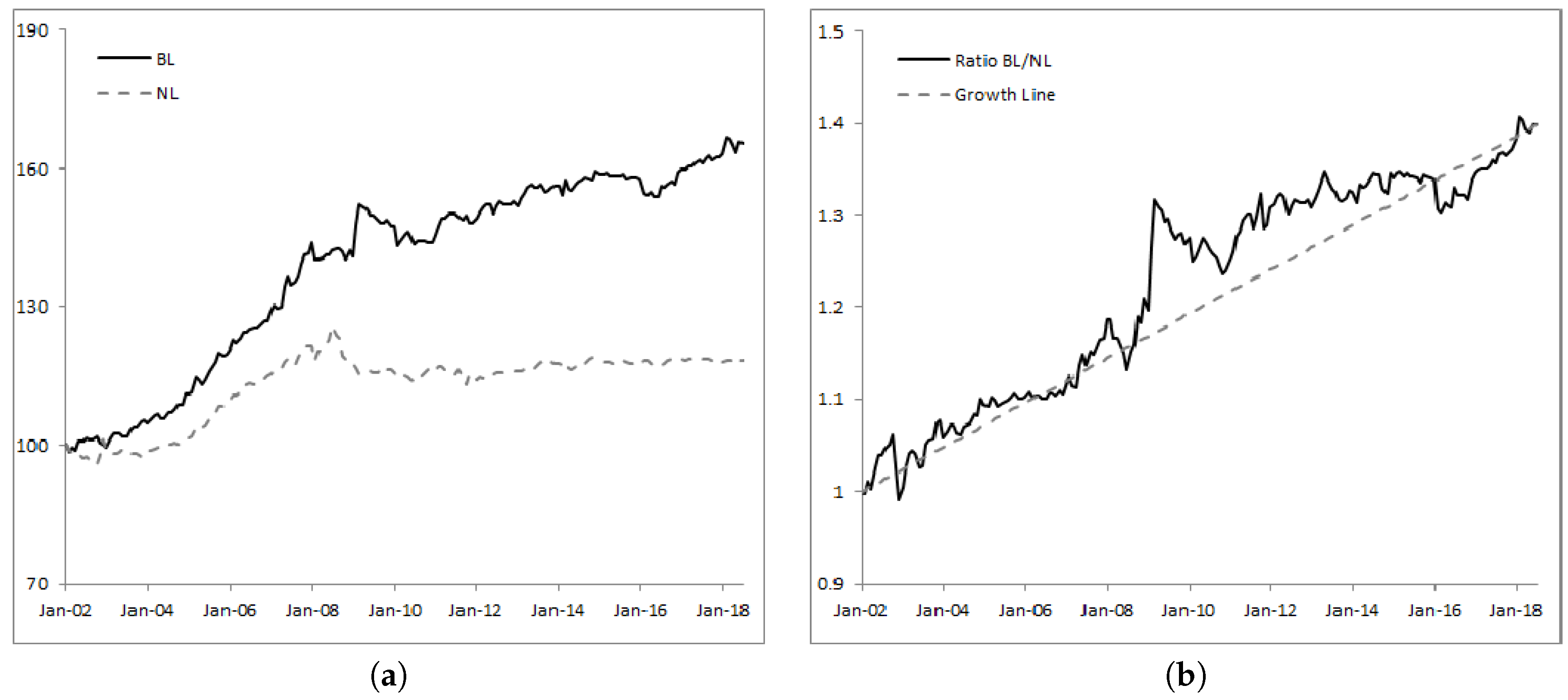
Figure 7 shows the historical performance (
Figure 7a) and the strength ratio (
Figure 7b) of the
BL strategy over
NL. Clearly, learning over time produces regular outperformance, as shown by the regular upwardly increasing ratio between
BL and
NL.


