1. Introduction
During the last decades, mortality has significantly declined in most developed countries around the world, mainly due to the continuous improvement of living conditions and the evolution of medical science and technology. This decline in mortality results in a steady increase of life expectancy, which creates higher financial responsibilities for governments and annuity providers. Consequently, finding ways to manage the mortality dynamics of a population is a very important step in building a sustainable health and pension system. In this spirit, actuaries and demographers have focused on the development of novel methods to model and forecast the mortality rates of a population.
Lee and Carter (
1992) proposed a pioneer modelling method to forecast the mortality of the total population of the United States, by decomposing the mortality rates into two age and one period parameters. A remarkable variant of the Lee–Carter method, particularly designed for higher ages, was proposed by
Cairns et al. (
2006), who incorporated two period parameters. In the literature, we can find many extensions to these methods.
Renshaw and Haberman (
2006) extended the Lee–Carter model by including a cohort effect, while
Cairns et al. (
2009) added a cohort parameter to the
Cairns et al. (
2006) model. In addition,
Plat (
2009) proposed a model which combines preferable characteristics of the
Lee and Carter (
1992) and
Cairns et al. (
2006) models.
An issue that sometimes appears in mortality modelling is that, for some countries, there are too few data to fit. This issue affects the existing modelling methods, which inevitably base their forecasts on population datasets of a limited historical period of observations. In the literature, there are extensions of the Lee–Carter method that can be utilized when dealing with limited datasets. For instance,
Li et al. (
2004) extended the Lee–Carter model to be applied for Chinese and South Korean mortality data, which are available at only a few points in time and at unevenly spaced intervals.
Zhao (
2012) modified the Lee–Carter model by incorporating linearized cubic splines and other additive functions to approximate the model parameters and forecast mortality for short-base-period Chinese data and
Huang and Browne (
2017) presented a stochastic modification of the CMI (Continuous Mortality Investigation) model to project mortality improvement rates for limited Chinese data using clustering analysis techniques.
Recently, some alternative modelling approaches have also been proposed as a tool in mortality forecasting. Differently from the above Lee–Carter variants and extensions, these approaches are based on credibility theory, aiming to model the period patterns of limited mortality data for a specific age, using useful information from a wider age span.
Bühlmann (
1967) established the theoretical foundation of modern credibility theory (also known as greatest accuracy credibility theory), which is widely used in non-life insurance and
Hachemeister (
1975) introduced a credibility regression model to estimate auto-mobile bodily injury claims for various states in the USA.
Credibility regression has a long history in credibility literature, with applications mainly in non-life insurance:
De Vylder (
1978) proposed estimators for the structural parameters in a more general regression model;
Norberg (
1980) proposed empirical credibility estimators under various model assumptions and established asymptotic optimality;
Ledolter et al. (
1991) derived a credibility method that allows for time-varying parameters in the process; and
Pitselis (
2004) presented the relationship between claim amounts and a set of explanatory variables into a credibility regression model with cross-section and time effects, with applications for general insurance data. For an extensive review on credibility theory for non-life insurance, we also refer to the works of
Goovaerts et al. (
1990);
Bühlmann and Gisler (
2005) and
Klugman et al. (
2012).
Regarding some life insurance applications of credibility theory,
Hardy and Panjer (
1998) used empirical Bayes credibility theory to provide a theoretical basis for the calculation of risk measures associated with mortality risk for insurance companies.
Salhi et al. (
2016) proposed a credibility approach, which consists on reviewing the fitting parameters of a Makeham mortality curve, as new observations arrive.
Schinzinger et al. (
2016) presented a multivariate evolutionary credibility model for mortality improvement rates to describe the joint dynamics of mortality through time in several populations. Moreover,
Li and Lu (
2018) proposed a Bayesian non-parametric model for the mortality of a small population, when a benchmark mortality table of a larger population is also available and serves as part of the prior information. By using an adaptive smoothing procedure based on the local likelihood,
Salhi and Thérond (
2018) proposed a methodology to adjust the graduated mortality table based on credibility techniques. In addition,
Gong et al. (
2018) highlighted the importance of using credibility procedures in individual life and annuity business.
Two recent contributions to modelling mortality under a credibility framework were also made by
Tsai and Lin (
2017a,
2017b). In the first paper, they applied Bühlmann credibility to mortality data of Japan, the United Kingdom and the United States, while, in the second one, they incorporated Bühlmann credibility into the
Lee and Carter (
1992) model, the Cairns–Blake–Dowd model (
Cairns et al. 2006) and the linear relational model of
Tsai and Yang (
2015) to improve forecasting performance for the United Kingdom dataset. However, it has been observed that the age-specific mortality rates show a clear downward trend over time. Moreover, when we have limited mortality data experience for a specific age, but extensive data experience for the entire age range, the use of credibility regression techniques should be preferred to capture mortality trends. Our work aims to exploit the advantages of credibility regression compared with the most widely used mortality models, as an alternative to Bühlmann credibility, to forecast the mortality rates, especially for populations with limited data.
The rest of this paper is organized as follows.
Section 2 briefly reviews the Lee–Carter, the Cairns–Blake–Dowd and the random coefficients regression models.
Section 3 proposes a credibility regression approach with randomly varying coefficients and a special case with fixed coefficients to model mortality rates.
Section 4 presents the extrapolation methods used to estimate future mortality rates under the credibility regression approaches. An empirical illustration using Greek male and female data is presented in
Section 5.1, in which forecasting performances of credibility regression, and the Lee–Carter and Cairns–Blake–Dowd methods are evaluated with the
MAFE and
RMSFE measures. A comparison between Bühlmann credibility and credibility regression forecasting methods is also presented in
Section 5.2 and an application on pricing insurance-related products follows in
Section 5.3. Finally, concluding remarks are discussed in
Section 6.
2. Mortality Modelling: A Review of Methods
In this section, we briefly review the Lee–Carter model, the Cairns–Blake–Dowd model and the random coefficients regression models that will be utilized in next sections.
2.1. The Lee–Carter Model
In its original form, the Lee–Carter (LC) model links the natural logarithm of the observed mortality rates
with the following model predictor:
where
is an age parameter that reflects the average mortality at age
,
is a period parameter which indicates the general level of mortality in year
and
is an age parameter that indicates the deviation from the average mortality at age
, as the general level of mortality changes. The errors
are expected to be normally distributed, with zero mean and constant variance, reflecting specific period and age effects not captured by the model. Thus, after assuming that errors are independent and homoscedastic with zero mean,
Lee and Carter (
1992) suggested a close approximation to the SVD (Singular Value Decomposition) method, under the constraints
and
, to obtain the following parameter estimates:
Later on, to allow for heteroscedasticity in error variance,
Brouhns et al. (
2002) assumed that
follows a Poisson distribution with mean
. Under this approach, age and period parameters are estimated by maximising the log-likelihood function of (
1).
After choosing one of the above estimation approaches, period estimates are extrapolated using time series methods.
Lee and Carter (
1992) suggested a random walk with a drift parameter
to project period parameter for
years ahead, according to
. Then, projected
s are utilized along with the estimates of age parameters
and
to obtain the following mortality forecasts:
2.2. The Cairns–Blake–Dowd Model
The Cairns–Blake–Dowd (CBD) model links the logit transformation of one-year probabilities of death
with the following model predictor:
where
is a period parameter which indicates the general level of mortality in year
and
is a period parameter that shows how mortality affects each age, while
is the mean age of the considered fitting age interval and
reflects specific effects not captured by the model and is expected to be normally distributed, with zero mean and constant variance. Again, we briefly present the estimates of the model parameters, which can be obtained by regressing
on
for each
:
Alternatively,
Cairns et al. (
2009) assumed that deaths follow a Poisson distribution with mean
, where
. Then, the CBD model parameters are obtained by maximizing the log-likelihood function of (
3). Assuming that period estimates are independent, each one of them is extrapolated using a random walk with a drift parameter (
) and then mortality forecasts for
are obtained by
Remark 1. We can easily observe that expressions in Equations (2) and (4) are both linear functions of the forecasting horizon , where their intercepts are equal to the fitted rates of the last observed year and their slopes are the products of the estimated age parameters with the drift terms. 2.3. The Random Coefficients Regression Model
Empirical data indicate that mortality in each age decreases linearly over time. Especially in higher ages, mortality rates have been significantly improving over the last few years. We are interested in a model structure able to capture the improvement trends and describe the mortality evolution through time. For this reason, we consider a regression structure with random coefficients, aiming to capture the underlying mortality effects that are not included in the explanatory variables.
For each age
, the regression model with random coefficients is defined by
, where
is the response variable,
are the randomly varying coefficients and
are the explanatory variables. Then, each coefficient element can be decomposed in
, for all
and
, with
and
being the fixed and random parts, respectively, assuming that
,
for all
and
for
and
. For more details on regression models with random coefficients, we refer to the works of
Hildreth and Houck (
1968);
Hsiao (
1986) and
Greene (
2012).
The above formulation means that the unknown regression coefficients can take different values over an observed period. Actually, mortality dynamics for a specific age can vary over time, due to unknown or exogenous
1 factors.
Nevertheless, the random coefficients regression model may be reduced to a fixed coefficients model with heteroscedastic variances, defined as
where
for all
and
, with
.
We have to point out that error variances and cannot be identified separately, while the sum () can. Therefore, without loss of generality, is dropped and the above variance is simplified to . Note that variance heteroscedasticity is still present even if for , due to the existence of squared explanatory variables .
3. Credible Regression Mortality Models
In this section, we propose a mortality modelling approach embedded, for the first time, in a credibility regression framework with varying coefficients. The parameter estimation procedure is described and a special case with fixed coefficients is also provided.
3.1. A Credibility Regression Approach with Randomly Varying Coefficients
Denote as the observed number of deaths at age in year and as the average population aged during year (also called as population exposure to risk). Then, age-specific mortality rates are obtained by the ratio and one-year probabilities of death can be derived from the identity , which is implied by the assumption of a constant force of mortality over each year of integer age and over each calendar year.
We assume that response variable refers to an appropriate transform ( or ) of a mortality measure [ or ] for age of year , where variable corresponds to consecutive integer ages ( in total) and corresponds to consecutive calendar years ( in total). We also consider as an age-related random risk parameter, as a mortality vector and as the design matrix of explanatory variables. We note that, in general, the design matrix could consist of various explanatory variables that reflect mortality characteristics. For instance, in a medical study, mortality may depend on various factors, such as the genetic background of an individual aged , the life style, the nutrition, the toxicity of the environment, a possible infectious cause (bacteria, parasites, or fungi) or other socio-demographic factors that should affect mortality dynamics. Therefore, the pair that describes mortality evolution in age is , under the following assumptions:
- (i)
The pairs , , , are independent and are independent and identically distributed.
- (ii)
, where is a fixed design matrix of full rank and is an unknown regression vector of length .
- (iii)
,
or in matrix formulation:
= .
The structural parameters are defined as follows:
In such a regression setting,
has to be estimated. Consequently, instead of the ordinary least squares method, regression coefficients are estimated with the generalised least squares method (
GLS). Then, an individual estimator of
can be obtained by
Proposition 1. Under the above assumptions, the credibility estimator of is given bywithwhere is given in (8), and are defined in (7), and is the identity matrix. Proof. The mean square error of (
9) can be defined in terms of the norm
as
where
and
Using the product rule and differentiating with respect to matrix
, we have
By substituting the values of
and
and setting (
12) equal to zero, we obtain
which yields (
10). □
Then, the credibility estimator of future mortality rates
may be compactly written as
where
denotes the design matrix of future periods.
3.2. Estimation of Structural Parameters
To estimate the structural parameters of the random coefficients credibility regression model, we can proceed similarly as in
Hildreth and Houck (
1968). Let
be the vector of the least squares residuals from the regression of
on
given
, which is obtained by
where
is the least squares estimator of coefficients in ordinary regression,
is a symmetric and idempotent matrix of order
and
is the error term. Then, given
, the variance matrix of
, via (
6), becomes
from which we can get
where
,
and
are the Hadamard products of matrices
,
and
, respectively, while
is as defined in (
7). In addition, (
16) implies that, for given
, least squares residuals
are regressed on
, which yields
where
and
is a
disturbance vector, such that
. Hence, its variance-covariance matrix is given by
where
represents the Hadamard product of matrix
by itself, with
Then, if
s are known, the
GLS estimator of
in (
17) is obtained by minimising the criterion function
, which gives
However, estimators of
in (
8) and
in (
19) are non-operational, because the variance-covariance matrices
and
are functions of unknown variances. Therefore, operational estimators of
and
can be obtained by replacing unknown matrices with estimators
and
, respectively. A least squares estimator of the unknown variances
is directly obtained from (
17) as follows:
where equality
holds true, since
for a symmetric matrix
.
Remark 2. In the actuarial literature, there are many other types of estimators for variance in (17). For instance, Hildreth and Houck (1968) suggested the unbiased estimator , while Rao (1973) proposed the so-called “Minimum Norm Quadratic Unbiased Estimator” (MINQUE), given by . The random coefficients (
RC) credibility estimator of
, denoted as
, is given by
where
and
with
obtained according to (
7), by using the mean of the estimated variances in (
20). Future mortality estimates follow from
where
is the corresponding credibility factor. We suggest the following estimators for parameters
,
and
to obtain
De Vylder’s (
1978) optimality (minimum variance within the class of unbiased estimators):
and
Note that the estimators of
and
are implicit functions of the parameter to be estimated and should be calculated iteratively, by imposing
to retain symmetry after each iteration.
3.3. Credibility Regression with Fixed Coefficients and Weights: A Special Case
In the case of fixed regression’s coefficients, the previous model reduces to a special case of
Hachemeister’s (
1975) model with no weighs, i.e.,
. In particular, some weights may appear in each regression line of
. For instance, population exposures
, for
can be used as weights. In this case, we have the standard regression case of Hachemeister’s model. To proceed, we follow the same Assumptions (i) and (ii) as in the random coefficients case, but covariance matrix in Assumption (iii) is simplified to
, where
is a fixed
positive definite diagonal matrix, with weights
. The structural parameters are now defined as
and the ordinary least squares estimator of the coefficients vector
is given by
and the variance-covariance matrix is obtained by
, while its expected value is given by
Based on the above assumptions, the credibility estimator
of
for the fixed coefficients (
FC) model is given by
where
is the estimated credibility factor. Similarly, for the derivation of (
28), we refer to
Bühlmann and Gisler (
2005). To recapture
De Vylder’s (
1978) optimality, we use the following estimators:
Again, the estimators of
and
should be calculated iteratively, imposing
after each iteration.
4. Extrapolation Methods for Estimating Future Mortality Rates
In this section, we fit the random coefficients (RC) and the fixed coefficients (FC) credibility regression models to mortality rates for age of year . For both models, the fitted rates up to year can be compactly written as . As we noted before, design matrix could consist of various independent variables that reflect risk factors for any given age , but due to lack of specific data, we assume that s for each given age , depend only on the period effects of each calendar year, i.e., . However, if specific data are available, for instance in case of life insurance datasets, then more explanatory variables can be incorporated in the regression model. Henceforth, we consider the same design matrix for all s.
4.1. Standard Extrapolation Method (SEM)
Based on current fitting data of the response variable
, mortality rates for one-year ahead are estimated by
Similarly, estimates of future mortality rates for age
are given by extrapolating one-year ahead estimates in (
32) to
, for
, where the credibility estimators
are obtained by (
21) for the RC or (
28) for the FC model. Hence, under this method, future estimates are based on the mortality data of the initial fitting span
.
4.2. Other Extrapolation Methods
In practice, two additional methods can also be used to extrapolate mortality rates over a given forecasting horizon . Thus, for each one of the RC and FC models, one-year ahead estimates can be embedded to the existing fitting span, with simultaneously excluded from it, so that the fitting year span is moved forward by one year each time to , , , . Then, after repeating the estimation procedure, we can consecutively obtain , . Under this “moving extrapolation method (MEM)”, future estimates are based on more recent mortality trends.
Alternatively, one-year ahead estimates
can be embedded to the existing fitting span, without removing
, so that the fitting year span is extended by one year each time to
,
,
,
. Hence, in each estimation step, credibility regression models are fitted on a continuously extended response variable, to obtain
,
,
. Under this “extended extrapolation method (EEM)”, future mortality trends are based on both the initial mortality rates and the recent ones that have been obtained after each estimation step. Similar practical approaches have also been adopted by
Luan (
2015). The numerical results in the following section justify that all methods can be efficiently applied in actuarial practice.
Remark 3. Similar extrapolation methods may be used in other regression or time series contexts, but here are customized to be used with the credibility regression models presented in Section 3. 5. Empirical Illustration
In this section, the Lee–Carter (LC), the Cairns–Blake–Dowd (CBD) and the credibility regression models are fitted on Greek mortality data. Then, forecasting results are evaluated using the mean absolute forecast error (
MAFE) and the root mean of squared forecast error (
RMSFE) measures. Greek data have a limited number of historical mortality observations (1981–2013), which are available on the
Human Mortality Database (
2017), structured by year, age and gender. Furthermore, in life insurance datasets similar limitations frequently exist. Credibility regression can efficiently capture the underlying data trends, especially in cases where there is limited mortality experience for a specific age, but extensive experience for the entire age range (the case of Greek data). Of course, credibility regression methods can also be used for larger datasets.
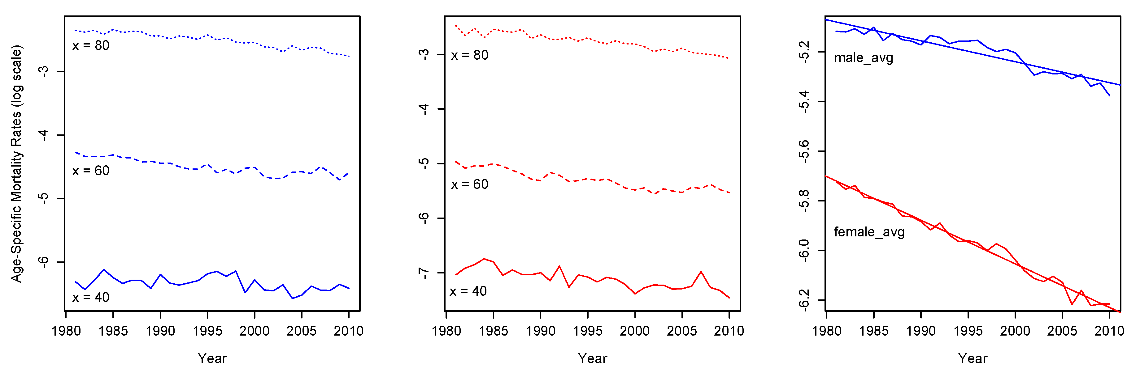
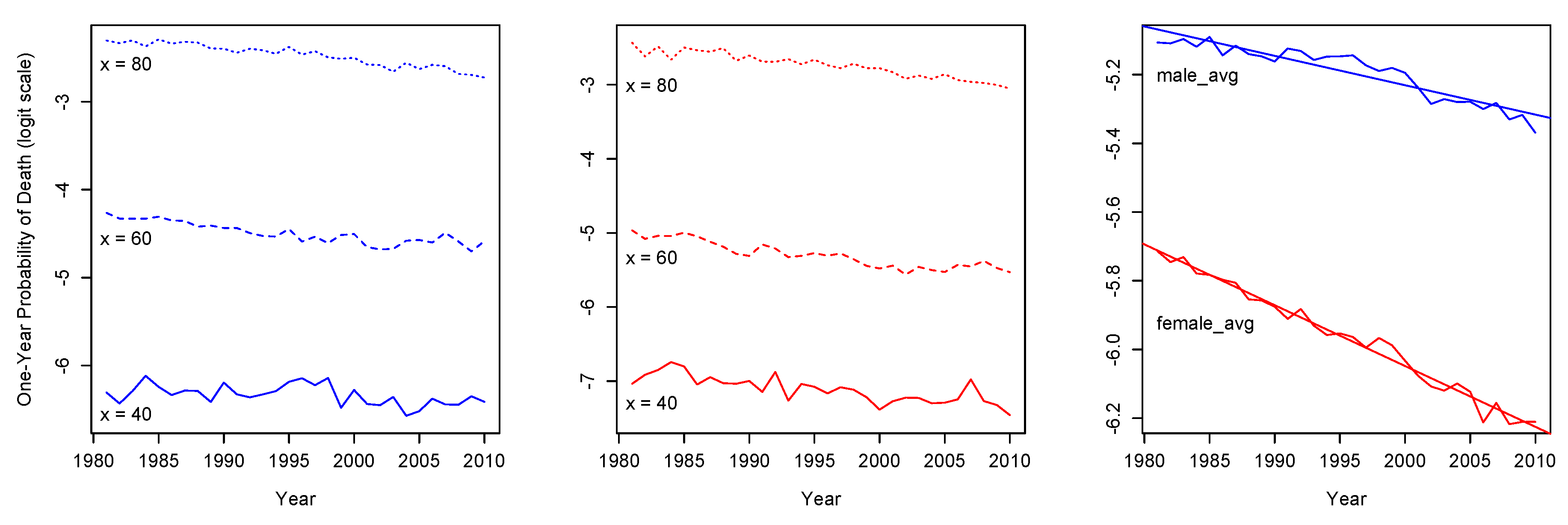
Mortality evolution for the period 1981–2010 in Greece is illustrated in
Figure 1 and
Figure 2 for
and
, respectively. Both mortality measures show a linearity for discrete ages
of males (left panels of
Figure 1 and
Figure 2) and females (middle panels of
Figure 1 and
Figure 2). In addition, for both genders, average mortality decline shows a clear downward trend over time (right panels of
Figure 1 and
Figure 2).
5.1. Forecasting Results
For the numerical illustration that follows, we used the empirical age-specific mortality rates
from 1981 to 2010, for males and females at the ages of 15 to 84. This age span choice is in accordance with similar studies (
Tsai and Lin 2017a,
2017b) as it corresponds to the age of a young adult up to the overall level of life expectancy in developed countries. To ensure robustness, relative to changes in the fitting range of data, we used two age and three period spans to extract forecasts for a 10-year
forecasting horizon, presented in
Table 1. In particular, for the FC model, we used
as weights. The credibility regression methods, as well as the LC and the CBD mortality models, were implemented in R (
R Core Team 2017). In particular, for the Poisson LC and CBD fitting methods, we used the “LifeMetrics” R package
2.
To retain linearity over each corresponding fitting period, the logarithmic transform
was used for the age-specific mortality rates and the logit transform
for the one-year probabilities of death. Forecast errors were then evaluated over the 10-year forecasting horizon using
MAFE and
RMSFE measures
3, where smaller values indicate a better forecasting performance. Averaged (avg)
MAFE and
RMSFE values are obtained by using
and
Similarly, in the case of using
as response variable,
should be replaced by
in above formulas. Forecast accuracy results at percentage (%) scales are evaluated over the period
.
MAFE and
RMSFE values for fitting ages
, using
are illustrated in
Table 2 (a) and (b), respectively, while the corresponding values for ages
with
are presented in
Table 3 (a) and (b), respectively. Note that CBD model is included only for comparisons in fitting ages
, as it has been particularly designed for higher ages.
For both genders, accuracy results in
Table 2 (a), (b) for fitting ages
and
Table 3 (a), (b) for ages
indicate that, for each fitting period, credibility regression models outperform LC and CBD models for both error measures. Average values over the whole period are given in the last rows of each measure’s subtable. More precisely, for ages
, the FC-MEM and FC-SEM produce the smallest average
MAFE and
RMSFE, while for ages
, RC-MEM performs better in average under both measures, which indicates that forecasts for higher ages are based on more recent mortality trends. Moreover, we observe that errors are getting evidently larger, when shortening the age fitting span to
. This is due to the fact that both
in (
33) and
in (
34) are generally increasing with age
. Therefore,
and
for ages
are larger than those for
.
We note that, for our comparison, we used the Lee–Carter (
1992) and Cairns–Blake–Dowd (
2006) models, which incorporate only age and period effects. Models with cohort parameters were intentionally excluded from our analysis to be consistent with the age-period structure of the proposed credibility regression methods that model the period dynamics of mortality across the ages. For a modelling comparison study on Greek data that allows for models with cohort effects, we refer to the work of
Bozikas and Pitselis (
2018).
Credibility Effects on Mortality Modelling
In the preceding section, we used the proposed credibility regression methods to estimate the actual mortality trend for a specific age, by weighting the mortality trend for this age and the mean trend over a wider group of ages that encompasses much more information.
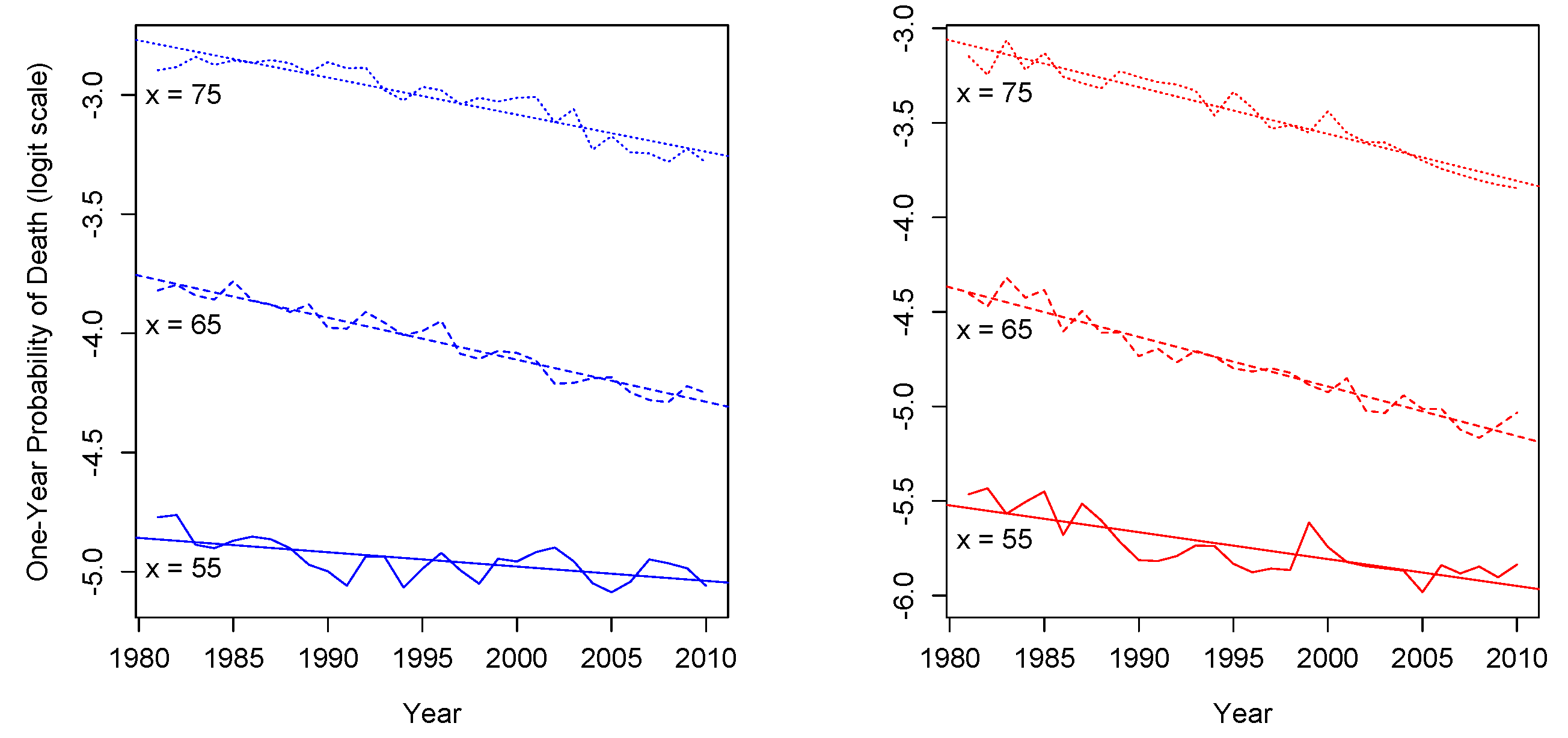
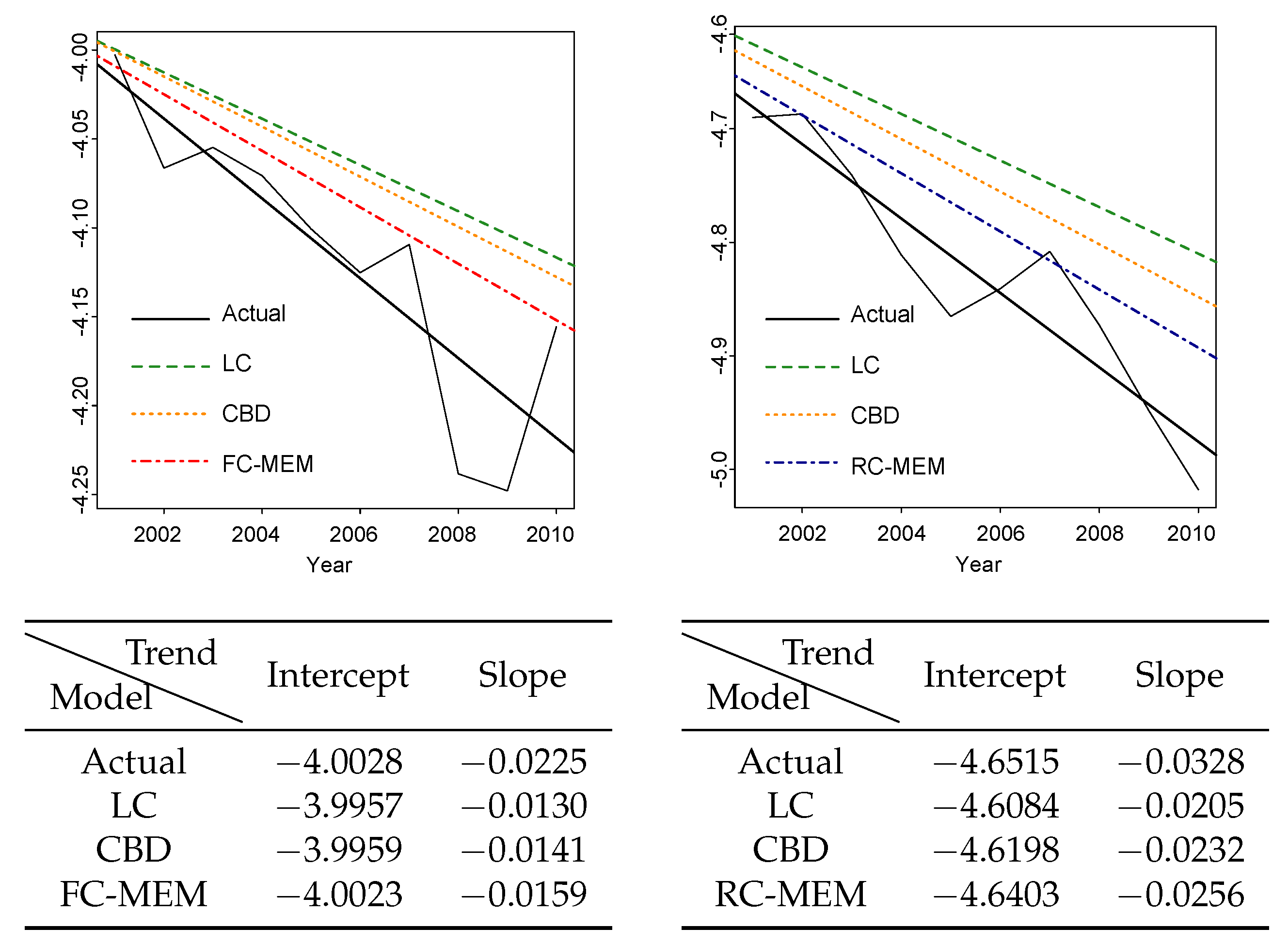
Figure 3 illustrates the linear trend of the actual (observed)
for Greek males (left panel) and females (right panel), aged 55, 65 and 75 over the period 1981–2010. The intuition behind using credibility regression is that the proposed methods could potentially lead us to more accurate estimates for the intercept and the slope of the mortality curve for a given age
. To assure this, we used the absolute forecast errors by age (
) to compare the linear trend (intercept and the slope) of the
,
between the actual rates and the rates produced from the best performing models for both genders over years
, with and without credibility, for pension ages
, fitted for
. For each model,
can be obtained by
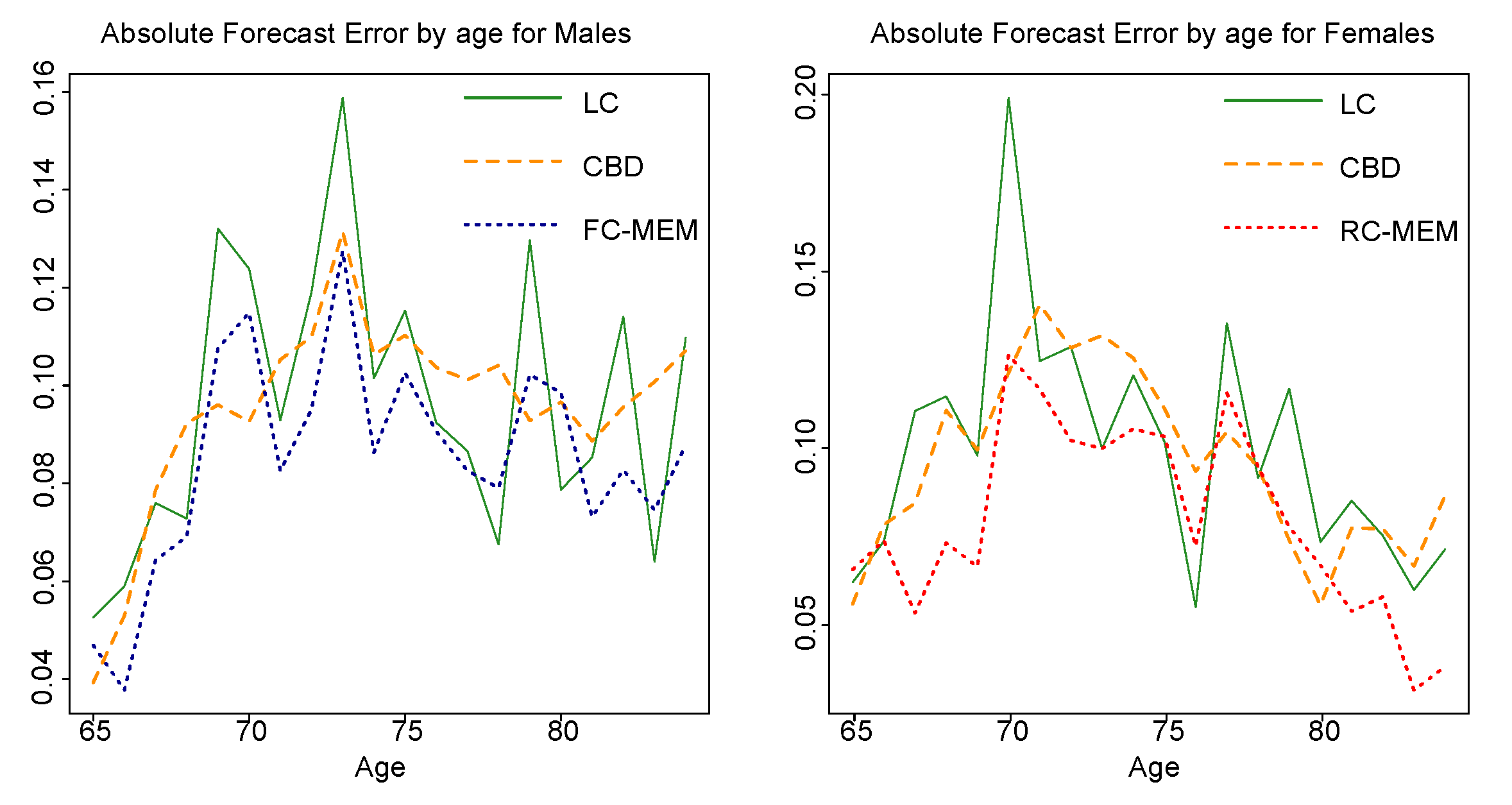
Figure 4 displays the
comparison results, which indicate that, almost for all ages, credibility regression methods (dot lines) perform better than the LC (solid lines) and CBD (dashed lines) models. An alternative way to see how close the credibility forecasts are to the the actual mortality trend,
Figure 5 illustrates the intercept and the slope of the actual rates and the forecasted ones for some ages, under the best performing methods (based on
) with credibility (FC-MEM for males and RC-MEM for females) and without credibility (LC, CBD).
The trend lines for the RC-MEM and FC-MEM forecasts can be easily extracted using the ordinary least squares method. Recall that, the intercept and the slope for the LC and CBD models is given by Equations (
2) and (
4), respectively (Remark 1), while for the credibility method RC by (
21) and for FC by (
28). The illustrated results in
Figure 5 indicate that intercepts and slopes of the FC-MEM (for males) and RC-MEM (for females) lines are closer to the actual ones, which set the best starting point for the forecasts.
5.2. Applying the Bühlmann Credibility Approach
Tsai and Lin (
2017a) proposed a Bühlmann credibility approach to forecast mortality rates for both genders in Japan, the United Kingdom and the United States. This model can be directly obtained from the more general regression model, presented in
Section 3.3, if we set
and
for
. Then, from (
27),
is equal to
and the model parameters, which are scalars now, can be estimated by
The Bühlmann credibility estimates for one year ahead can be obtained by
In contrast to the credibility regression approaches, which aim to capture the downward trend of
s over
, for the Bühlmann credibility approach to be applied, this downward trend must be eliminated. For this reason,
Tsai and Lin (
2017a) applied the Bühlmann credibility model on the time series of mortality rate changes rather than the mortality rate levels, i.e.,
, for
. Then, they proposed two strategies for estimating
,
. The first strategy expands fitting window (EW) by one year, similarly with the EEM regression method, described in
Section 4 and the second one moves fitting window (MW) by one year, similarly with the MEM regression method. In what follows, we compare the forecasting performance between the Bühlmann and the credibility regression methods on Greek data. To be consistent with the Bühlmann modelling framework of
Tsai and Lin (
2017a), age fitting spans [21, 85] and [56, 85] were selected and forecast errors were also evaluated under the averaged
MAPFE values, which is defined by
Error values for each gender were evaluated by fitting
s on [1982, 2000], [1986, 2000], and [1990, 2000] period spans. Comparison of averaged
MAFE,
RMSFE and
MAPFE4 results between Bühlmann and credibility regression methods is given for both genders in
Table 4 (a)–(c) for ages [21, 85] and
Table 5 (a)–(c) for ages [56, 85].
The results indicate that credibility regression methods produce the smallest
MAFE,
RMSFE and
MAPFE values for the majority of the selected fitting periods for both age spans. More precisely, the FC-MEM method has the best average performance according to
MAFE and
MAPFE values for ages [21, 85], while the RC-MEM method seems to be more appropriate to capture future mortality trends for older ages [56, 85]. We note that the smallest values in average are produced by different regression methods, depending on which measure is used. Such inconsistencies are expected due to the nature of
MAFE,
RMSFE and
MAPFE formulas. That was also pointed out by (
Tsai and Yang 2015, p. 9).
5.3. Application in Insurance-Related Products
In this section, we apply the mortality forecasts obtained from the Lee–Carter, the Cairns–Blake–Dowd and the credibility regression models to calculate life premiums, reflecting the appropriateness of each model in pricing applications. Denote
as the fully discrete life insurance premium, payable at the end of the year of death, if it occurs within a term of
years and
as the pure endowment, payable at the end of
years in case of being alive. Both products are issued to an insured aged
in year
. Net premiums (NP) are obtained (see
Bozikas and Pitselis 2018) by
where
denotes the
k-year survival probability for age
in year
, while its estimate is given by
,
and similarly for
, where
is the interest rate and
. In addition, to see the performance on a life annuity product, typically used for pension applications, denote
as the discrete life annuity-due at age
in year
, payable annually for up to
years. Its actuarial present value (APV) can be obtained by
Then, we apply the estimated mortality rates obtained from the LC, CBD and credibility methods, fitted to 1981–2000 rates, to calculate the NPs and APVs for ages 55–74 with
, assuming
. The errors between forecasted values and those produced from the observed mortality rates for the years 2001–2010 are evaluated using
MAFE and
RMSFE, which are defined by
Similarly,
MAFE and
RMSFE formulas are adjusted for pure endowment or annuity products by replacing
with
or
in Equations (
44) and (
45).
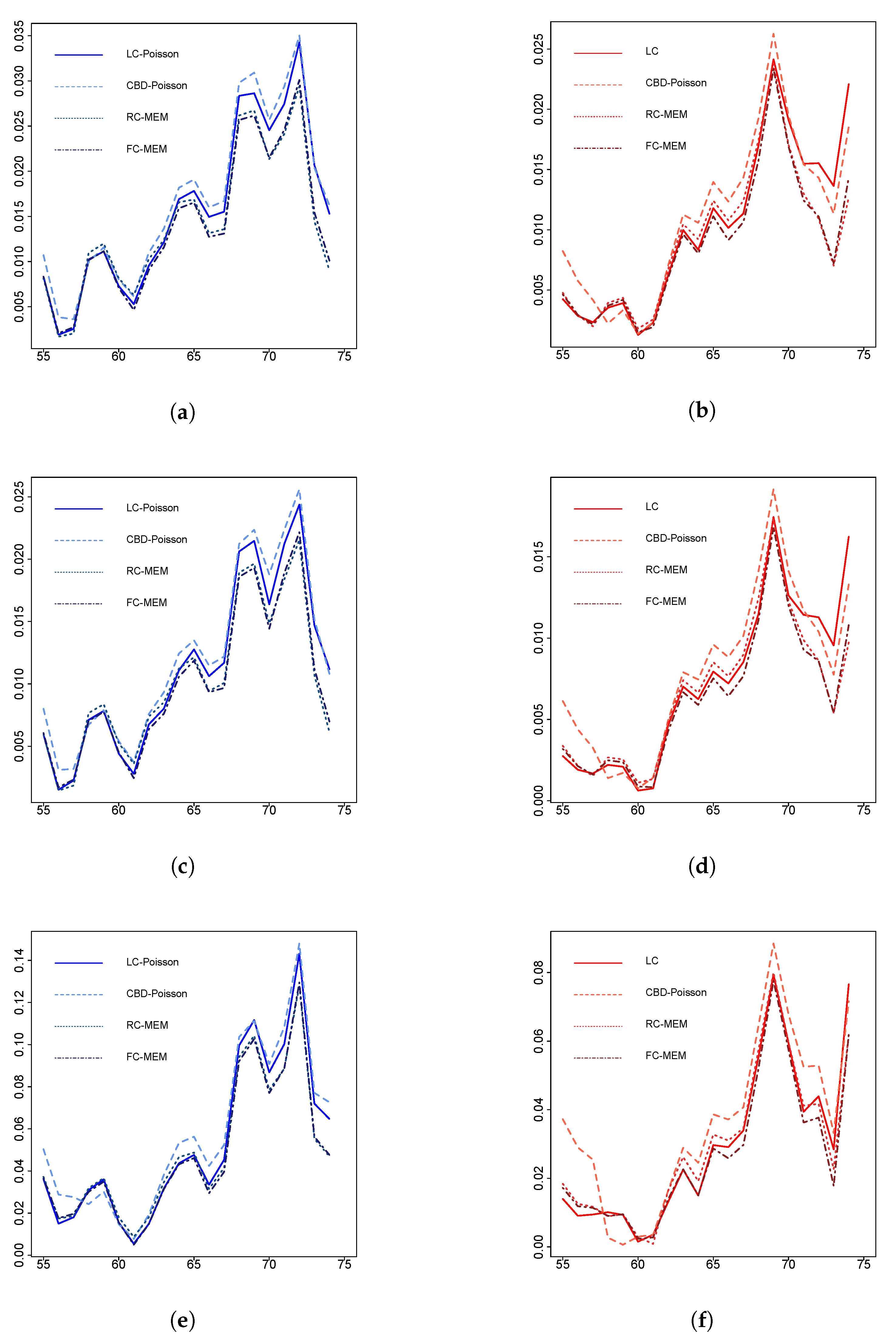
Table 6 presents the averaged error values in ranking order for a 10 year forecasted life insurance, pure endowment and life annuity for both genders, aged 55–74 in 2001–2010. In addition,
Figure 6 illustrates the absolute forecast error values against each corresponding age (
) for the top LC, CBD, RC and FC credibility regression methods for males and females, according to
Table 6 values. For each model,
is obtained from
.
According to
MAFE and
RMSFE values for both genders and insurance products in
Table 6, credibility regression models produce better insurance-related forecasts in comparison with the LC and CBD modelling methods. We can easily observe that for each gender, error measures coincide in the same ranking order for all insurance products. In particular, measures show that credibility regression methods under a moving fitting span outperform LC and CBD methods in aggregate, with FC-MEM being dominant and RC-MEM following. This fact is also evident in
Figure 6, where absolute error values against age for the MEM regression models lie on the lower levels for all the insurance products. Nevertheless, the FC-SEM should also be a good modelling choice for pricing insurance-related products.
6. Concluding Remarks
Credibility regression techniques seem to be of special interest and particularly useful for mortality datasets of a relatively short historical period of observations (limited data), as they can efficiently capture the underlying mortality trend for a given age, using all the information gained from populations of other ages. This paper proposes mortality modelling approaches embedded, for the first time, in a credibility regression framework. In our illustration on Greek data, credibility regression approaches resulted in better forecasts for both genders (in terms of
MAFE and
RMSFE measures), compared to the Lee–Carter and Cairns–Blake–Dowd models, as well as the Bühlmann credibility approach (
Tsai and Lin 2017a). Finally, their performance was also evaluated on insurance-related applications.
Specifically, in
Section 3, we proposed a credibility regression mortality framework with randomly varying coefficients and a special case with fixed coefficients. To estimate future mortality rates, we presented extrapolation methods for each credibility approach in
Section 4. The applicability of our modelling approaches was comparatively illustrated on Greek male and female data in
Section 5, accompanied with an explanation of the credibility effects in mortality modelling and a pricing application on insurance-related products. From our analysis, we concluded that, in aggregate, credibility modelling methods performed better than the LC and CBD methods. Forecasting accuracy results indicate that, for the whole age fitting span, fixed coefficients credibility methods performed better on average, while, for higher ages, the RC-MEM should also be a good choice. In addition, the FC-MEM performed a bit better in aggregate on pricing insurance-related products.
Furthermore, we noted that FC-SEM credibility forecasts were closer to observed rates for the same periods, when we used population exposure to risk as weights, i.e.,
, but weighted regression is restricted for use only under the SEM, as
s are practically unknown for the upcoming years. Additionally, during the estimation procedure for the random regression models, we observed that, if we use the MINQUE estimator (Remark 2) instead of (
20), error values for all the credibility modelling methods become even smaller for both genders.
For the sake of comparability, the Bühlmann credibility approach (
Tsai and Lin 2017a) was applied on our dataset in
Section 5, where the credibility regression methods resulted to better forecasts based on
MAFE,
RMSFE and
MAPFE measures. In addition, credibility regression methods had a very good forecasting performance, when we applied them to the datasets of other countries (with a relatively small population
5) for a limited selected fitting period (1980–2000), such as Belgium, Finland, Norway, Ireland, Slovakia and New Zealand. A further forecasting comparison between datasets of other countries has been left for future work.
Finally, we have to mention that our numerical illustration yielded results that are fully applicable and provide encouragement that credibility modelling approaches, including those of
Tsai (
2017a,
2017b), could contribute to future mortality projection studies.
