An Indexation Mechanism for Retirement Age: Analysis of the Gender Gap

Abstract

The management of National Social Security Systems is being challenged more and more by the rapid ageing of the population, especially in the industrialized countries. In order to chase the Pension System sustainability, several countries in Europe are setting up pension reforms linking the retirement age and/or benefits to life expectancy. In this context, the accurate modelling and projection of mortality rates and life expectancy play a central role and represent issues of great interest in recent literature. Our study refers to the Italian mortality experience and considers an indexing mechanism based on the expected residual life to adjust the retirement age and keep costs at an expected budgeted level, in the spirit of sharing the longevity risk between Social Security Systems and retirees. In order to combine fitting and projections performances of selected stochastic mortality models, a model assembling technique is applied to face uncertainty in model selection, while accounting for uncertainty of estimation as well. The resulting proposal is an averaged model that is suitable to discuss about the gender gap in longevity risk and its alleged narrowing over time.

1. Motivation

In this paper, we wish to contribute to the existing literature by adopting an indexation mechanism for retirement age: The proposal consists in the computation of lags to be applied to a benchmark retirement age in order to keep a constant expected pension period duration (EPPD). Given this flexible pension system, we face the problem of dealing with the risk deriving from model selection by applying an assembling technique. Our study was carried out with reference to the Italian Mortality experience since Italy is characterized by a “Generous Pension System” (Sartor et al. 1999) and by life expectancy and pension spending among the highest in OECD (Organisation for Economic Co-operation and Development) countries. These features led to a hard sustainability of the Italian Social Security System given the projected demographic trends. The reason behind that, besides mortality trends, is also the design of the system. As Chlon-Dominczak et al. (2012) mention, the design (indexation and notional rate) is a cause of unsustainability in all Nonfinancial Defined Contribution (NDC) countries. They indicate, for instance, that “Italy would suffer deficit over long periods of time after just two or three negative shocks mainly due to the choice of the notional rate equal to the three-year GDP growth average.” Also, Alonso-García et al. (2018) indicate that the front-loading design in Italy and Sweden and the usage of a current life table (instead of a projected one) would lead to liquidity problems very soon. Given these motivations, the proposal can be adapted and applied to similar scenarios. The approach here pursued stems from the preliminary investigations addressed in Coppola et al. (2018a, 2018b) and it is invoked here to discuss the evolving issue of gender gap in life expectancy and its implications.

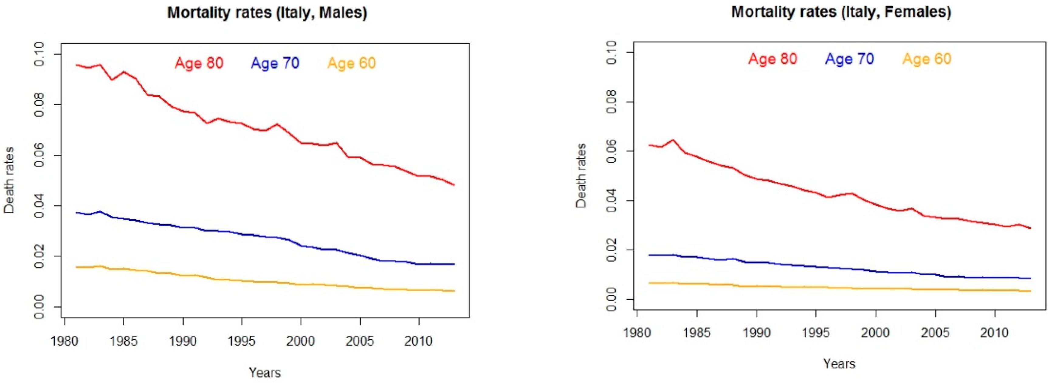
Indeed, when focusing on longevity risk, a popular and fundamental discussion concerns the understanding of why women live longer than men. Evidence from Italy is shown in Figure 1, where observed death rates for people aged 60, 70, 80 are displayed for males and females.

Then, in particular at older ages and thus when designing pension plans, the gender gap in longevity needs to be approached suitably. Most importantly, the decreasing decay of mortality for women and the resulting narrowing of the gender gap provide further support to the need of a flexible retirement scheme that could accommodate over time the different patterns of the mortality experience over time and gender.

The paper is organized as follows: after a concise overview of pension system sustainability, in Section 2 we illustrate a proposal of an indexed retirement age mechanism. In Section 3, we briefly describe the stochastic mortality models chosen to forecast mortality rates, in the framework of the generalised age-period-cohort (GAPC) family. Then, we consider the risk arising in the model selection phase. To this end, we implement a model assembling methodology which is particularly advisable since its application trades off fitting and prediction capabilities. Most importantly, given the narrowing of the gender gap in longevity and its evolution over time, the combination of an indexation mechanism and a model assembling technique could account for the longevity risk.

Conclusions and further developments complete the presentation. The implementation of the proposal is carried out in the R environment: The code is available upon request from the Authors. For the analysis, the R packages StMoMo (Villegas et al. 2018), Lifecontingency (Spedicato 2013), Demography and Forecast (Hyndman and Khandakar 2008) have been exploited.

Increasing Retirement Age and Pension Systems Sustainability

Nowadays the progressive improvement in life expectancy at advanced ages affects the developed countries so profoundly that it represents a central issue for governments in many different fields such as the National Social Security Systems. In particular, the trend of mortality is uncertain and this uncertainty causes the so-called Longevity Risk, which has become one of the key risks that Governments encounter in the context of social security welfare policies. As a matter of fact, people tend to survive beyond the retirement age for an average number of years exceeding the expectations and this leads to a crucial question for public finances. To deal with this problem, several countries in Europe have set up pension reforms linking the retirement age and/or pension benefits to life expectancy to foster the Pension System sustainability (to quote a few, Finland, Cyprus, Denmark, The Netherlands, Great Britain, according to: Finnish Centre for Pensions (2018).

Even if the forthcoming discussion will concern public pension schemes mainly, it is worth to recall that such debate is topical also for the actuarial private setting. For instance, Richter and Weber (2011) consider life annuities where benefits are linked to the actual mortality experience of a reference group: then, this indexing proposal is compared to a benchmark product in terms of longevity risk reduction. For mortality rates projections, they refer to the extensions of the Lee Carter model presented by Brouhns et al. in 2002 (Brouhns et al. 2002). Denuit et al. (2015) propose deferred annuity contracts, where the length of the deferment period is subject to re-evaluation for mitigating the systematic longevity risk.

Public pension systems, instead, are usually funded on a pay-as-you-go (PAYGO) basis, where pensions for retirees are paid by the contributions of the working-age population (Godínez-Olivares et al. 2016b). Bisetti and Favero (2014) study the impact of longevity risk on the Italian pension system by projecting future mortality rates with the Lee Carter model in its baseline version and considering the different regimes that have followed in Italy over time until the recent “Fornero Reform.” This Reform has two directives: the rise of the pensionable age, linked now to the life expectancy and the calculation of the requirements for retirement on the basis of the number of years of social security contributions paid and no longer on the average salary earned in the last years before retirement. In particular, the reform has changed the benefit formula, going from defined benefit (DB) to defined contribution (DC). However, the financing mechanism remains identical to the previous system (i.e., PAYGO). Contrary to a fully funded DC, redistribution is still based on the “rule” that current contributors finance current pensioners’ benefits.

It is clear that PAYGO pension systems need an “intergenerational solidarity,” that is, an equilibrium between the benefits paid to the pensioners and the contributions made by the active workers. At the same time it has to ensure a long-term sustainability, undermined by the decline in fertility rates and the increase in longevity, that contribute to a substantial growth in the old-age dependency ratio. Due to the enhancements in life expectancy, pensions have to be paid over a longer time horizon, causing great difficulties especially when the system does not expect such improvements (Godínez-Olivares et al. 2016a). A possible approach to react to changes in fertility and ageing is to introduce a contingency fund in order to absorb unexpected events that might affect the liquidity and the sustainability of PAYGO pension systems (Alonso-García et al. 2018). Godínez-Olivares et al. (2016a), define this fund as the intertemporal budget balance that equates expected future expenditures to expected future income from contributions. They discuss optimal strategies to ensure liquidity by changing contribution rate, retirement age and/or indexation of pensions and propose an Automatic Balance Mechanism to restore the liquidity of the system at the end of a 20-year horizon. In Godínez-Olivares et al. (2016b), instead, the Authors discuss optimal strategies to ensure sustainability by changing contribution rate, retirement age and/or indexation of pensions. In particular, the Authors propose two different automatic balancing mechanisms using nonlinear optimization techniques to restore the sustainability over a 75-year time horizon into a DB-PAYGO pension system while keeping the system liquid at all times.

In order to guarantee the sustainability of the PAYGO pension system, some countries have proposed risk-sharing mechanisms (RSM). In this perspective, Alonso-García et al. (2018) assess how contribution rates and indexation rates should change to ensure liquidity. They design flexible and tractable RSMs that involve changes in the contribution rate and/or indexation of pensions, to restore the sustainability of the different pension schemes. The Authors contribute to the debate on pension finance in the sense that, for the very first time, sustainability and its effect on adequacy and fairness are studied under a dynamic set-up.

2. The Indexation Mechanism for Retirement Age

In this section, we consider an indexation mechanism for retirement age in the context of the Italian National Social Security System. As explained in Section 1, the Fornero Reform changed the benefit formula from DB to DC but it did not change the financing mechanism where current contributors finance current pensioners’ benefits (PAYGO system).

Life expectancy represents a demographic indicator that is accessible and transparent to all, as discussed in Denuit et al. (2015). Based on current life tables, it is regularly released by the National Institute of Statistics or other public bodies. In this section, we propose an indexing mechanism for retirement age based on life expectancy as obtained from projected actuarial tables. We follow an age-period approach in the sense that life expectancy is considered as a function of the age x and the calendar year t.

Alonso-García and Devolder (2017) consider a current versus projected mortality table (from Eurostat 2013) to show the effect of an unexpected longevity risk. In this framework, we set one of the main insights of our contribution studying how the choice of different stochastic mortality models impacts on the National Social Security System.

Let us consider an individual belonging to the cohort C, aged $x_0$ on the first of January of year $t_0$, when the life expectancy provided by a given stochastic mortality model M is equal to $e_{x_0,C}^{\left(M\right)}$. Let us suppose that the pension system we refer to foresees that $x_0^{*}$ is the fixed retirement age for all cohorts. The individual aged $x_0^{*}$ receives a constant monthly payment B as long as he/she survives. Thus, referring to the cohort $C^{*}$, $x_0^{*}$ will be our benchmark age and we shall refer to $e_{x_0^{*},C*}^{\left(M\right)}$ as the Expected Pension Period Duration according to model M (so that $e_{x_0^{*},C*}^{\left(M\right)}$ = EPPD^(M)). In other terms the EPPD^(M) is a fixed number that represents the expected number of years during which pension payments are due for cohort C*. A similar index is the basis for the analysis pursued in Bisetti and Favero (2014). According to the longevity trend, the real life expectancy at age $x_0^{*}$ will change for future generations. Then, given the benchmark, for a fixed mortality model M and for each of the selected cohort C, we determine the age $x_0^{*}+j$ at which life expectancy does not exceed the EPPD^(M) for the first time. To this aim, we evaluate $e_{x_0^{*}+j,C}^{\left(M\right)}$ for increasing age span j = 1, 2…. and we index the retirement age $x_0^{*}$ by shifting it onwards to reach the EPPD^(M). We define the lag for the cohort C under the model M as follows:

$$la{g}_C^{(M)}=\underset{}{\inf }\{j:e_{x_0^{*}+j,C}^{\left(M\right)}\le {\mathrm{EPPD}}^{\left(M\right)}\}$$

(1)

In this way, the Social Security System will be characterized by a flexible retirement age, determined as the minimum age at which the expected lifetime does not exceed the EPPD^(M), if model M is applied for mortality forecasts. In other words, it will be obliged to pay a constant monthly payment for an expected number of years not exceeding the EPPD^(M). For the illustrative purposes of the study, here we consider benchmark cohort $C^{*}$, retirement age $x_0^{*}$ and corresponding EPPD^(M) but it should be noted that for real applications these values could be updated in a dynamic way, for instance being re-evaluated on the basis of subsequent cohorts.

The implemented algorithmic procedure computes expected life span for increasing lags expressed in months and, at the end, the results are given in fraction of years to ease interpretation. As an instance, if a lag is found to be of 14 months from 65 years, the updated pension age would be 66.167 years. This idea has been firstly discussed in Coppola et al. (2018a).

3. Modelling Mortality

As aforementioned, mortality forecasts have become increasingly important and numerous methods for mortality modelling and forecasting have been developed (for reviews see Tabeau 2001; Wong-Fupuy and Haberman 2004; Booth and Tickle 2008). In this Section, we describe the stochastic mortality models we will use to forecast mortality rates. In particular, we consider models belonging to the Generalised Age-Period-Cohort (GAPC) family.

3.1. Generalised Age-Period-Cohort Stochastic Mortality Models (GAPC)

In general terms, any of the mortality models discussed in the actuarial literature can be framed within this family. As for generalised linear models, each of the GAPC stochastic mortality models consists of four components: the random component, the systematic component, the link function and the set of parameter constraints (see Villegas et al. 2018 for a comprehensive overview). In particular, we consider:

• the Lee-Carter model (LC)
• the cohort extension of the Lee-Carter model given by Renshaw and Haberman (RH)
• the reduced Plat model (Plat)

Our choice to consider a nested structure of models is motivated by the fact the LC model is a simple and effective benchmark, the RH is the most immediate extension to incorporate cohort effects and the Plat specification is a generalization well-suited to older ages as it combines features of the CBD model (Cairns et al. 2006) with the RH formulation. Thus, it is the most complete of the GAPC models for our purposes. We assume a Poisson distribution of deaths as in the classical studies and the log link has been chosen for the force of mortality for each of the selected mortality models to make them comparable.

As known, methods for mortality forecasting can be allocated into three categories: extrapolative, explanation and expectation. The mortality models we consider belong to the first category, making use of the past mortality experience in order to forecast future mortality.

The LC model. Considering mortality rates $m_{x,t}$ at time $t$ for people aged $x$, the LC model (Lee and Carter 1992) is specified by the following equation:

$$\ln (m_{x,t})= {\alpha }_x+{\beta }_x^{\left(1\right)} k_t^{\left(1\right)}+ {ϵ}_{x,t}$$

(2)

In this model, the mortality by age and period is expressed through a time varying parameter $k_t^{\left(1\right)}$, an age component ${\alpha }_x$ and another parameter ${\beta }_x^{\left(1\right)}$ measuring the level of change over time by age. Some authors have proved that extrapolation methods in general and the LC in particular, are robust when the age-specific log mortality rates have linear trends (Booth et al. 2006). For countries with weaker linear trends, the LC model has been extended by including additional terms.

The RH model. In Renshaw and Haberman (2006), the authors have extended the LC model to include a cohort dimension. Thus, the RH model adds an extra parameter ${\gamma }_{t-x}$ depending on the year of birth and it is specified by:

$$\ln (m_{x,t})= {\alpha }_x+{\beta }_x^{\left(1\right)}{k}_t^{\left(1\right)}+{\beta }_x^{\left(0\right)}{\gamma }_{t-x} + {ϵ}_{x,t}$$

(3)

In the following, we shall consider a constant cohort-age modulating term (${\beta }_x^{\left(0\right)}=1)$.

The Plat model. In 2009, Plat (Plat 2009) introduced a stochastic mortality model combining it with some features of the LC. Here we consider the following reduced version to deal with older ages:

$$\ln \left(m_{x,t}\right)={\alpha }_x+ k_t^{\left(1\right)}+\left(\overline{x}-x\right)k_t^{\left(2\right)}+{\gamma }_{t-x}+ {ϵ}_{x,t}$$

(4)

Indeed, this model stems from the full Plat specification combining the CBD model (Cairns et al. 2006) and the cohort extension of the LC model achieved with the RH formulation. It considers a two-factor model for the age-period effect with predetermined age modulating functions, in which the third age-period term defining the CBD specification is dropped since older ages are of interest. In addition, preliminary investigations showed that the Plat model fits our data better than the simpler CBD specification and thus our analysis here considers the (reduced) Plat model only.

3.2. Fitting Models and Model Risk

Each of the models recalled in Section 3.1 have been tested on the Italian Male and Female populations focusing on cohorts from 1952 to 2012. Data source is the Berkeley Human Mortality Database (2014). We set $C^{* }$= 1952 as benchmark cohort (individuals belonging to that cohort turned 65 in 2017). We presume that $x_0^{*}=$ 65 is the retirement age fixed by law. We refer solely to the age range 55–89 since we are mainly interested in older ages.

It is known that models with more parameters provide a better fit to the data. Nevertheless, when evaluating the goodness-of-fit of different models, other elements have to be taken into account. To compare the relative performance of the considered models, we refer to the Akaike Information Criterion (AIC) which modifies the maximum likelihood by penalising models with more parameters.

However, when choosing a specific projection mortality model (according to some criterion) we have to consider the risk arising from model uncertainty. To deal with this risk we refer to a model assembling technique (Buckland et al. 1997; Albarrán et al. 2016). This issue is relevant also because best fitting performances are not always associated to the best predicting abilities.

Model assembling is a simple yet powerful technique to combine results from different procedures in order to maintain all their features in the final outcome, yet balancing their explanatory capabilities. To achieve this goal, a proper weighting system has to be selected in order to assign to each component its relative importance. In this regard, AIC weights are a consolidated model-driven choice (also known as relative-likelihood measures); alternatively, one could choose BIC (Bayesian Information Criterion) weights instead according to the same procedure. Then, N models are averaged in such a way that a model weight $w_i$ gives its contribution to the resulting assembled model in terms of its relative distance ${\delta }_i$ to the best one (Burnham and Anderson 2003):

$$w_i=\frac{e^{-\frac{1}{2}{\delta }_i}}{{\displaystyle \sum _{j=1}^N{e}^{-\frac{1}{2}{\delta }_i}}}, {\delta }_i=\frac{AI{C}_i-AI{C}_{best}}{AI{C}_{best}}$$

Table 1. Fitting results for the selected mortality models.

Model	Men		Women
	AIC	AIC Weights	AIC	AIC Weights
LC	41,266.93	0.274	32894.02	0.306
RH	26,516.93	0.362	26349.78	0.346
PLAT	26,412.91	0.364	26220.45	0.348

reports the AIC and AIC weights, whereas Figure 2 displays the expected life spans of the selected models and the corresponding averaged version, differentiated per gender. We remark that the best fitting performances are provided by the Plat model and that LC weight is weaker for men than it is for women when compared to the competing ones. Preliminary application of the modelling assembling technique to indexed pension schemes has been pursued in Coppola et al. (2018b).

4. Forecasting

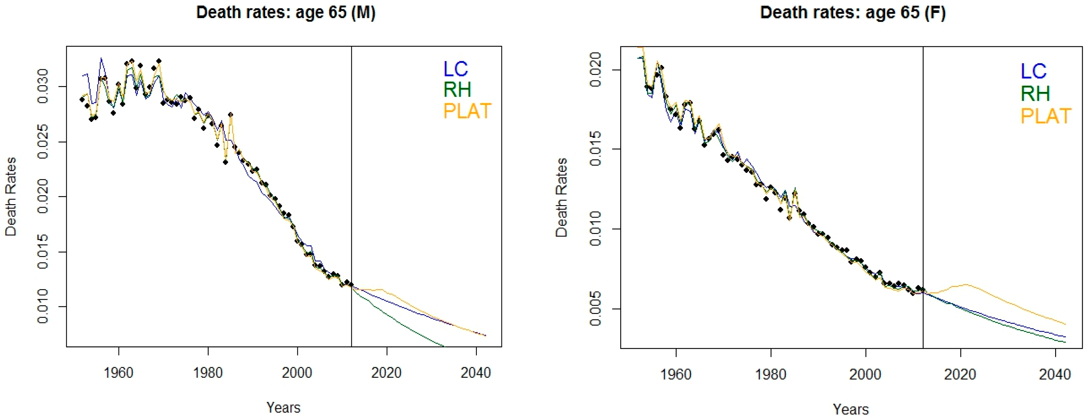
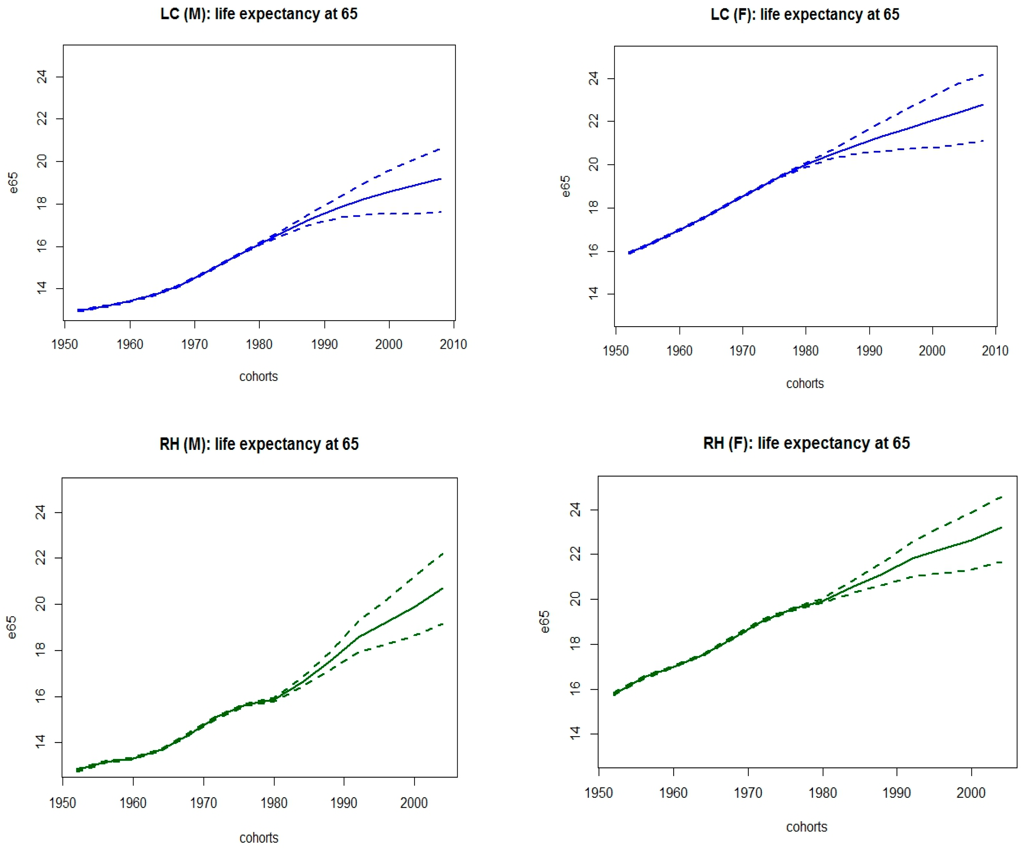
For each selected mortality model, the forecasting procedure for cohort effects ${\gamma }_{t-x}$ is based on the best ARIMA process fitting the observed data (Hyndman and Khandakar 2008). Figure 3 shows observed and fitted death rates, along with projections thirty years onwards; accordingly, Figure 2 displays the corresponding life expectancy at age 65 and their averaged version. Models have been assembled via a weighted sum of fitted central death rates and projections, considering the AIC weights reported in Table 1.

We notice that the assembling technique is able to balance the increase in life expectancy foreseen by the RH model with the results implied by the others and this circumstance is stronger for the male population.

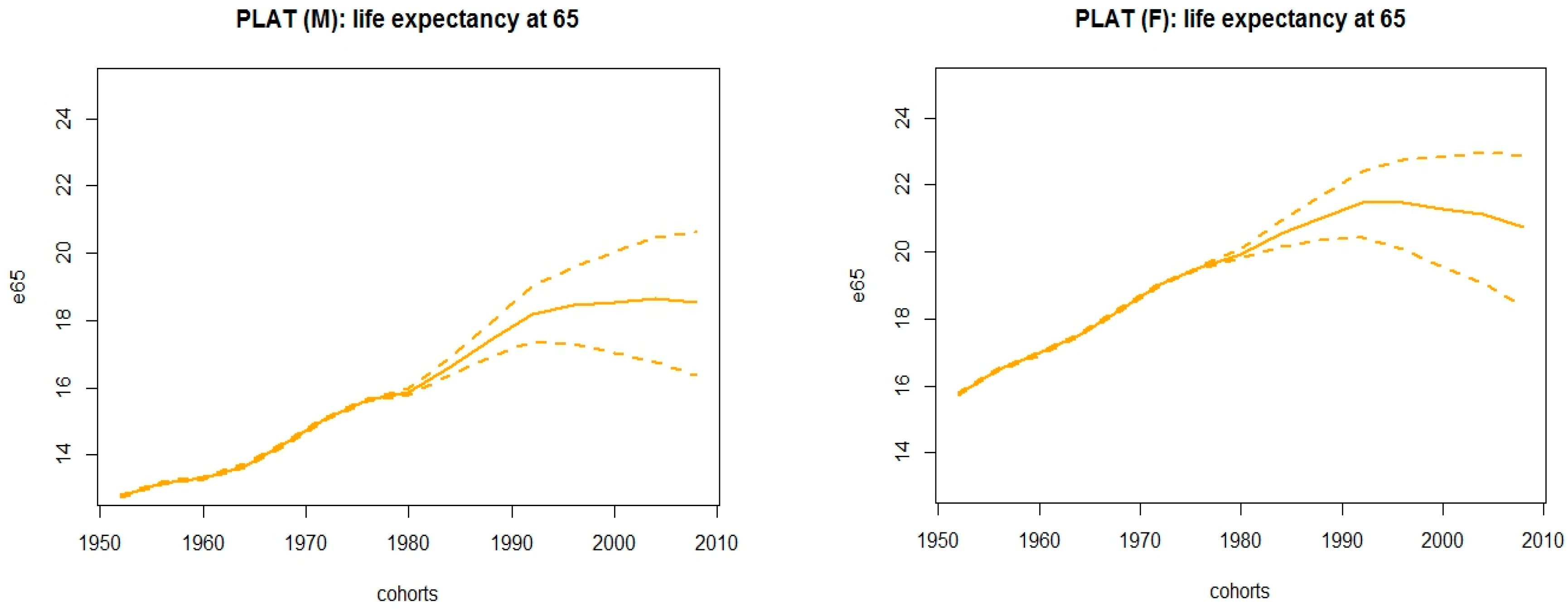
Interestingly, the best fitting Plat model foresees that life expectancy at 65 will be stationary around 18.5 (21) years for cohorts 1992 onwards for the male (female) population, with a slightly decreasing trend for females. As a consequence, the indexation mechanism reflects this circumstance for younger cohorts by implying a decay in the lag required to adjust the retirement age. This phenomenon could be explained by invoking the alleged narrowing in gender gap for the longevity risk, implied by the fact that the improvement in longevity is decelerating for women. On one hand, several studies have tried to answer to the question: Why women live longer than men? Finding answers in social behaviour and role, genetics, prevalence of cardio-vascular diseases for men, hormones and Darwinian perspective. On the other hand, recent findings highlight weaker improvements in longevity for women at older ages (that can be spotted already from Figure 1). Possible explanations for this phenomenon are to be found in closeness in reaching the maximum possible survivorship, worse mortality trends caused by lung cancers, improved health care for cardio-vascular diseases most occurring for men, among other factors (Sundberg et al. 2018; Ehiemua 2014). See also the comprehensive paper by Pattinson et al. (2012) and the international comparison therein. 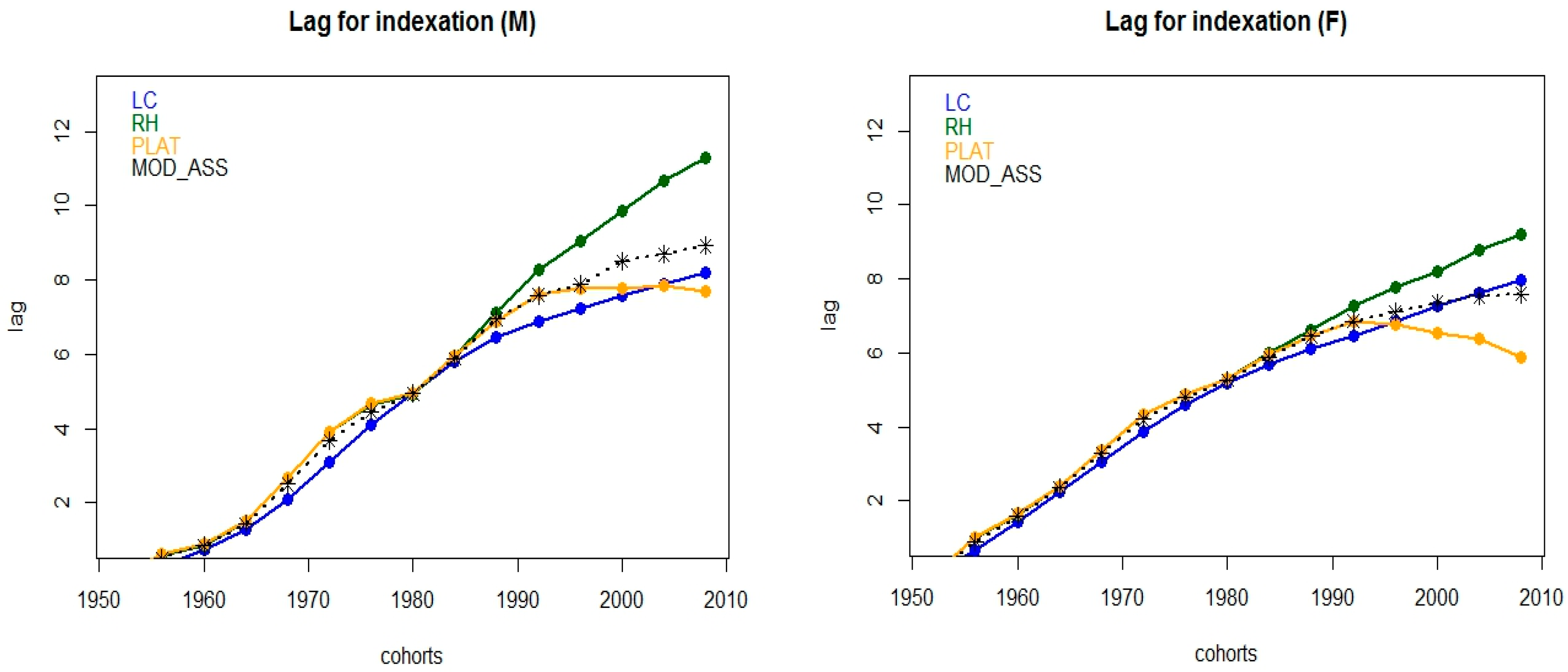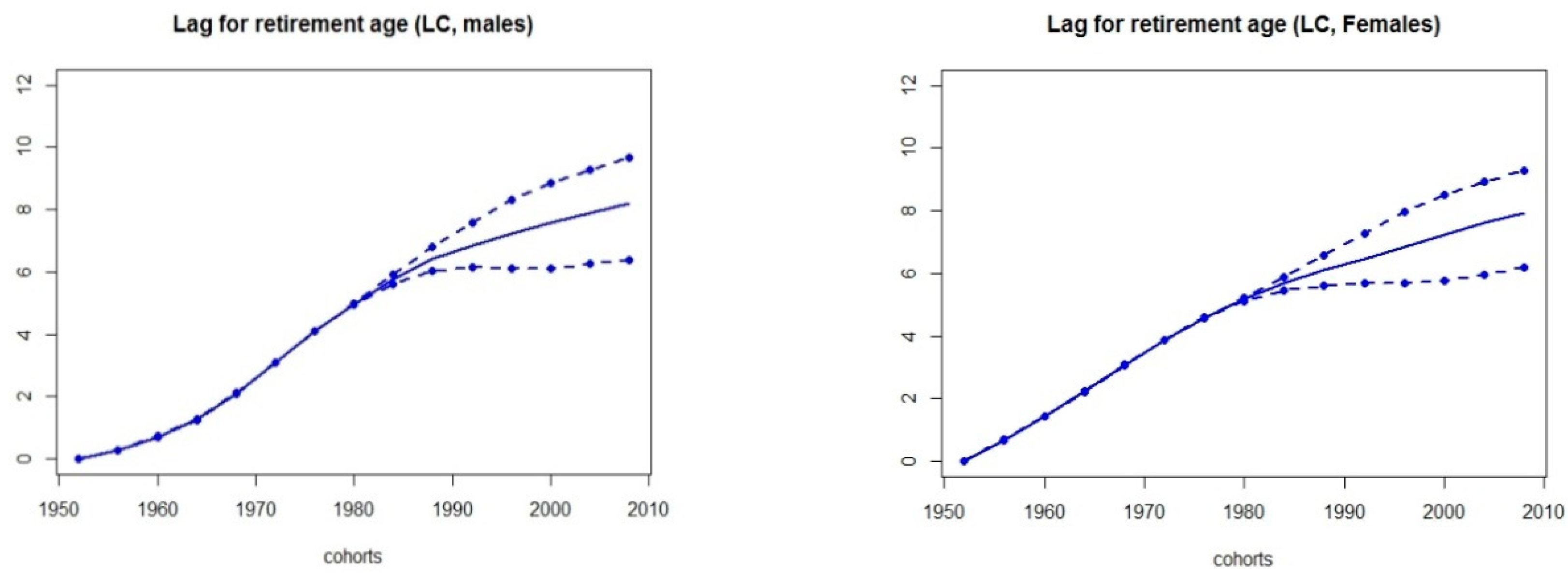Figure 4 displays the implied lag for indexation introduced in Section 2 for both the selected models and the assembled one, for all the cohorts in our study.

The mitigation effect implied by the model assembling technique is accounted also at the indexation step, where the forward shift for retirement age implied by the RH model is balanced out with those deriving by using the other models, thus yielding to a more feasible application of the flexible retirement scheme. In addition, the model assembling is advisable since its application trades off fitting and prediction capabilities.

In this regard, as mortality rates are projected with uncertainty, prediction intervals have to be associated to the future population at each age. In particular, since our analysis is concerned with older ages (ages greater than 65) and thus, only with a subsample of the whole population, parameter uncertainty needs to be incorporated in the modelling.

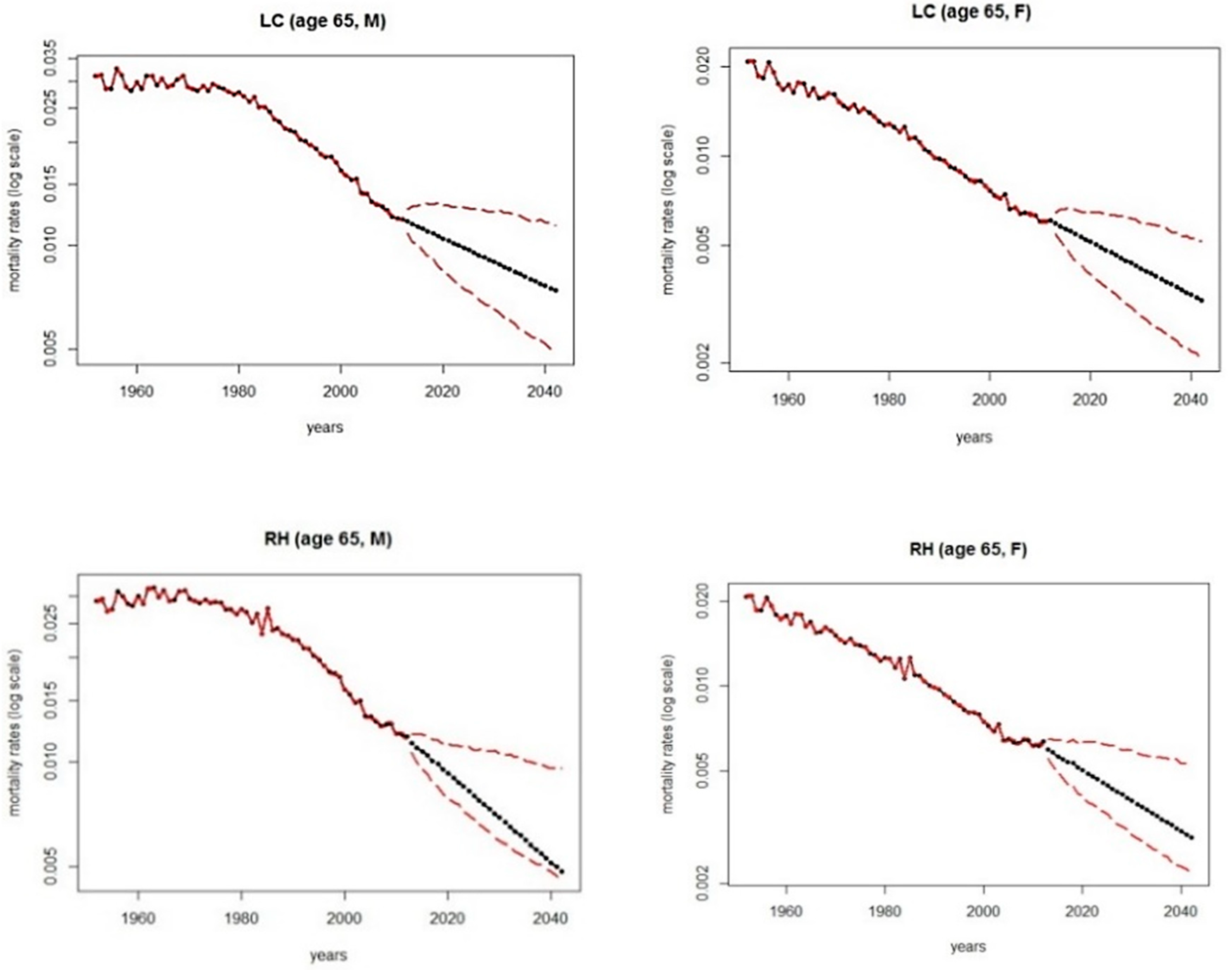
Figure 5 displays fitted and forecasted deaths rates (30 years ahead) according to the selected models (black solid lines): red dashed lines identify prediction intervals to account for uncertainty of parameter estimates and correspond to 5% bootstrap quantiles. Here we consider the semiparametric bootstrap proposed in Brouhns et al. (2005): thus, best and worst scenarios have been designed accordingly. Then, assuming the lower and upper bounds for prediction intervals of projection of mortality rates, Figure 6 and Figure 7 display expected life span and corresponding lags implied by the proposed indexation mechanism (solid lines), and in case the worst and best scenarios apply (dashed lines): right panels refer to males and left ones refer to females: d. Notice that here we assume the perspective of the National Security System and thus “worst” refers to the circumstance of the lower predictions for mortality rates and consequently higher life expectancy; dually, “best” refers to the circumstance of the highest predictions for mortality rates.

It might be argued that the flexible retirement approach here adopted could appear more applicable in terms of social implications if the EPPD would be re-evaluated over time to prevent from too high lags: for instance, the benchmark cohort could be updated at constant time intervals decided from the policymakers. In general, to smooth the impact of the shift on the retirement age, the longevity risk could be distributed and shared between the active and the retirement periods, for instance by halving the lag before applying the age shift. Nevertheless, the model assembling technique is a valuable data-driven tool to mitigate the shift of the retirement age, which could be too generous or too conservative if implied under a unique model, assuming thus a huge uncertainty risk.

In addition, it is worth to underline that the approach here presented is strictly actuarial and it advises gender-based time-shift for the retirement age to cope with different evolving paths in mortality rates. Historically, in Italy the retirement age has been different for men and women and for different work sectors. The Fornero Reform has completed a process of convergence towards a uniform age that had already begun for a long time. In 2018, the retirement age became 66 years and 7 months for both men and women. However, the aforementioned Reform also includes the so-called Early Retirement Pension (ERP). In that case a different treatment for men and women persists. In fact, ERP is due to men who have paid contributions for at least 42 years and 10 months and to women who have paid for at least 41 years and 10 months, regardless of age. Since any discrimination between men and women is forbidden in European Social Security Systems, to the practical extent our study could be applied considering the weighted average of the lags calculated for men and women, as it is done in UK and other countries for life expectancy (see for example DWP 2013), thus implying the same adjustment for the whole population.

5. Concluding Remarks

The paper is framed in the context of flexible pension schemes, which are developing in many countries in the last few years. We emphasize that our contribution to the current literature covers different topics. First of all, referring to the Italian population, we forecast mortality by using selected models within the GAPC family. Then, we consider an indexing mechanism based on the expected residual life to adjust the retirement age and keep a constant Expected Pension Period Duration. Thus, we support the idea of resorting to an indexed pension system that takes model risk into account. Indeed, acknowledging the gender gap in longevity and given evidence for its narrowing, the indexation mechanism and the application of the model assembling could help National Security System managements in coping with the longevity risk in practice.

In conclusion, notice that the background idea of the proposed indexation mechanism can be easily adapted to plan retirement strategies for younger cohorts. For instance, consider people aged 30 and calculate today the expected residual life $e_{30}$. If the retirement age were established by law at age $x_0$ (say, 65), then today one can establish that future pensions should be paid for an expected amount of years equal to 30 + $e_{30}$ − $x_0$. For a given stochastic mortality model, one could consider predicted death rates and, on that basis, assess $e_{x_0}$: longevity risk implies that one should expect $e_{x_0}>30 + e_{30} - x_0.$ Then, a flexible retirement scheme could be obtained to switch retirement age from $x_0$ to $x_0+\mathrm{lag}$ if:

$$\mathrm{lag}=\inf \left\{ j |e_{x_0+j}\le 30 + e_{30} - x_0\right\}$$

The benchmark pension duration $30 + e_{30} - x_0$ could be updated for each cohort or, as in the proposal of this contribution, could be set to that of a reference cohort. In order to keep the forecasted time span within reasonable values, one could consider people aged 30 in a past time period, for instance. This extension, as well as the inclusion of the financial risk within the flexible retirement mechanism, is under development.