Changes of Relation in Multi-Population Mortality Dependence: An Application of Threshold VECM

Abstract

Standardized longevity risk transfers often involve modeling mortality rates of multiple populations. Some researchers have found that mortality indexes of selected countries are cointegrated, meaning that a linear relationship exists between the indexes. Vector error correction model (VECM) was used to incorporate this relation, thereby forcing the mortality rates of multiple populations to revert to a long-run equilibrium. However, the long-run equilibrium may change over time. It is crucial to incorporate these changes such that mortality dependence is adequately modeled. In this paper, we develop a framework to examine the presence of equilibrium changes and to incorporate these changes into the mortality model. In particular, we focus on equilibrium changes caused by threshold effect, the phenomenon that mortality indexes alternate between different VECMs depending on the value of a threshold variable. Our framework comprises two steps. In the first step, a statistical test is performed to examine the presence of threshold effect in the VECM for multiple mortality indexes. In the second step, threshold vector error correction model (TVECM) is fitted to the mortality indexes and model adequacy is evaluated. We illustrate this framework with the mortality data of England and Wales (EW) and Canadian populations. We further apply the TVECM to forecast future mortalities and price an illustrative longevity bond with multivariate Wang transform. Our numerical results show that TVECM predicted much faster mortality improvement for EW and Canada than single-regime VECM and thus the incorporation of threshold effect significant increases longevity bond price.

1. Introduction

According to a recent report by World Health Organization (2015), global life expectancy raised dramatically from 64 years in 1990 to 71 years in 2013. The global aging trend is primarily attributed to greater consciousness of healthy lifestyles, development of new medicines, and improvement of health systems in many countries. Milidonis and Efthymiou (2017) identified causation from wealth to mortality improvement in Asia-Pacific countries and revealed that mortality improvements appear faster in more developed than less developed countries. Although increased life expectancy is desirable for individuals, this global trend poses significant financial burdens to social security systems, annuity providers, and pension plan sponsors. As a result, hedging of longevity risk has become an important issue which has attracted much discussion in recent years.

In general, longevity risk hedge can be categorized into customized hedge or standardized hedge. Examples of customized hedge include buy-in, buy-out, and customized longevity swap. Tailored to the hedger’s longevity exposure, customized hedge is effective in transferring longevity risk. However, customized hedge is very illiquid and has long maturity. Alternatively, standardized hedge links the payoff of longevity securities to a broad longevity index. It is more transparent and liquid, but less effective due to the difference between the population associated with the hedger’s longevity exposure and that underlying the longevity index. The first standardized longevity hedge, which took place in January 2008, is a q-forward contract written on mortality rates of 65-year-old males from England and Wales (EW) between J. P. Morgan and the U.K. pension fund buy-out company Lucida. More recently, Swiss Re launched the Kortis longevity bond to hedge the divergence in mortality improvement between EW and the United States.

Standardized longevity hedge often involves the mortality rates of multiple populations. For example, the Longevity Divergence Index of the Kortis bond depends on the mortality rates of male populations in both EW and the United States. Modeling the mortality dependence of the two populations is crucial for generating accurate forecasts of future Longevity Divergence Index values. The promotion of standardized longevity hedge in recent years has motivated research in multi-population mortality modeling. A comparative study of two-population mortality models can be found in Villegas et al. (2017).

Existing literature in multi-population mortality modeling is often built on the concept of coherence. Originally proposed by Li and Lee (2005), coherent mortality forecasting assumes that the relative mortality rates of any two related populations are mean-reverting; hence, coherent mortality forecasts do not diverge indefinitely over time. The model of Li and Lee (2005) has been adopted by several researchers, including Biffis et al. (2017), Li and Hardy (2011), and Milidonis et al. (2011). Other examples of coherent models include the two-population model proposed by Cairns et al. (2011), the gravity model by Dowd et al. (2011), and the application of vector error correction model (VECM) by Zhou et al. (2014).

Li et al. (2016) criticized that the hypothesis of coherence for being too strong and not always appropriate. A coherent multi-population mortality model may understate the range of possible mortality differentials between two populations. To address this problem, Li et al. (2016) proposed the concept of semicoherence, which is incorporated into mortality forecasts by using a three-regime threshold vector autoregression model. In the middle regime, where the mortality differential between populations does not exceed a specific tolerance corridor, the mortality trajectories of two related populations are allowed to diverge. In the lower and upper regimes, where the mortality differential exceeds the tolerance corridor, mean reversion comes into effect and brings the mortality differential back into the tolerance corridor.

Hunt and Blake (2015), after observing that the relative mortality rates appear to change over time, advocated against the imposing of coherence. They used the the cointegration technique to allow for covariation between mortality rates in the two populations. Cointegration and the resulted vector error correction model (VECM) was introduced by Engle and Granger (1987) to model the long-term tendency of cointegrated variables moving around common stochastic trends, i.e., the long-term equilibrium of cointegrated variables. VECM is essentially a special case of vector autoregressive (VAR) model. VECM has been used in mortality modeling by several other researchers including Kuo et al. (2003), Darkiewicz and Hoedemakers (2004), Lazar (2004), Gaille and Sherris (2011), Yang and Wang (2013), and Zhou et al. (2014).

The existence of cointegration relation has been confirmed among the mortalities of selected countries. The threshold behavior of the VAR model observed by Li et al. (2016) suggests that a fixed relation may be inappropriate for certain countries. However, no existing literature on mortality modeling has yet considered the possibility of changing cointegration relations over time. Changes in the cointegration relation may lead to significant adjustments in the mortality dependence. Therefore, it is essential to incorporate such changes in the multi-population mortality models. Although the threshold VAR used in Li et al. (2016) can accommodate changes in the VAR relation, it does not take cointegration or long-term equilibrium into account. In this paper, we improve on the threshold of Li et al. (2016) by considering threshold VECM (TVECM) proposed by Hansen and Seo (2002), which incorporates both threshold effect and cointegration relation.

In particular, we develop a framework to examine the presence of long-term relation changes and to incorporate these changes into the mortality model. We focus on the equilibrium changes caused by threshold effect, the phenomenon that mortality indexes alternate between different VECMs depending on the value of a threshold variable. We first perform a statistical test to examine the presence of threshold effect in the VECM for multiple mortality indexes. We then apply TVECM to model changes in the cointegration relation. The time series behavior is determined by whether the deviation from the long-term relation is above or below certain threshold values.

For illustrative purposes, we fitted the TVECM model to the mortality rates of EW and Canadian populations. Our statistical test suggests that the relation between EW and Canadian mortalities changes when the deviation from the long-term equilibrium exceeds or fall below certain threshold value; hence, the threshold effect exists. In addition, we used multivariate Wang transform to price an illustrative longevity bond and demonstrate that incorporating changes in the cointegration relation has a significant impact on longevity bond pricing.

The remainder of the paper is organized as follows: Section 2 introduces the dataset and the base mortality model. Section 3 detects and removes outliers in the mortality indexes. Section 4 performs cointegration analysis and estimates VECM. Section 5 introduces TVECM and its estimation. Section 6 applies TVECM in longevity bond pricing. Section 7 presents the conclusion.

2. The Base Mortality Model

2.1. The Lee–Carter Model

The Lee–Carter model, proposed in Lee and Carter (1992), is the most widely used mortality model. It has been recommended for use by the US Bureau of the Census as a benchmark model (Mitchell et al. 2013). The Lee–Carter model is expressed as:

$$\ln (m_{x,t}^{(i)})=a_x^{(i)}+b_x^{(i)}{k}_t^{(i)},$$

where $(i)$ represents the ith population; $m_{x,t}^{(i)}$ is the central mortality rate for a life aged x at time t from population $(i)$; $a_x^{(i)}$ represents the stand-alone age-specific parameters describing the average level of mortality at age x; $k_t^{(i)}$ referred to as mortality index, is the time-varying parameter which signifies the general speed of mortality improvement and captures the main time trend for all ages; and $b_x^{(i)}$ is the age-specific parameter that interacts with $k_t^{(i)}$.

Let $D_{x,t}^{(i)}$ and $E_{x,t}^{(i)}$ be the number of deaths and number of exposures-to-risk at age x in year t for population $(i)$. We assume that $D_{x,t}^{(i)}$ follows Poisson distribution with mean equal to $E_{x,t}^{(i)}{m}_{x,t}^{(i)}$. The loglikelihood for population $(i)$ can be written as

$$L{L}^{(i)}=\sum _{x,t}{D}_{x,t}^{(i)}ln{E}_{x,t}^{(i)}{m}_{x,t}^{(i)}-E_{x,t}^{(i)}{m}_{x,t}^{(i)}-ln(D_{x,t}^{(i)}!).$$

We maximize the log-likelihood to obtain the parameter estimates of $a_x^{(i)}$, $b_x^{(i)}$, and $k_t^{(i)}$ for each population. To obtain a unique set of parameter estimates, we impose two identification constraints: $\sum b_x^{(i)}=1$ and $\sum k_t^{(i)}=0$. Details of the model estimation method can be found in Brouhns et al. (2002). The model estimation can be performed in R using the “fit” function in the “StMoMo” package.

2.2. Data and Estimated Parameters

We used the mortality data of EW and Canadian populations aged 50–89 from 1922 to 2011.1 The mortality rates were acquired from Human Mortality Database (2017). We use Superscript (1) for EW and Superscript (2) for Canada in the mathematical expressions.

Parameter estimates of the Lee–Carter model of $a_x^{(i)}$ and $b_x^{(i)}$ are depicted in Figure 1. Figure 1a shows that both $a_x^{(1)}$ and $a_x^{(2)}$ increase steadily as the age rises, thus indicating that average mortality rates increase with age. $a_x^{(1)}$ is higher than $a_x^{(2)}$, thereby suggesting that EW population has overall higher mortality rate than Canadian population for the same age group. In Figure 1b, the decreasing trend of $b_x^{(i)}$ suggests that mortality rates at older ages are less sensitive to the changes in $k_t^{(i)}$.

Figure 1c plots the estimated time-varying parameters $k_t^{(1)}$ and $k_t^{(2)}$ from 1922 to 2011. Both $k_t^{(1)}$ and $k_t^{(2)}$ generally decline during this sample period, thus implying that mortality rates are decreasing in both regions. The trajectories of $k_t^{(1)}$ and $k_t^{(2)}$, which are very close, cross each other several times over the sample period. Therefore, it is necessary to investigate whether these trajectories share a common trend and to determine how they move around this trend.

3. Removing Additive Outliers

Figure 1c shows that the EW population had mortality rate spikes in 1931 due to the Great Depression, in 1941 due to World War II and, and in 1953 possibly due to the 1952 Great Smog of London. At the same time, members of the Canadian population were not or marginally affected by these one-time events. Outliers in the time series data may significantly affect model identification, estimation, and forecasting (Bovas and Box 1979; Chen and Tiao 1990). In our case, the outliers in $k_t^{(1)}$ may also distort the estimated relation between $k_t^{(1)}$ and $k_t^{(2)}$. Chen and Liu (1993) developed an iterative procedure to detect outliers in univariate time series data and obtain joint estimates of model parameters and outlier effects. In particular, four types of outliers were considered:

• Additive outlier, which causes an immediate and one-time effect on the observed series;
• Temporary change, which produces an initial effect that dies out gradually over time;
• Level shift, which produces an abrupt and permanent step change in the series; and
• Innovative outlier, which produces a temporary effect on stationary time series, but will gradually converge to a permanent effect on non-stationary time series.

For more details about this procedure, readers are advised to read Chen and Liu (1993).

Here, we considered removing only additive outliers, because other types of outliers have impact on mortality for multiple years and may still contain useful information about the relation between the two populations. We used the “tso” function in the “tsoutlier” R package to identify and remove additive outliers with the critical value of 3.5 as the criterion for the determination of outliers. The detected additive outliers are shown in

Table 1. Detected additive outliers in the time-varying parameter series.

Population	Type	Year	t-Value
EW	Additive Outlier	1931	3.54
	Additive Outlier	1942	7.61
	Additive Outlier	1953	4.58
Canada	None

. Additive outliers only present in $k_t^{(1)}$. The original and outlier-adjusted $k_t^{(1)}$ series are displayed in Figure 2. In the following analysis, $k_t^{(1)}$ represents outlier-adjusted $k_t^{(1)}$ data if not stated.

4. Vector Error Correction Model

4.1. Cointegration

Cointegration is an economic concept that mimics the existence of a long-term equilibrium among an economic time series. A time series $y_t$ is integrated ($I(1)$) if its first difference $\Delta y_t=y_t-y_{t-1}$ is stationary ($I(0)$). If two or more integrated time series have a stationary linear combination, then they are cointegrated. In particular, $k_t^{(1)}$ and $k_t^{(2)}$ are cointegrated if

• $k_t^{(1)}$ and $k_t^{(2)}$ are both $I(1)$ variables; and
• there exists a linear combination with a constant $\beta$ and $\beta \ne 0$ such that

  $$k_t^{(1)}+\beta k_t^{(2)}\sim \mathit{I}(0).$$

When $k_t^{(1)}$ and $k_t^{(2)}$ are cointegrated, they are driven by a common trend and the variations of the two variables are correlated.

4.2. VECM Model

VECM is a special case of vector autoregressive (VAR) model with cointegration relationship taken into consideration. A VAR model with lag order p can be written as

$$\left(\begin{array}{c}{k}_t^{(1)}\\ k_t^{(2)}\end{array}\right)=c+\sum _{i=1}^p{\mathrm{\Phi }}_i\left(\begin{array}{c}{k}_{t-i}^{(1)}\\ k_{t-i}^{(2)}\end{array}\right)+\left(\begin{array}{c}{\epsilon }_t^{(1)}\\ {\epsilon }_t^{(2)}\end{array}\right),$$

where c is a $2\times 1$ constant vector, ${\mathrm{\Phi }}_i$ is a $2\times 2$ loading matrix for lag i, and $\left(\begin{array}{c}{\epsilon }_t^{(1)}\\ {\epsilon }_t^{(2)}\end{array}\right)$ follows bivariate normal distribution.

A p-order VAR can be written as a $(p-1)$-order VECM, as shown below:

$$\left(\begin{array}{c}\Delta k_t^{(1)}\\ \Delta k_t^{(2)}\end{array}\right)=c+\mathrm{\Pi }\left(\begin{array}{c}{k}_{t-1}^{(1)}\\ k_{t-1}^{(2)}\end{array}\right)+\sum _{i=1}^{p-1}{\mathrm{\Gamma }}_i\left(\begin{array}{c}\Delta k_{t-i}^{(1)}\\ \Delta k_{t-i}^{(2)}\end{array}\right)+\left(\begin{array}{c}{\epsilon }_t^{(1)}\\ {\epsilon }_t^{(2)}\end{array}\right),$$

where $\mathrm{\Pi }$ is a $2\times 2$ long-term loading matrix and ${\mathrm{\Gamma }}_i$ is a $2\times 2$ short-term loading matrix for lag i.

The rank of $\mathrm{\Pi }$ indicates whether $k_t^{(1)}$ and $k_t^{(2)}$ have a cointegration relationship. If the rank of $\mathrm{\Pi }$ is 0, then there is no long-term equilibrium and the differenced $k_t^{(i)}$ series are stationary. If the rank of $\mathrm{\Pi }$ is full, then the original time series $k_t^{(i)}$ must be stationary. Otherwise, $k_t^{(1)}$ and $k_t^{(2)}$ are cointegrated. Since we only have two time series in our study, the full rank is 2. Cointegration relationship exists only when the rank of $\mathrm{\Pi }$ is equal to 1. In the case that cointegration exists, VECM can be rewritten as follows:

$$\left(\begin{array}{c}\Delta k_t^{(1)}\\ \Delta k_t^{(2)}\end{array}\right)=c+\alpha \left(k_{t-1}^{(1)}+\beta k_{t-1}^{(2)}\right)+\sum _{i=1}^{p-1}{\mathrm{\Gamma }}_i\left(\begin{array}{c}\Delta k_{t-i}^{(1)}\\ \Delta k_{t-i}^{(2)}\end{array}\right)+\left(\begin{array}{c}{\epsilon }_t^{(1)}\\ {\epsilon }_t^{(2)}\end{array}\right),$$

where $\alpha$ is the $2\times 1$ adjustment coefficient vector and $\beta$ is the cointegrating value. VECM incorporates both the long-term equilibrium relationship and the short-term relationship. In the long run, the two time series are expected to follow the relationship $k_t^{(1)}+\beta k_t^{(2)}=0$. If there is deviation from this equilibrium, the error correction term $\alpha (k_t^{(1)}+\beta k_t^{(2)})$ pulls the time series towards the equilibrium. In the short-term, the two time series are affected by their autoregressive terms. We can also allow constant and time trend in the cointegration term. However, we find that these terms are not necessary for our dataset during the process of model building described in the following section.

4.3. Model Building

We used the following procedures to build and estimate VECM:

• Test if $k_t^{(1)}$ and $k_t^{(2)}$ follow $I(1)$ process.
• Determine the lag order of VECM.
• Perform cointegration tests to examine if a cointegration relationship exists.
• Estimate the VECM with selected lag order.
• Check residual diagnostics.

We used the Augmented Dickey–Fuller (ADF) test to check whether the two time series are $I(1)$ processes. The null hypothesis of ADF test is that unit roots exist. The existence of unit roots indicates that the tested time series is non-stationary. We expect that the null hypothesis is accepted for the original $I(1)$ process and rejected for the first-order difference of the $I(1)$ process. In other words, we expect $k_t^{(1)}$ and $k_t^{(2)}$ to be non-stationary processes but their first-order differences to be stationary.

Table 2. Augmented Dickey–Fuller test results.

Data	Test Statistic	p-Value
$k_t^{(1)}$	3.81	>10%
$k_t^{(2)}$	3.44	>10%
$\Delta k_t^{(1)}$	−8.83	<1%
$\Delta k_t^{(2)}$	−8.15	<1%

summarizes the ADF test results for $k_t^{(1)}$, $k_t^{(2)}$, $\Delta k_t^{(1)}$, and $\Delta k_t^{(2)}$. The tests include a drift and use Akaike Information Criteria to select lag order in the test regression. The test statistics for both $k_t^{(1)}$ and $k_t^{(2)}$ have p-value greater than 10%, indicating that we cannot reject the null hypothesis that $k_t^{(1)}$ and $k_t^{(2)}$ are non-stationary at 10% significance level. The test statistics for $\Delta k_t^{(1)}$ and $\Delta k_t^{(2)}$ are both smaller than 1%, suggesting that we reject the null hypothesis at 1% significance level. Therefore, both $\Delta k_t^{(1)}$ and $\Delta k_t^{(2)}$ are stationary. According to the definition of $I(1)$ process, we can conclude that both $k_t^{(1)}$ and $k_t^{(2)}$ are $I(1)$ processes.

To select the lag order for VECM, we first determine the lag order for VAR, and then deduct the order by one for VECM. In the lag order selection for VAR, we consider two criteria: Akaike Information Criteria (AIC), and Bayes Information Criteria (BIC). Since the VAR models are estimated by Ordinary Least Square (OLS) method, AIC and BIC are calculated using the following equations:

$$\begin{array}{ccc}\hfill \mathrm{AIC}& =& \ln \left|\frac{1}{T}\sum _{t=1}^T{\epsilon }_t{\epsilon }_t^{\prime }\right|+\frac{2}{T}p{K}^2,\hfill \\ \hfill \mathrm{BIC}& =& \ln \left|\frac{1}{T}\sum _{t=1}^T{\epsilon }_t{\epsilon }_t^{\prime }\right|+\frac{ln(T)}{T}p{K}^2\hfill \end{array}$$

where ${\epsilon }_t={[{\epsilon }_t^{(1)},{\epsilon }_t^{(2)}]}^{\prime }$, $\left|X\right|$ denotes the determinant of a matrix X, T is the sample size, p is the lag order, and K is the dimension of the time series data. The lower the criteria values, the better the goodness of fit.

Table 3. Lag order selection for VAR model.

Criteria	Lag Order
	1	2	3	4	5
AIC	−0.04	−0.53	−0.57	−0.58	−0.52
BIC	0.13	−0.24	−0.17	−0.07	0.11

shows that lag order 4 has the lowest AIC, while lag order 2 has the lowest BIC. The two criteria lead to different conclusions since they penalize extra parameters to different extents. It is often believed that AIC selects the model that most adequately describes the data and BIC tries to find the true model among the set of candidates. As a result, the model selected by AIC tends to overfit while the one selected by BIC may underfit. We fit both VECM(1) and VECM(3) one lag less than the corresponding VAR model, and check residual diagnostics to select an adequate model.

Next, we test whether $k_t^{(1)}$ and $k_t^{(2)}$ are cointegrated using the Engle–Granger test. We first perform a linear regression of $k_t^{(1)}$ on $k_t^{(2)}$, and then conduct ADF test on the regression residuals. The estimated linear regression model is shown below:

$$k_t^{(1)}=\underset{(0.1959)}{-0.1574}+\underset{(0.0159)}{0.9863}{k}_t^{(2)},$$

where the numbers in parentheses are the standard deviations of the estimated parameters. The ADF test on the regression residuals returns a p-value smaller than 5%, indicating that we reject the null hypothesis of the existence of unit roots at 5% significance level. Therefore, the regression residuals are stationary and $k_t^{(1)}$ and $k_t^{(2)}$ are cointegrated. Since the constant term in the regression model is insignificant, we choose not to include a constant in the cointegration term.

Finally, VECM is estimated by the Engle–Granger two-step ordinary least squares (OLS). The estimation can be conducted in R using the “VECM” function in the “tsDyn” package. The first OLS determines the cointegrating value $\beta$ by a linear regression of $k_t^{(1)}$ on $k_t^{(2)}$, which has been carried out in the cointegration test. Conditioning on the estimated $\beta$, the second OLS is performed to obtain other parameters in VECM. VECM can also be estimated by a one-step maximum likelihood estimation (MLE) method. However, in our case, the MLE estimates are very unstable when we use different number of lag orders.

Since AIC and BIC suggest different lag orders, we fit both VECM(1) and VECM(3) and examine the adequacy of the estimated models.

Table 4. p-values of Ljung–Box autocorrelation test for VECM.

Model	Lag Order
	2	4	6	8	10
VECM(1)	0.95	0.21	0.15	0.16	0.12
VECM(3)	0.97	0.30	0.26	0.16	0.20

presents the results of Ljung–Box autocorrelation test for VECM(1) and VECM(3). The p-values for both VECM(1) and VECM(3) are all significantly greater than 5%, thereby indicating autocorrelation has been properly captured by the two models.

Table 5. p-values of Doornick–Hansen normality test.

Model	Bivariate	Univariate
		(1)	(2)
VECM(1)	0.03	0.62	0.01
VECM(3)	0.28	0.68	0.12

presents the results of univariate and bivariate Doornick–Hansen (DH) normality test for the residuals from VECM(1) and VECM(3). Residuals from VECM(1) fails the bivariate normality test and also the univariate normality test for $k_t^{(2)}$ at 5% significance level. In contrast, residuals from VECM(3) pass all the normality test at 5% significance level. Overall, the residual diagnostics suggest that VECM(3) is more adequate than VECM(1) for our data. Therefore, we use VECM(3) in the following analysis.

The estimated VECM(3) is shown below:

$$\begin{array}{cc}\hfill \left(\begin{array}{c}\Delta k_t^{(1)}\\ \Delta k_t^{(2)}\end{array}\right)& =\left(\begin{array}{c}-0.7820\\ -0.4041\end{array}\right)+\left(\begin{array}{c}-0.0781\\ 0.0711\end{array}\right)\left(k_{t-1}^{(1)}-0.9862k_{t-1}^{(2)}\right)\hfill \\ & +\left(\begin{array}{cc}-0.6308& 0.2571\\ 0.0617& -0.1474\end{array}\right)\left(\begin{array}{c}\Delta k_{t-1}^{(1)}\\ \Delta k_{t-1}^{(2)}\end{array}\right)\hfill \\ & +\left(\begin{array}{cc}-0.0952& 0.0230\\ 0.1046& -0.0873\end{array}\right)\left(\begin{array}{c}\Delta k_{t-2}^{(1)}\\ \Delta k_{t-2}^{(2)}\end{array}\right)\hfill \\ & +\left(\begin{array}{cc}-0.0136& 0.0425\\ -0.0468& 0.2245\end{array}\right)\left(\begin{array}{c}\Delta k_{t-3}^{(1)}\\ \Delta k_{t-3}^{(2)}\end{array}\right)+\left(\begin{array}{c}{\epsilon }_t^{(1)}\\ {\epsilon }_t^{(2)}\end{array}\right).\hfill \end{array}$$

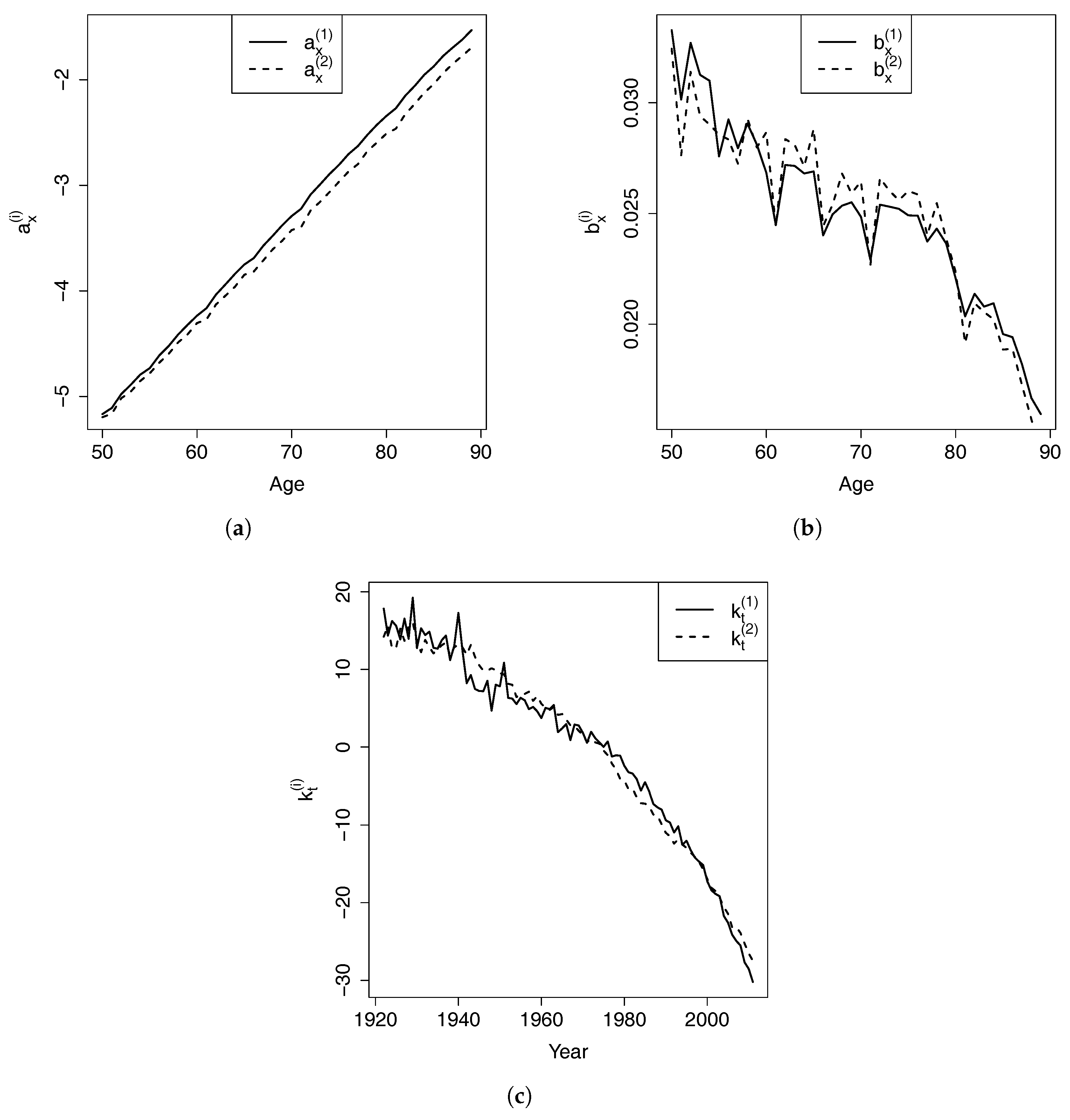
The estimated long-term equilibrium is $k_{t-1}^{(1)}-0.9862k_{t-1}^{(2)}=0$. The cointegrating value is close to −1, thereby indicating that $k_t^{(1)}$ and $k_t^{(2)}$ are close. However, because of the downward trend in the mortality indexes, the gap between $k_t^{(1)}$ and $k_t^{(2)}$ enlarges over time and $k_t^{(1)}$ and $k_t^{(2)}$ diverge slowly and indefinitely.

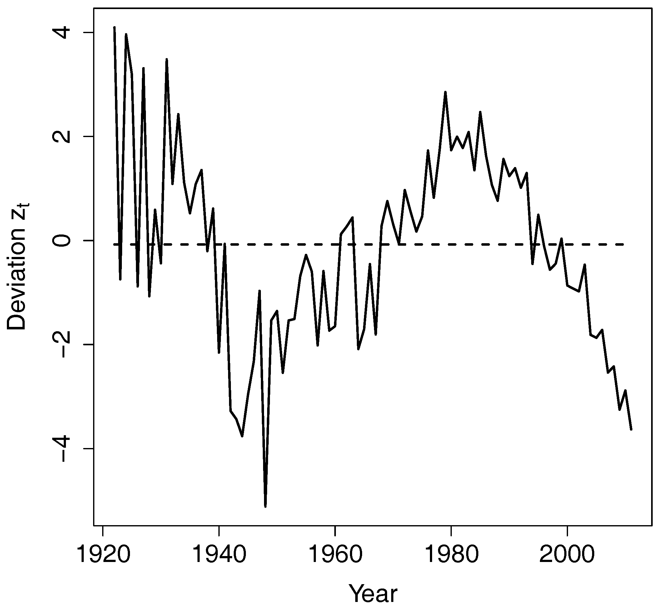
When $k_{t-1}^{(1)}$ is larger than $0.9862k_{t-1}^{(2)}$ in year $t-1$, the deviation from the equilibrium is positive. This deviation is multiplied by $-0.0781$ for $\Delta k_t^{(1)}$ and $0.0711$ for $\Delta k_t^{(2)}$, resulting in a reduction of $\Delta k_t^{(1)}$ and increase of $\Delta k_t^{(2)}$ in year t. Therefore, the expected difference between $k_t^{(1)}$ and $0.9862k_t^{(2)}$ in year t narrows. This is how the error correction term forces the two time series to revert to the long-term equilibrium.

5. Threshold Vector Error Correction Model

5.1. TVECM Model

Li et al. (2016) found threshold behavior when modeling multi-population mortality by VAR model, i.e., the time series data follow different VAR models depending on the value of a threshold variable. Since VECM is a special case of VAR model, we are interested in whether threshold effect also presents in VECM and how to incorporate the threshold effect by the threshold VECM (TVEM) model. The difference between TVECM and threshold VAR (TVAR) is that TVECM takes into account cointegration and hence an explicit long-term relation. Although the TVAR model used in Li et al. (2016) implies a mean-reverting mechanism, there is no explicit long-term relation.

Consider a two-regime TVECM in which the threshold variable is the deviation from the long-term equilibrium. Depending on whether the threshold variable exceeds the threshold value, VECM parameters may take different values. This TVECM can be expressed as:

$$\begin{array}{ccc}& \left(\begin{array}{c}\Delta k_t^{(1)}\\ \Delta k_t^{(2)}\end{array}\right)=\hfill & \hfill \left\{\begin{array}{c}{c}_1+{\alpha }_1\left(k_{t-1}^{(1)}+\beta k_{t-1}^{(2)}\right)+\sum _{i=1}^{p-1}{\mathrm{\Gamma }}_{1,i}\left(\begin{array}{c}\Delta k_{t-i}^{(1)}\\ \Delta k_{t-i}^{(2)}\end{array}\right)+\left(\begin{array}{c}{\epsilon }_t^{(1)}\\ {\epsilon }_t^{(2)}\end{array}\right),z_{t-1}>\gamma \hfill \\ c_2+{\alpha }_2\left(k_{t-1}^{(1)}+\beta k_{t-1}^{(2)}\right)+\sum _{i=1}^{p-1}{\mathrm{\Gamma }}_{2,i}\left(\begin{array}{c}\Delta k_{t-i}^{(1)}\\ \Delta k_{t-i}^{(2)}\end{array}\right)+\left(\begin{array}{c}{\epsilon }_t^{(1)}\\ {\epsilon }_t^{(2)}\end{array}\right),z_{t-1}\le \gamma \hfill \end{array}\right.\end{array}$$

where $c_n$ is the constant vector for regime n; ${\alpha }_n$ is adjustment coefficient vector for regime n; $\beta$ is cointegrating value; ${\mathrm{\Gamma }}_{n,i}$ is the AR coefficient for regime n and lag i; $z_{t-1}=k_{t-1}^{(1)}+\beta k_{t-1}^{(2)}$ measures the deviation from the long-term equilibrium; and $\gamma$ is the threshold value.

Which regime the time series lies in at time t depends on the value of $z_{t-1}$. If $z_{t-1}$ is higher than the threshold value $\gamma$, then the time series switches to the first regime at time t. If $z_{t-1}$ is lower than $\gamma$, then it switches to the second regime at time t. When there are more than two regimes, this expression can be easily extended. It is often assumed that there are one or two threshold values for model parsimony corresponding to two or three regimes, respectively.

5.2. Threshold Effect and Model Estimation

We fit the estimated $\{k_t^{(1)},k_t^{(2)}\}$ by a two-regime TVECM. We do not consider TVECM with higher regimes due to the consideration of model parsimony. The estimation of TVECM model is achieved by minimizing the residual sum of squares using a two-dimensional grid search on $\beta$ and $\gamma$. The estimation can be performed in R using the “TVECM” function in the “tsDyn” package. The estimated model is shown below:

$$\begin{array}{cc}\hfill \left(\begin{array}{c}\Delta k_t^{(1)}\\ \Delta k_t^{(2)}\end{array}\right)& =\left(\begin{array}{c}-1.3482\\ -0.8089\end{array}\right)+\left(\begin{array}{c}-0.3737\\ 0.2631\end{array}\right)z_{t-1}\hfill \\ & +\left(\begin{array}{cc}-0.4041& -0.4338\\ 0.0890& -0.2212\end{array}\right)\left(\begin{array}{c}\Delta k_{t-1}^{(1)}\\ \Delta k_{t-1}^{(2)}\end{array}\right)\hfill \\ & +\left(\begin{array}{cc}-0.3235& -0.3778\\ -0.0629& -0.1135\end{array}\right)\left(\begin{array}{c}\Delta k_{t-2}^{(1)}\\ \Delta k_{t-2}^{(2)}\end{array}\right)\hfill \\ & +\left(\begin{array}{cc}-0.3580& -0.4661\\ -0.2245& 0.3769\end{array}\right)\left(\begin{array}{c}\Delta k_{t-3}^{(1)}\\ \Delta k_{t-3}^{(2)}\end{array}\right)+\left(\begin{array}{c}{\epsilon }_t^{(1)}\\ {\epsilon }_t^{(2)}\end{array}\right),z_{t-1}>-0.0754\hfill \end{array}$$

$$\begin{array}{cc}\hfill \left(\begin{array}{c}\Delta k_t^{(1)}\\ \Delta k_t^{(2)}\end{array}\right)& =\left(\begin{array}{c}0.0354\\ -0.2738\end{array}\right)+\left(\begin{array}{c}0.0244\\ 0.0518\end{array}\right)z_{t-1}\hfill \\ & +\left(\begin{array}{cc}-0.5945& 0.4531\\ 0.0768& -0.1493\end{array}\right)\left(\begin{array}{c}\Delta k_{t-1}^{(1)}\\ \Delta k_{t-1}^{(2)}\end{array}\right)\hfill \\ & +\left(\begin{array}{cc}-0.0602& 0.5960\\ 0.2504& -0.0170\end{array}\right)\left(\begin{array}{c}\Delta k_{t-2}^{(1)}\\ \Delta k_{t-2}^{(2)}\end{array}\right)\hfill \\ & +\left(\begin{array}{cc}0.1456& 0.3559\\ 0.1018& 0.0535\end{array}\right)\left(\begin{array}{c}\Delta k_{t-3}^{(1)}\\ \Delta k_{t-3}^{(2)}\end{array}\right)+\left(\begin{array}{c}{\epsilon }_t^{(1)}\\ {\epsilon }_t^{(2)}\end{array}\right),z_{t-1}\le -0.0754\hfill \end{array}$$

where $z_t=k_t^{(1)}-0.9667k_t^{(2)}$, and the estimated variance-covariance matrix for the error term is $\left(\begin{array}{cc}1.0042& 0.2562\\ 0.2562& 0.4512\end{array}\right)$.

Before we apply the estimated TVECM, it is important to verify whether the threshold effect is significant in the dataset. We follow Hansen and Seo (2002) and test the presence of threshold effect in $\{k_t^{(1)},k_t^{(2)}\}$ based on the Lagrange multiplier principle. Asymptotic critical values and p-values of this test are calculated using fixed regressor bootstraps. Under the null hypothesis, there is no threshold effect, so the model reduces to a conventional VECM. Under the alternative hypothesis, the time series data follow a two-regime TVECM. This test can be implemented in R using the “TVECM.SeoTest” function in the “tsDyn” package. Given the cointegrating value of 0.9667, the p-value of the threshold effect test is 0.0272, thereby rejecting the null hypothesis of no threshold effect at 5% significance level.

Since VECM and TVECM are nested models, we also perform a likelihood ratio test to compare their goodness of fit. The test statistics is $2\times$ (loglikelihood of TVECM − loglikelihood of VECM), equal to $2(-37.7441+59.7507)$. The degree of freedom is (number of parameters in TVECM − number of parameters in VECM), equal to $(34-17)$. The p-value of the likelihood ratio test is 0.0003, thereby suggesting that TVECM provides significant improvement over VECM.

As we can see from the estimated model, the threshold value is estimated to be $-0.0754$ and the long-term equilibrium is $k_t^{(1)}-0.9667k_t^{(2)}=0$. When the deviation is higher than $-0.0754$, the corresponding adjustment coefficient vector is $\left(\begin{array}{c}-0.3737\\ 0.2631\end{array}\right)$. If the deviation is below $-0.7654$, then the corresponding adjustment coefficient vector is $\left(\begin{array}{c}0.0244\\ 0.0518\end{array}\right)$.

To understand how error correction works in the TVECM, we consider three cases:

• Case 1: $z_{t-1}>0$. The time series data are in the upper regime. $k_{t-1}^{(1)}$ is higher than it should be in the long-term equilibrium. Multiplying the deviation by the negative coefficient $-0.3737$ for EW pulls down $k_t^{(1)}$. At the same time, multiplying the deviation by the positive coefficient 0.2631 for Canada pulls up $k_t^{(2)}$. This adjustment brings $k_t^{(1)}$ and $k_t^{(2)}$ closer to their long-term equilibrium.
• Case 2: $-0.0754<z_{t-1}\le 0$. The time series data are still in the upper regime, but $k_{t-1}^{(1)}$ is lower than it should be in the long-term equilibrium. The deviation is multiplied by $-0.3737$ for EW and $0.2631$ for Canada, thereby pulling $k_t^{(1)}$ up and $k_t^{(2)}$ down. The error correction term narrows the deviation again and brings the time series towards their long-term equilibrium.
• Case 3: $z_{t-1}\le -0.0754$. The process is in the second regime and $k_{t-1}^{(1)}$ is lower than it should be in the long-term equilibrium. The negative deviation is multiplied by $0.0244$ for EW and 0.0518 for Canada, thereby pulling both $k_t^{(1)}$ and $k_t^{(2)}$ down. However, $k_t^{(1)}$ is pulled down to a smaller extent which results in a smaller deviation from the long-term equilibrium.

Figure 3 presents the historical process of the deviation $z_t$ in a solid line and the threshold value in a dashed line. During the periods of 1922 to 1940 and 1970 to 1995, the deviation is mostly greater than the threshold value. This indicates that the process is in the upper regime. During 1940–1970 and 1995–2011, the deviation is mostly smaller than the threshold value and hence the process is in the lower regime.

Based on the estimated TVECM model, the reversion to the long-term equilibrium is much faster in the upper regime than it is in the lower regime. Therefore, when experiencing higher mortality than that suggested by the long-term equilibrium, EW population improves their mortality at a faster rate, compared to the Canadian population. Causality analysis employed in Milidonis and Efthymiou (2017) may be used to study the causes of the difference between mortality improvement in the two populations.

Finally, we examine the autocorrelation and normality of the residuals obtained from TVECM.

Table 6. p-values of Ljung–Box autocorrelation test for TVECM.

Model	Lag Order
	2	4	6	8	10
TVECM	0.98	0.76	0.45	0.33	0.25

shows the result of the Ljung–Box autocorrelation test. The p-values for all the lag orders examined are greater than 5%, thereby indicating no significant autocorrelation in the residuals. We again perform the univariate and multivariate Doornick–Hansen normality test for the residuals. Test results are shown in

Table 7. p-values of Doornick–Hansen normality test for TVECM.

Model	Multivariate	Univariate
		(1)	(2)
TVECM	0.75	0.59	0.66

. Both multivariate test and univariate test for the residuals pass the normality test at 5% significance level.

5.3. Comparing Mortality Forecasts of VECM and TVECM

We simulate the paths of $k_t^{(1)}$ and $k_t^{(2)}$ from year 2012 to 2031 based on the estimated VECM and TVECM model, and determine the 95% prediction intervals. The simulation procedures are shown as follows:

• Let $t=2012$. Generate 5000 bivariate normal random vectors as the simulated error terms $\{{\epsilon }_t^{(1)},{\epsilon }_t^{(2)}\}$.
• Calculate the values of $k_t^{(1)}$ and $k_t^{(2)}$ based on the simulated errors for $t=2012$.
• Repeat Steps (1) and (2) for $t=2013,2014,\dots ,2031$.

Figure 4a compares the forecasts of $k_t^{(1)}$ obtained from VECM and TVECM. The mean forecasts of $k_t^{(1)}$ using the two models are close from 2012 to 2018, but gradually diverge afterwards. The forecasts from TVECM become lower than those from VECM as the forecast period increases. The prediction interval of TVECM is also smaller than that of VECM, because TVECM explains more variation in the data and hence yields residuals with smaller variance. Figure 4b compares the forecasts of $k_t^{(2)}$ using VECM and TVECM. We again observe that the forecasts of $k_t^{(2)}$ from TVECM are much lower than those from VECM. The prediction interval of TVECM is slightly smaller than that of VECM. Overall, we find that TVECM predicts much faster mortality improvement than VECM for both populations. The mortality improvement pattern predicted by TVECM appears to be more in line with which has been observed in recent years.

6. Pricing Longevity Bond

6.1. An Illustrative Longevity Bond

In this section, we price an illustrative longevity bond that hedges unexpected mortality improvement associated with EW and Canadian populations. Assume that this bond is issued at the end of 2011 and matures at the end of 2019. The bond issuer has annuity policies in both EW and Canada and annuitants are between age 75 and 85 at the beginning of 2012.

The longevity bond is traded at its face value. It pays quarterly coupon at three-month London Interbank Offered Rate (LIBOR) plus a spread. When the bond matures, the principal will be returned but may be subject to erosion. The principal repayment is associated with the mortality improvement of EW and Canada populations.

Let ${\mathrm{Improvement}}_x^{(i)}$ be the annual mortality improvement for an individual aged x from population $(i)$. It is defined as

$${\mathrm{Improvement}}_x^{(i)}=1-{\left(\frac{m_{x,2019}^{(i)}}{m_{x,2011}^{(i)}}\right)}^{1/8}.$$

The mortality improvement index for population $(i)$ is then defined as

$$\begin{array}{ccc}\hfill M{I}^{(i)}& =& \frac{1}{11}\sum _{x=75}^{85}{\mathrm{Improvement}}_x^{(i)}.\hfill \end{array}$$

The payment of the bond is linked to the weighted average of the mortality improvement (WMI) of the two populations. It is expressed as:

$$WMI=0.625M{I}^{(1)}+0.375M{I}^{(2)}.$$

We set the respective weights of $M{I}^{(1)}$ and $M{I}^{(2)}$ at 0.625 and 0.375, because Canadian population size is approximately 60% of EW population size. The principal of the bond is reduced if the realized mortality improvement is higher than a certain threshold value, thereby providing hedge for longevity risk. More specifically, the principal is reduced by a “principal reduction factor” ($PRF$) given below:

$$PRF=\max \left(\min \left(\frac{WMI-ap}{ap-ep},1\right),0\right),$$

where $ap$ is the point of attachment and $ep$ is the point of exhaustion. There are three possible scenarios for the principal repayment:

• $WMI<ap$ and $PRF=0$:
  The mortality improvement of EW and Canadian populations is small, and hence the longevity risk exposure is moderate. Full principal will be returned to bond investors.
• $ap<WMI<ep$ and $PRF=\frac{WMI-ap}{ap-ep}$:
  Mortality improvement is significant and the annuity provider suffers loss from its annuity book. The principal of the bond is partially reduced to compensate the loss.
• $WMI>ep$ and $PRF=1$:
  In this scenario, the mortality improvement is extremely high and the loss on the annuity book is severe. The principal is reduced by 100% to relieve the financial burden of the annuity provider.

We set the point of attachment and point of exhaustion at the 94th and 98th percentile of simulated WMIs based on VECM forecasts. Using these values, the probability of first loss is 6% and the probability of 100% principal reduction is 2%. The point of attachment is 2.23% and the point of exhaustion is 2.52%.

6.2. Risk-Neutral Pricing

Cox et al. (2006), Wang (2007), and Yang and Wang (2013) applied Wang transform to obtain risk-neutral measure and price mortality/longevity-linked securities. We follow this work and apply multivariate Wang transform to TVECM. To obtain the mortality rates under risk-neutral measure, we transform the error term in TVECM. Since the error term follows normal distribution, it is still normally distributed after the multivariate Wang transform. Let $\{{\tilde{\epsilon }}_t^{(1)},{\tilde{\epsilon }}_t^{(2)}\}$ be the error term in TVECM under the risk-neutral measure. Using the multivariate Wang transform, we have:

$$\begin{array}{ccc}\hfill {\tilde{\epsilon }}_t^{(1)}& =& {\epsilon }_t^{(1)}+\left({\lambda }_{\epsilon }^{(1)}+{\lambda }_{\epsilon }^{(2)}{\rho }_{12}\right){\sigma }_1,\hfill \\ \hfill {\tilde{\epsilon }}_t^{(2)}& =& {\epsilon }_t^{(2)}+\left({\lambda }_{\epsilon }^{(1)}{\rho }_{12}+{\lambda }_{\epsilon }^{(2)}\right){\sigma }_2,\hfill \end{array}$$

where ${\lambda }_{\epsilon }^{(1)}$ and ${\lambda }_{\epsilon }^{(2)}$ are the risk adjustment parameters for the mortality indexes; ${\rho }_{ij}$ is the correlation between ${\epsilon }_t^{(i)}$ and ${\epsilon }_t^{(j)}$; and ${\sigma }_i$ is the standard deviation of ${\epsilon }_t^{(i)}$. After the transform, the mean of $\{{\tilde{\epsilon }}_t^{(1)},{\tilde{\epsilon }}_t^{(2)}\}$ becomes $\{({\lambda }_{\epsilon }^{(1)}+{\lambda }_{\epsilon }^{(2)}{\rho }_{12}){\sigma }_1,({\lambda }_{\epsilon }^{(1)}{\rho }_{12}+{\lambda }_{\epsilon }^{(2)}){\sigma }_2\}$ and the variance-covariance matrix remains the same with that of $\{{\epsilon }_t^{(1)},{\epsilon }_t^{(2)}\}$. Based on the value of ${\lambda }_{\epsilon }^{(1)}$ and ${\lambda }_{\epsilon }^{(2)}$ and the distribution of $\{{\tilde{\epsilon }}_t^{(1)},{\tilde{\epsilon }}_t^{(2)}\}$, we simulate mortality paths and principal repayment of the bond under the risk-neutral measure.

Let x denote the spread over LIBOR. Since the bond is traded at its face value, the spread over LIBOR is the “price” we try to determine. Under the risk-neutral measure, the bond value is calculated as the expected present value of future coupon payments and principal repayment discounted at risk-free interest rate. The bond value is equal to its face value. We assume that the face value is 1 without loss of generality. We use the spot curve for commercial bank liability in England on 31 December 20112 as the risk-free interest rate. The three-month LIBOR is set at 0.48%.

To obtain the spread x, we solve the following equation:

$$\sum _{i=\frac{1}{4},\frac{2}{4},\dots ,7\frac{3}{4},8}{e}^{-i{r}_i}\left(\frac{0.48\%+x}{4}\right)+[1-E_Q(PRF)]e^{-8r_8}=1$$

where $r_i$ is the yield rate of a i-year commercial bank liability and $E_Q(PRF)$ is the expectation of $PRF$ under the risk-neutral measure. The $E_Q(PRF)$ is calculated as the average of the simulated PRFs under the risk-neutral measure.

6.3. Pricing Results

Cox et al. (2006) found that the market price of risk is 0.1792 for male annuitants and 0.2312 for female annuitants in survivor derivatives. Lin and Cox (2008) discovered that the market price of risk for EIB bond is 0.2408. Therefore, the range of 0.1 to 0.3 is reasonable for the risk adjustment parameters.

Table 8. $E_Q(PRF)$ and spread over LIBOR.

Model	${\mathit{\lambda }}_{\mathit{\epsilon }}^{\mathbf{(}\mathbf{1}\mathbf{)}}$, ${\mathit{\lambda }}_{\mathit{\epsilon }}^{\mathbf{(}\mathbf{2}\mathbf{)}}$	${\mathit{E}}_{\mathit{Q}}\mathbf{(}\mathit{PRF}\mathbf{)}$	Spread over LIBOR
VECM	0	0.0356	1.62%
	$-0.1$	0.0923	2.27%
	$-0.2$	0.1853	3.33%
	$-0.3$	0.3249	4.92%
TVECM	0	0.2141	3.65%
	$-0.1$	0.3097	4.74%
	$-0.2$	0.4221	6.0%
	$-0.3$	0.5446	7.42%

demonstrates the pricing results using VECM and TVECM model when both risk adjustment parameters are set to −0.1, −0.2 and −0.3. Note that the risk adjustment parameters are negative in our case because longevity risk represents the risk of lower than expected $k_t^{(i)}$ and hence a left shift in the error term distribution.

We observe that the spread over LIBOR increases with the absolute value of the risk adjustment parameters. A higher absolute value of risk adjustment parameter indicates that bond investors demand higher compensation for taking the same risk and thus a higher quarterly coupon rate.

We also notice that TVECM yields 2.03–2.67% higher spreads than VECM. Recall that TVECM predicts much faster mortality improvement than VECM. There is a higher chance of exceeding the attachment point using TVECM forecasts than using VECM forecasts. As a result, TVECM leads to higher expected principal reduction and also higher coupon rate as compensation to the principal reduction.

7. Conclusions

Our analysis shows that a long-term equilibrium exists between the mortality indexes of EW and Canadian populations. This relation can be captured using VECM, which incorporates an adjustment coefficient and a cointegrating value to revert the time series toward their long-term relation.

However, we also find that threshold effect exists in the VECM, i.e., the time series data follow different VECMs depending on the value of a threshold variable. Therefore, we further consider TVECM to incorporate the threshold effect. In TVECM, the threshold variable is set to the level of deviation from the long-term equilibrium. When comparing the forecasts of mortality index between TVECM and VECM, we find TVECM yields lower mean mortality forecasts and narrower prediction intervals. The mortality improvement pattern predicted by TVECM is more in line with that observed in recent years, in contrast with VECM.

Finally, we price an illustrative longevity bond that hedges the longevity risk for an annuity provider that operates in both EW and Canada. Due to the higher mortality improvement forecasts, the coupon rates required by bond investors based on the TVECM forecasts are much higher than those based on the VECM forecasts. Capturing the changes in the long-term relation has a significant impact on the longevity bond price.

By allowing regime switching, TVECM can capture potential changes in the dependence structure, and hence the flexibility. The VECM in each regime is estimated using the portion of mortality data that belong to the corresponding regime, thereby more accurately representing the mortality dynamics in that regime. In contrast, single-regime VECM assumes that mortality dependence remains unchanged over the sample period. Parameter estimates of single-regime VECM are obtained utilizing the entire dataset. When change of mortality dependence occurs in the historical data, the estimates of the single-regime VECM cannot fully reflect the new mortality dynamics. Therefore, the mortality forecasts using single-regime VECM are less consistent with most recent mortality trend.

Furthermore, TVECM is a nonlinear model while single-regime VECM is linear. Since we observe some curvature in the estimates of $k_t^{(1)}$ and $k_t^{(2)}$, it is expected that the nonlinear TVECM is more suitable for modeling the pair. Since the nonlinear model can capture the acceleration of mortality improvement in the past few decades, TVECM predicts faster mortality improvement than VECM. As a result, longevity risk pricing using TVECM is more conservative compared to VECM, as shown in the pricing of the illustrative longevity bond. For similar reasons, we should also expect higher prices for annuity portfolios using TVECM than single-regime VECM.

We note that the presence of threshold effect is data dependent. For example, there is insignificant threshold effect in the mortality dependence of Canadian and US populations. If we switch to different sample period or sample age range, we might also arrive at different results. Therefore, it is important to test the presence of threshold effect before applying TVECM to mortality data.

When performing residual diagnostics, we observe non-normality caused by outliers in EW mortality. Identifying and removing outliers in time series was extensively studied by Chen and Liu (1993). In future work, we are interested in studying how the removal of outliers affects the long-term relation and the longevity bond pricing. Another venue of future work is to simplify the estimated TVECM. One of the drawbacks of TVECM is the large number of parameters. Given that the sample size of mortality data is relatively small, the large number of parameters introduces great parameter uncertainty. Therefore, it is important to explore various techniques to reduce the model parameters.