Towards a Topological Representation of Risks and Their Measures

Abstract

In risk theory, risks are often modeled by risk measures which allow quantifying the risks and estimating their possible outcomes. Risk measures rely on measure theory, where the risks are assumed to be random variables with some distribution function. In this work, we derive a novel topological-based representation of risks. Using this representation, we show the differences between diversifiable and non-diversifiable. We show that topological risks should be modeled using two quantities, the risk measure that quantifies the predicted amount of risk, and a distance metric which quantifies the uncertainty of the risk.

1. Introduction

The mathematical formulation of risks is based purely on probability. Let Y be a random variable on the probability space $(\Omega ,\mathcal{F},P),$ where $\Omega$ represents the space of all possible outcomes, $\mathcal{F}$ is the $\sigma$-algebra, and P is the probability measure. For a single outcome $\omega \in \Omega ,$ $Y(\omega )$ is the realization of $Y$.

The theory of risk measures aims to quantify the amount of loss for each investigated risk where such a loss occurs with some level of uncertainty. Thus, risk measures are a powerful tool for any risk management analysis. Financial institutions such as Banks and Insurance companies continuously use risk measures to assess their risks and act to both protect their assets and to get the highest profit subject to a certain level of risk. A risk measure $\rho$ is a mapping from space R of a random variable $Y$, to the real line $\mathbb{R}$ (see, Artzner et al. 1999; Föllmer and Schied 2002; Ane and Kharoubi 2003; Dhaene et al. 2008; Bellini and Bignozzi 2015; Chen et al. 2016; Courbage et al. 2018)

$$\rho :R\ni Y\Rightarrow \rho (Y)\in \mathbb{R}.$$

(1)

In general, $\rho (Y)$ provides a non-random amount of loss for the risk $Y$. One of the most fundamental and important risk measures is the value-at-risk (VaR) which provides a measure for the loss of the risk about its tail distribution (Linsmeier and Pearson 2000). VaR is exactly the threshold value such that the probability of a risk exceeds this value in a given probability level $1-\alpha ,$ $\alpha \in (0,1),$

$$Va{R}_{\alpha }(Y)=inf\left\{y\in \mathbb{R}:Pr\left(Y>y\right)\le 1-\alpha \right\}.$$

(2)

Financial institutions and insurance companies commonly use $\alpha =0.9,0.95,0.99$.

In risk measurement and financial mathematics, the concept of acceptance set refers to a set that is acceptable to both the regulator and the investor. Acceptance sets are studied in a vast number of researches with clear applications in practice. The acceptance set, $A_{\rho }$, for a scalar risk measure of some risk $Y,$ is given by

$$A_{\rho }=\left\{Y\in L^p:\rho \left(Y\right)\le 0\right\},$$

where $L^p$ is the Lebesgue p-dimensional space. The above acceptance set considers only a single risk Y. The set-valued risk measures were developed for quantifying and investigating systems of dependent risks having certain acceptance sets (Jouini et al. 2004). These risk measures are defined as a map from subset V of possible outcomes of losses $\Omega$ to the Euclidean space ${\mathbb{R}}^d$, and are defined by $V\subset \Omega \Rightarrow R\left(V\right)\in {\mathbb{R}}^d$ (Jouini et al. 2004; Aubin and Frankowska 2009; Hamel et al. 2011; Hamel et al. 2013; Landsman et al. 2016; Molchanov and Cascos 2016; Shushi 2018; Landsman et al. 2018b). The acceptance set for set-valued risk measure $R,$ is given by

$$A_R=\left\{V\subset \Omega :R\left(0\right)\subset R\left(V\right)\right\}.$$

In this paper, we extend the formulation of risks into a topological framework, which allows analyzing more information about the risks such as their topological structure, a distance measure of the risk with its risk measure, and a new type of acceptance set of the risks which takes into account the uncertainty of the risk and not only its measure.

Definition 1.

We define a topological risk (TR) space $\left(X,\mathcal{R}\right)$ as a random set X of any risk events and a family $\mathcal{R}$ of subsets of $\mathcal{X}$ that satisfies:

(a) 

$\varnothing ,X\in \mathcal{R},$ where ∅ is the empty set.

(b) 

If ${\left\{K_a\right\}}_{a\in A}$ is a collection of sets such that $K_a\in \mathcal{R}$ for any $a\in A,$ then also ${\displaystyle \bigcup _{a\in A}}{K}_a\in \mathcal{R},$ and if $K_1,\dots ,K_n$ is a finite collection of sets such that $K_j\in \mathcal{R}$ for any $j=1,2,\dots ,n,$ then ${\displaystyle \bigcap _{1\le j\le n}}{K}_j\in \mathcal{R}$.

(c) 

For any TR random set X, there exists a TR set-valued measure ϱ that quantifies the amount of loss expected from the risk, and it is defined by $\varrho :X\in \mathcal{R}⟹\varrho \left(X\right)\in \mathcal{R}\subseteq {\mathbb{R}}^d$ that is a d-dimensional risk measure.

(d) 

Uncertainty. Any topological risk posses an uncertainty distance $d:X\times \varrho \left(X\right)\to [0,\infty ]$ on X such that $d\left(x,\varrho \left(X\right)\right)$ is a random metric on $\mathcal{R}$ where $x\in X\subseteq {\mathbb{R}}^d$ is a d-dimensional random vector on the set X. The distance metric d quantifies the variation of the risk with its risk measure. To quantify the uncertainty measure, we take its expectation $\mathrm{E}\left(d\left(x,\varrho \left(X\right)\right)\right)$.

We then call $\mathcal{X}$ a topological risk (TR) on $R,$ and sets in $\mathcal{R}$ are called open sets in $X$.

The acceptance set of TR consists of a distance measure, which we call it the uncertainty distance $d:X\times X\to [0,\infty ]$ on X such that $d\left(x,\varrho \left(X\right)\right),x\in X,$ is a random metric on $\mathcal{R}$. $d\left(x,\varrho \left(X\right)\right)$ is the distance from the point x to the set $\varrho \left(X\right)$. For example, the Euclidean distance is $d\left(x,\varrho \left(X\right)\right)=\parallel x-t\parallel$.

The distance metric d quantifies the variation of the risk with its associated risk measure and is defined as follows:

$$A_{\varrho ,d}=\left\{x\in X\subseteq \mathcal{R}:d\left(x,\varrho \left(X\right)\right)\le q,\varrho \left(0\right)\subset \varrho \left(X\right)\right\},$$

for some threshold level of uncertainty $q\ge 0$. We would like to remark that, for a pair of TRs $X,Y\in \mathcal{R}$, if $\varrho \left(X\right)=\varrho \left(Y\right)$, then it does not hold, in general, that $X=Y$ for any type of equality (i.e., almost surely, in distribution, etc.).

In the next section, we show how diversifiable and non-diversifiable risks can be characterized explicitly by the topological risk measures. We also provide some basic properties of the proposed topological risks. Section 3 deals with the pair $\left(\varrho ,d\right)$ as a full characterization of the risks, and examines different special cases. Section 4 proposes a conclusion to the paper.

2. Main Results

In risk theory and finance, the concept of diversification is the allocation of risk exposure or capital in order to reduce the impact of a risk (Bettis and Hall 1982; Jorion 1985; Obstfeld 1992; Cerreia-Vioglio et al. 2011; Goetz et al. 2016). We define diversifiable risk as a topological risk that can be separated to at least two arbitrary closed non-empty and disjoint sets belonging to $\mathcal{R}$. In general, risks can be divided into two types: diversifiable and non-diversifiable risks (Jorion 1985; Obstfeld 1992; Goetz et al. 2016). Such classes are mostly defined qualitatively, without a rigorous mathematical formalism.

We now present a special type of set-valued risk measures that classifies these two types using concepts from general topology. The condition in the theorem is a sufficient condition, and not a necessary condition.

Theorem 1.

Diversifiable topological risks are topologies followed by a connected set, and non-diversifiable topological risks followed by a non-connected set.

Proof. 

In general topology, we say that a set is connected if there are no sets $U,V\subseteq X,$ that are closed, non-empty and disjoint such that $U\cup V=X$ (Engelking 1977). For TR that has a connected set, there is no, in general, $U,V$ such that their union is $X,$ and thus $\varrho \left(U\cup V\right)\ne \varrho \left(X\right)$ which implies that such TR is not diversifiable. Finally, the diversifiable topological risks possess a non-connected set, which means that there exist such $U,V$ in which $\varrho \left(U\cup V\right)=\varrho \left(X\right)$. □

An important property of risk measures is called the subadditivity property which states that holding risks simultaneously in a single portfolio is better than dealing with them separately (Jouini et al. 2004; Danielsson et al. 2005; Song and Yan 2009; Cai et al. 2017). Similar to the standard risk measure $\rho$, the TR measure can also be a subadditive measure. For a diversifiable TR, there exists a measure $\varrho \left(K\right)\in \mathbb{R},K\in \mathcal{R}$, such that for any $U,V\subseteq \mathcal{X}$, $U\cap V=\varnothing$, we have

$$\varrho \left(U\cup V\right)\le \varrho \left(U\right)+\varrho \left(V\right),$$

(3)

which means that there must be some gain when combining the topological risks.

Let us now present some straightforward properties involving the union of diversifiable and non-diversifiable topological risks.

Theorem 2.

The union of a pair of disjoint diversifiable topological risks $X_1,X_2\in \mathcal{X}$ is also diversifiable.

Proof. 

Since both $X_1,X_2$ are diversifiable sets, they are not connected sets, and thus their union $W=X_1\cup X_2$ is also not a connected set (see, Engelking 1977; Kelley 2017), i.e., their union is a diversifiable set. □

The Euler characteristic is an important property of a topological space that is invariant under homeomorphisms, i.e., it describes the shape of a topological space regardless of the way it is bent. This measure is denoted by $\chi (A)$ of some set $A\subseteq \Omega$, where $\Omega$ is the set of all outcomes (Harer and Zagier 1986; Taylor and Adler 2003; Adler and Taylor 2009; Estrade and León 2014). The Euler characteristic quantifies an inherent property of the topological risk that does not change under continuous transformations, which is close to the homogeneity property of risk measures, such as tail value-at-risk. Another characteristics are the Euler integrals which are defined by the weighted-sum of Euler characteristics, we define the Euler integral, as follows:

$${\int }_{X}fd\chi =\sum _{j=0}^m{c}_j\chi (t\in \mathcal{R}:f(t)\in X_j)$$

where $c_j,j=1,\dots ,m,$ are integers, f is a real function of $t\in \mathcal{R}$, and $X_j,j=1,\dots ,m$ are m different topological risks.

For topological risks, the Euler characteristic becomes a random variable, and thus it has to be considered in a statistical framework (for random Euler characteristic, see, for example, Cheng and Xiao 2016). Suppose that we have a portfolio of $m\ge 1$ topological risks that are defined by their topological representation $X_0,X_1,\dots ,X_m$. Then, we define the portfolio characteristic by the following Euler integral,

$$\Xi \left(P_X\right):=c^{-1}{\int }_{X}Lossd\chi =\sum _{j=0}^m{\alpha }_j\chi (t\in \mathcal{R}:Loss(t)\in X_j),$$

(4)

where $P_X$ denotes the collection of the TR random sets ${\{X_j\}}_{j=0}^m$, $P_X={\{X_j\}}_{j=0}^m$, $Loss$ is a real continuous function $Loss:t\in \mathcal{R}⟹Loss\left(t\right)\in \mathbb{R}$ that quantifies the loss of the portfolio subject to the parameter $t$, and ${\alpha }_j$ is a real value constant ${\alpha }_j=c_j/c\in \mathbb{R}$, $j=0,1,\dots ,m$, $c>0$, such that ${\alpha }_0+{\alpha }_1+\dots +{\alpha }_m=1$, which are the weights for each topological risk.

If one wishes to get the Euler characteristic, then one should take the TR sets $X_j=\varphi$ for all $j\ge 1$ and ${\alpha }_0=1$. Thus, the sum in Equation (4) reduces to

$$\begin{array}{cc}\hfill \Xi \left(P_X\right)& =\chi (t\in \mathcal{R}:Loss(t)\in X_0)+\sum _{j=1}^m{\alpha }_j\chi (t\in \mathcal{R}:Loss(t)\in \varphi )\hfill \\ & =\chi (t\in \mathcal{R}:Loss(t)\in X_0).\hfill \end{array}$$

Theorem 3.

The portfolio characteristic satisfies the following properties:

1. 

For sets $A_j\in \mathcal{R}$ and $B_j\in \mathcal{R},j=0,\dots ,n$, the following additivity property holds

$$\Xi \left({\{A_j\cup B_j\}}_{j=0}^m\right)=\Xi ({\{A_j\}}_{j=0}^m)+\Xi \left({\{B_j\}}_{j=0}^m\right)-\Xi \left({\{A_j\cap B_j\}}_{j=0}^m\right),$$

2. 

For empty sets $X_0,X_1,\dots =\varphi$ the portfolio characteristic Ξ is zero.

3. 

$\Xi \left(P_X\right)$ can be written as the sum of Betti numbers

$$\Xi \left(P_X\right)=\sum _{j=0}^m\sum _{k=0}^{dim{M}_j}{\left(-1\right)}^k{\alpha }_j{\beta }_{k,j}.$$

The Betti number, ${\beta }_{k,j}$, is defined as a characteristic of k-dimensional connectivity of the topological space, it is the number of holes on a k-dimensional topological surface, and it is a random variable for topological risks.

Proof. 

The additivity property is one of the main features of Euler characteristic $\chi$. This property is also preserved in $\Xi$ for sets A and B

$$\begin{array}{cc}\hfill \Xi \left({\{A_j\cup B_j\}}_{j=1}^m\right)& =\sum _{j=0}^m{\alpha }_j\chi (t\in \mathcal{R}:Loss(t)\in A_j\cup B_j)\hfill \\ & =\sum _{j=0}^m{\alpha }_j[\chi (t\in \mathcal{R}:Loss(t)\in A_j)+\chi (t\in \mathcal{R}:Loss(t)\in B_j)\hfill \\ \hfill -\chi (t& \in \mathcal{R}:Loss(t)\in A_j\cap B_j)]\hfill \\ & =\sum _{j=0}^m{\alpha }_j\chi (A_j)+\sum _{j=0}^m{\alpha }_j\chi (B_j)-\sum _{j=0}^m{\alpha }_j\chi (A_j\cap B_j)\hfill \\ & =\Xi ({\{A_j\}}_{j=0}^m)+\Xi \left({\{B_j\}}_{j=0}^m\right)-\Xi \left({\{A_j\cap B_j\}}_{j=0}^m\right).\hfill \end{array}$$

The Euler characteristic of an empty space is zero, and thus,

$$\Xi \left(P_X\right)=\sum _{j=0}^m{\alpha }_j\chi (\varphi )=\sum _{j=0}^{m}0=0.$$

In Taylor and Adler (2003), it was proved that the Euler characteristic can be defined as the summation of Betti numbers

$${\chi }_{Loss}(M)=\sum _{k=0}^{dimM}{\left(-1\right)}^k{\beta }_k.$$

Thus, $\Xi$ also can be defined through Betti numbers by the double summation

$$\Xi \left(P_X\right)=\sum _{j=0}^m\sum _{k=0}^{dim{M}_j}{\left(-1\right)}^k{\alpha }_j{\beta }_{k,j},$$

(5)

where ${\beta }_{k,j}$ is the $(k,j)$ Betti number. □

The Lipschitz–Killing curvatures ${\mathcal{L}}_i(A(Loss,M,X)),$ $i=0,1,\dots ,dim(M)$ are another important characteristics of the topological space. Since the topological risks are random, their Lipschitz–Killing curvatures are random variables of the excursion sets (see, again, Adler and Taylor 2009) with

$$A(Loss,M,X)=\{t\in M;Loss(t)\in X\},$$

where M and X are a $C^2$ stratified manifold in ${\mathbb{R}}^n$ and ${\mathbb{R}}^k,$ respectively. We note that a stratified manifold is a set that can be partitioned into a union of disjoint manifolds, which can be written, as follows:

$$M={\displaystyle \underset{j=0}{\overset{dimM}{⨆}}}{\partial }_{j}M.$$

For every index $i,$ ${\mathcal{L}}_i(A(Loss,M,X))$ provides a different characteristic of the field $Loss,$ for instance, ${\mathcal{L}}_0(A(Loss,M,X))$ is the Euler characteristic $\chi (A(Loss,M,X))$. The expectation of ${\mathcal{L}}_i(A(Loss,M,X))$ over a stratified manifold was shown in Taylor and Adler (2003) in the following form

$$\mathrm{E}({\mathcal{L}}_i(A(Loss,M,X)))=\sum _{j=0}^{dimM-i}\left[\genfrac{}{}{0.0pt}{}{i+j}{j}\right]{(2\pi )}^{-j/2}{\mathcal{L}}_{i+j}(M){\mathcal{M}}_j(X).$$

(6)

Here, ${\mathcal{M}}_j(X)$ are certain Gaussian functionals which are defined in Taylor and Adler (2003).

Using the Lipschitz–Killing curvatures, we now present the expectation and variance of the portfolio characteristic $\Xi$.

Theorem 4.

The expectation and variance of $\Xi \left(P_X\right),$ for stratified manifolds are, respectively,

$$\mathrm{E}\left(\Xi \left(P_X\right)\right)={\mathit{\alpha }}^T\mathrm{E}\left(\chi (P_X)\right),$$

(7)

and

$$Var\left(\Xi \left(P_X\right)\right)={\mathit{\alpha }}^{T}Cov\left(\chi (P_X)\right)\mathit{\alpha }.$$

(8)

Here, $\mathit{\alpha }={\left({\alpha }_1,{\alpha }_2,\dots ,{\alpha }_m\right)}^T$ and

$$\mathrm{E}\left(\chi (P_X)\right)=\left(\begin{array}{c}\sum _{j=0}^{dim{M}_1}{(2\pi )}^{-j/2}{\mathcal{L}}_j(M_1){\mathcal{M}}_{1,j}(X_1)\\ \sum _{j=0}^{dim{M}_2}{(2\pi )}^{-j/2}{\mathcal{L}}_j(M_2){\mathcal{M}}_{2,j}(X_2)\\ \dots \\ \sum _{j=0}^{dim{M}_N}{(2\pi )}^{-j/2}{\mathcal{L}}_j(M_N){\mathcal{M}}_{N,j}(X_m)\end{array}\right).$$

Proof. 

By substituting (6) into the expectation of $\Xi \left(P_X\right),$ $\mathrm{E}\left(\Xi \left(P_X\right)\right)$, we obtain the following linear form

$$\begin{array}{cc}\hfill \mathrm{E}\left(\Xi \left(P_X\right)\right)& =\mathrm{E}\left(\sum _{j=0}^m{\alpha }_j\chi (t\in \mathcal{R}:Loss(t)\in X_j)\right)\hfill \\ & ={\mathit{\alpha }}^T\mathrm{E}\left(\chi (P_X)\right).\hfill \end{array}$$

(9)

Furthermore, the variance of $\Xi \left(P_X\right)$ can also be computed straightforwardly,

$$\begin{array}{cc}\hfill Var\left(\Xi \left(P_X\right)\right)& =Var\left(\sum _{j=0}^m{\alpha }_j\chi (t\in \mathcal{R}:Loss(t)\in X_j)\right)\hfill \\ & ={\mathit{\alpha }}^T\mathrm{E}[\left(\chi (P_X)-\mathrm{E}\left(\chi (P_X)\right)\right)·{\left(\chi (P_X)-\mathrm{E}\left(\chi (P_X)\right)\right)}^T]\mathit{\alpha }\hfill \\ & ={\mathit{\alpha }}^{T}Cov\left(\chi (P_X)\right)\mathit{\alpha }.\hfill \end{array}$$

 □

Following the above properties of the portfolio Euler characteristic, we are able to calculate a stochastic upper bound to $\Xi \left(P_X\right)$ that does not depend on the weights $0\le {\alpha }_i\le 1,i=0,1,\dots ,m$.

Theorem 5.

Suppose $\Xi \left(P_X\right)$ is the Euler characteristic functional (Equation (4)) with weights $0\le {\alpha }_i\le 1,i=0,1,\dots ,m,$ and non-negative values of the Euler characteristics $\chi (t\in \mathcal{R}:Loss(t)\in X_j),$ $j=0,1,\dots ,m$. Then

$$\Xi \left(P_X\right)\stackrel{st}{\le }\sqrt{m+1}{∥\chi ∥}_{\infty },$$

(10)

where $\stackrel{st}{\le }$ means that $\sqrt{m+1}{∥\chi ∥}_{\infty }$ is stochastically greater than $\Xi \left(P_X\right)$, i.e., $Pr\left(\Xi \left(P_X\right)\ge v\right)\le Pr\left(\sqrt{m+1}{∥\chi ∥}_{\infty }\ge v\right)$ for all $v\in \left(-\infty ,\infty \right)$.

Proof. 

From the Cauchy–Schwarz inequality, we know that for real $a_1,a_2,\dots ,a_m$ and $b_1,b_2,\dots ,b_m$

$$a_1{b}_1+a_2{b}_2+\dots +a_m{b}_m\le \sqrt{a_1^2+\dots +a_m^2}\sqrt{b_1^2+\dots +b_m^2},$$

therefore for the Euler characteristic functional $\Xi \left(P_X\right)$ the following stochastic inequality holds

$$\Xi \left(P_X\right)\stackrel{st}{\le }\sqrt{{\alpha }_0^2+\dots +{\alpha }_m^2}\sqrt{\chi {(t\in \mathcal{R}:Loss(t)\in X_0)}^2+\dots +\chi {(t\in \mathcal{R}:Loss(t)\in X_m)}^2},$$

thus for ${∥\chi ∥}_{\infty }={\displaystyle \underset{j=0,1,\dots ,m}{max}}\left|\chi (t\in \mathcal{R}:Loss(t)\in X_j)\right|$, we conclude that $\Xi \left(P_X\right)\stackrel{st}{\le }c\sqrt{\left(m+1\right){∥\chi ∥}_{\infty }^2}$, observing that $0\le \sqrt{a_0^2+\dots +a_m^2}\le 1$, we finally conclude that

$$\Xi \left(P_X\right)\stackrel{st}{\le }\sqrt{m+1}{∥\chi ∥}_{\infty }.$$

 □

3. From Topological Risks to $\left(\mathit{\varrho },\mathit{d}\right)$ Risk Space

In modern portfolio theory, $\mathrm{E}\left(R\right)$ is the expected portfolio return and ${\sigma }_R$ is the standard derivation of the portfolio return, gives the uncertainty about the risk. Here, we generalize this concept into the topological framework, where $\varrho$ is the risk measure which gives the predicted risk, and $d\left(x,\varrho \left(X\right)\right)\ge 0$, $x\in X$, is the random distance metric which quantifies the uncertainty of the risk. Since d is stochastic, we naturally consider its expected value, $\mathrm{E}\left(d\left(x,\varrho \left(X\right)\right)\right)$.

Here are some special cases of the measure $\mathrm{E}\left(d\left(x,\varrho \left(X\right)\right)\right)$ for the dispersion of the topological risks.

Example 1.

For a sample of m observations $\{x_1,x_2,\dots ,x_m\}$ and a sample mean $\overline{X_m}$, we can define a quadratic distance measure d as a distance between a vector of m observations $x={\left(x_1,x_2,\dots ,x_m\right)}^T$ and their sample mean $\overline{x_m}={\left(\overline{X_m},\overline{X_m},\dots ,\overline{X_m}\right)}^T$ to get the sample variance

$$\mathrm{E}\left(d\left(x,\overline{x_m}\right)\right)=\frac{{\sum }_{i=1}^m{\left(x_i-\overline{X_m}\right)}^2}{m-1}=S^2.$$

(11)

A risk measure ${\rho }_1$ is said to be conservative with respect to ${\rho }_2$ iff ${\rho }_2\le {\rho }_1$. A famous example is the tail value-at-risk (TVaR) which is conservative with respect to VaR, since $Va{R}_{\alpha }\left(Z\right)\le TVa{R}_{\alpha }\left(Z\right)$ for any random variable Z and any quantile $\alpha \in (0,1)$.

The sample variance is proportional to the quadratic sum of each observer minus the sample mean. Using the concept of distance metric as a dispersion quantity, we allow building a dispersion value that is more conservative than the sample variance. Instead of taking the same variance, one can take the maximum difference between an observation and the sample mean instead of each component of the same variance, i.e., ${\sum }_{i=1}^m{\left(x_i-\overline{X}\right)}^2={\sum }_{i=1}^{m}max\left({\left(x_1-\overline{X}\right)}^2,\dots ,{\left(x_m-\overline{X}\right)}^2\right)=m·max\left({\left(x_1-\overline{X}\right)}^2,\dots ,{\left(x_m-\overline{X}\right)}^2\right)$. Then, we define the following quantity

$$D:=\frac{m}{m-1}·max\left({\left(x_1-\overline{X}\right)}^2,\dots ,{\left(x_m-\overline{X}\right)}^2\right),$$

(12)

which is, of course, greater or equal to the sample variance, i.e., $D\ge S^2$.

The Riemannian distance metric is symmetric, i.e., $d\left(X,Y\right)=d\left(Y,X\right)$. Recall that we do not restrict ourselves to the Riemannian metric, and thus, this equality does not hold in general. In the following example, we give a dispersion measure of a risk X with sample $x_1,x_2,\dots ,x_m\in \mathbb{R}$, around the mean of other risk Y with sample $y_1,y_2,\dots ,y_{m^{\prime }}\in \mathbb{R}$. This measure quantifies the differences between each observation $x_i$ to the mean of an associated $\overline{Y}$, which is relevant when we need to choose between the risk that we hold $X$, in which we have its sample data, and a risk $Y$, where we only have its sample mean $\overline{Y}$.

Example 2.

Non-symmetric dispersion measure. The following gives a dispersion measure for observations $x_i,i=1,2,\dots ,m$, of a risk X around the sample mean, $\overline{Y}$, of another risk Y with observations $y_i,i=1,2,\dots ,m^{\prime }$,

$$C\left(x,\overline{y_m}\right)=\frac{{\sum }_{i=1}^m{\left(x_i-\overline{Y}\right)}^2}{m-1},$$

(13)

where $x={\left(x_1,x_2,\dots ,x_m\right)}^T$ and $\overline{y_m}={\left(\overline{Y},\overline{Y},\dots ,\overline{Y}\right)}^T$ is $m\times 1$ vector. In general, $C\left(X,Y\right)\ne C\left(Y,X\right)$ so this is a pseudo-Riemannian distance. It is not hard to prove that, if $C\left(X,Y\right)=0$, then it is also true that $C\left(Y,X\right)$ is the sample variance of $Y$. Particularly, this can be proved by observing that for $C\left(X,Y\right)=0$, since every component of the sum is non-negative, $x_i=\overline{Y}$ for any $i=1,2,\dots ,m$, and therefore, $\overline{X}=\overline{Y}$. Finally, substituting $\overline{Y}$ instead of $\overline{X}$ in $C\left(Y,X\right)$, the result is then obtained.

Example 3.

Using the concept of topological risks, we can define the topological value-at-risk (VaR) as a measure of a random variable X with a pdf $F_X$, with the addition of a distance measure that quantifies the dispersion of the risk to some risk measure $\varrho \left(X\right)$, as follows:

$$\varrho \_Va{R}_{\alpha ,\beta }\left(X\right):=inf\left\{t\in \mathbb{R}:F_X\left(t\right)\ge \alpha ,d\left(t,\varrho \left(X\right)\right)\le \beta \right\},$$

for the α-th percentile $\alpha \in \left(0,1\right)$ and a parameter $\beta \ge 0$. Notice that is it possible that there will be no such a point $t\in \mathbb{R}$ such that both conditions $F_X\left(t\right)\ge \alpha$ and $d\left(t,\varrho \left(X\right)\right)\le \beta$ will be satisfied for some constants α and $\beta$. Unlike the standard VaR measure, we also included the condition $d\left(t,\varrho \left(X\right)\right)\le \beta$ which means that the uncertainty of the risk to its measure is less than or equal to some chosen parameter $\beta$, which allows controlling the uncertainty regarding the risk. The $\varrho \_Va{R}_{\alpha ,\beta }\left(X\right)$ is different from VaR and does not claim to be a better risk measure; it merely takes into account other information about the uncertainty of the risk compared to an associated risk measure $\varrho \left(X\right)$. For different investors, we have different values of β which is the upper bound for the uncertainty $d$. In particular, for more riskier investors, we would have a higher value of $\beta$. Similar to TVaR, which is an upper bound for the VaR, we can derive a topological tail VaR which also gives an upper bound for the topological VaR $\varrho \_Va{R}_{\alpha ,\beta }\left(X\right)$. This measure is given by $\varrho \_TVa{R}_{\alpha ,\beta }\left(X\right):=E\left(X|X\ge \varrho \_Va{R}_{\alpha ,\beta }\left(X\right)\right)$ for some random variable X with pdf $F_X$. From the monotonicity of the expectation measure, it can be easily proved that $\varrho \_Va{R}_{\alpha ,\beta }\left(X\right)\le \varrho \_TVa{R}_{\alpha ,\beta }\left(X\right)$.

Example 4.

The mean-variance (MV) model aims to find the best portfolio selection one should invest in order to get the maximum expected portfolio return under a certain level of risk, or to minimize the risk under a certain amount of expected return (see, for example, Ziemba and Mulvey 1998; Markowitz et al. 2000; Zenios 2002; Landsman et al. 2018a). In the MV model, one considers the following measure $\mathrm{E}\left(R\right)+\lambda Var\left(R\right)$ where $E\left(R\right)$ and $Var\left(R\right)$ are the expected portfolio return and variance portfolio return, respectively, and $\lambda >0$ is the risk aversion parameter. Using the topological risk formulation, we are able to generalize the celebrated mean-variance measure in a natural way. Let $R\in \mathcal{R}$ be the TR of a portfolio of risks such that $\rho (R)={\pi }_0\rho (X_0)+{\pi }_1\rho (X_1)+\dots +{\pi }_m\rho (X_m)\in \mathbb{R}$ is the portfolio return measure with $\pi =\left({\pi }_0,{\pi }_1,\dots ,{\pi }_m\right)\in {\mathbb{R}}^{m+1}$ and $P_X=$ ${\{X_j\}}_{j=0}^m$ an $(m+1)\times 1$ vector of weights and the collection of topological risks, respectively, where each TR $X_i\in \mathcal{R}$ has the weight ${\pi }_i$, $i=0,1,\dots ,m$. By taking $\rho \left(R\right)$ instead of the portfolio expectation and $\mathrm{E}\left(d\left(r,\rho \left(R\right)\right)\right)$ instead of the variance of the portfolio, the following measure is then obtained,

$$\mathcal{T}\left(R;\left(\rho ,d\right)\right):=\rho \left(R\right)+\lambda \mathrm{E}\left(d\left(r,\rho \left(R\right)\right)\right),r\in R,$$

where $\rho \left(R\right)$ is a set-valued risk measure from $\mathcal{R}$ to the real line, $\rho$ : $R\in \mathcal{R}⟹\rho \left(R\right)\in \mathbb{R}$.

Numerical Illustration

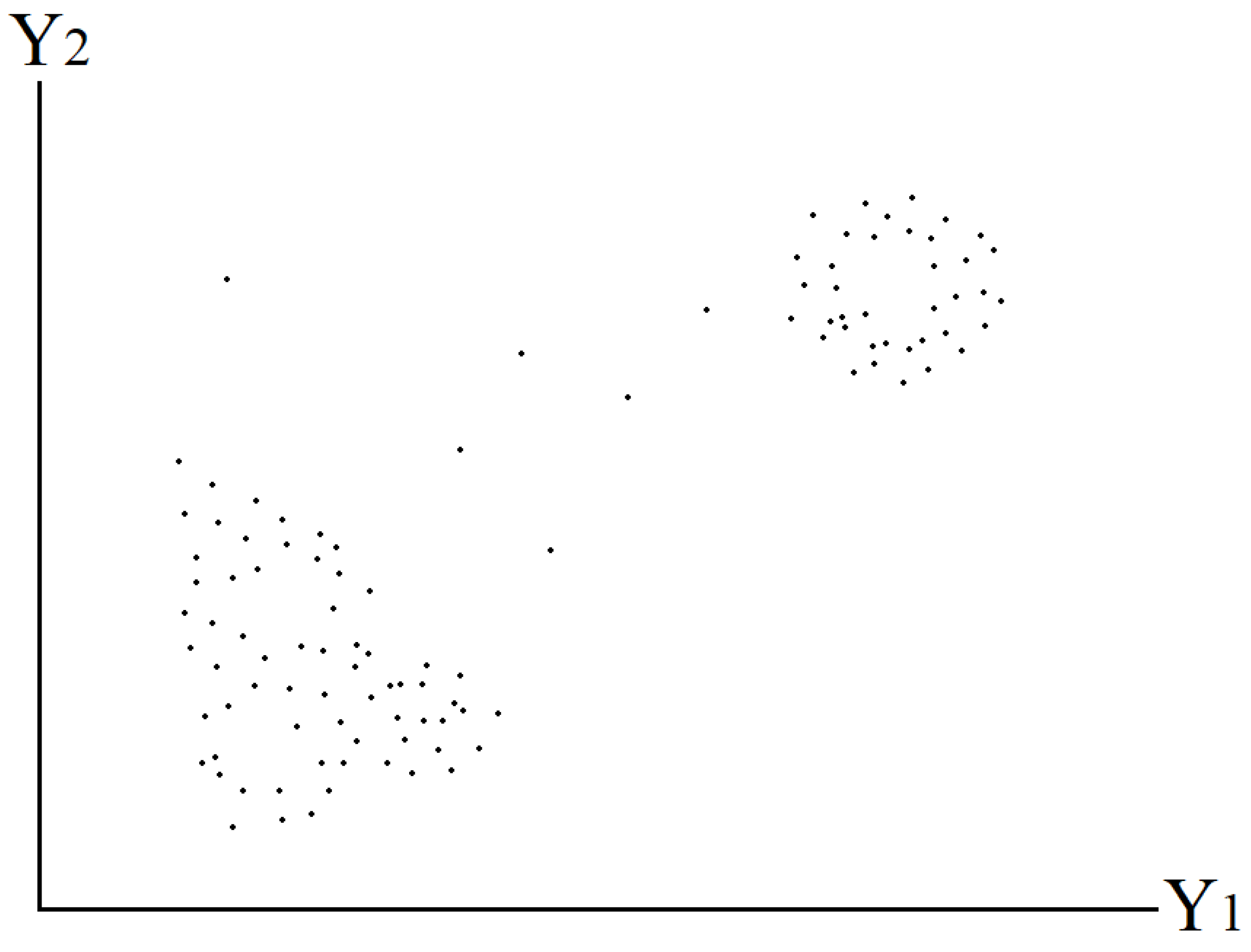
Using the following numerical illustration, we show how one can use the theory of TR in practice. Suppose that we have two risks, denoted by $Y_1,Y_2\in \mathbb{R}$, with historical data $Data={\left\{\left({\widehat{y}}_{1i},{\widehat{y}}_{2i}\right)\right\}}_{i=1}^m$. Then, we can plot the collected historical data $Data$.

In Figure 1, we observe that, in such example, the data are mainly divided by two different clusters. To build a regression model, one may use linear or nonlinear regression models, but such models must take into account that the data are of two separated clusters, and thus, for example, a linear regression would not provide a good predictive model for the data. Furthermore, the topological structure of the two clusters should also be considered. The following figure shows the topological structures of the data set, showing a two topological structure.

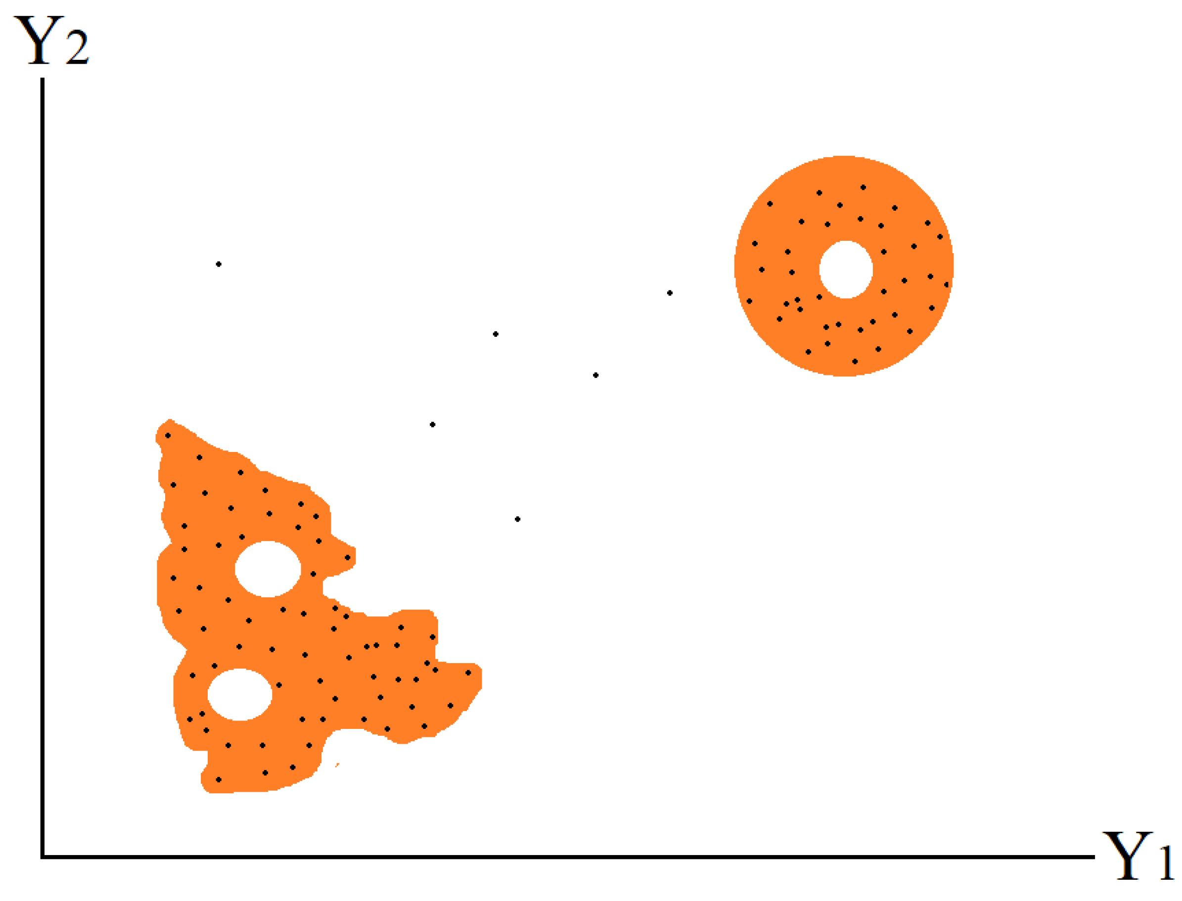
Figure 2 shows two topological risks for the two clusters of the dataset. As can be seen, the below-left cluster is illustrated by a genus-2 topological surface and the above-right cluster is illustrated by a torus. These two topologies construct the set of predicted outcomes for the pair $\left(Y_1,Y_2\right)$. Thus, any regression model for the risks should take into account such inner structure of the clusters. Furthermore, any risk measure $\varrho \left(\left(Y_1,Y_2\right)\right)\in {\mathbb{R}}^2$ would be on the domain of the topological risks. For example, the following topological-based risk measure can be obtained by taking the conditional expectation of the risks $Y_1,Y_2,$ as follows:

$$\varrho \left(\left(Y_1,Y_2\right)\right)=E\left({\left(Y_1,Y_2\right)}^T|\left(Y_1,Y_2\right)\in \mathrm{Top}\left(Y\right)\right),$$

where Top$\left(Y\right)$ is the topological structure of the data; in our example, it is the orange area in Figure 2 with a torus and genus-2 structures.

4. Discussion

In this paper, we have investigated the use of topology for studying risks. We have shown how topological risks can be divided into two general classes of risks, namely, diversifiable and non-diversifiable risks, and we have presented a rigorous foundation for the topological risk theory. Although it is an intuitive result, using the theory provided here, we have shown that combining a pair of disjoint diversifiable topological risks into a single topological risk is also diversifiable. Furthermore, we have investigated the Euler characteristic for a portfolio of topological risks with applications in the theory of risks and provided some of its fundamental properties. We then presented some special dispersion measures that are based on the concept of a distance metric of the topological sets. The presented theory of topological risks provides a new formalism in risk measurement that has the potential for a future research.