Article

Calendar Spread Exchange Options Pricing with Gaussian Random Fields

Institute of Statistics, Biostatistics and Actuarial Sciences, University Catholique de Louvain, Voie du Roman Pays 20, 1348 Louvain-la-Neuve, Belgium
Risks 2018, 6(3), 77; https://doi.org/10.3390/risks6030077
Submission received: 6 July 2018 / Revised: 31 July 2018 / Accepted: 2 August 2018 / Published: 8 August 2018

Abstract

:
Most of the models leading to an analytical expression for option prices are based on the assumption that underlying asset returns evolve according to a Brownian motion with drift. For some asset classes like commodities, a Brownian model does not fit empirical covariance and autocorrelation structures. This failure to replicate the covariance introduces a bias in the valuation of calendar spread exchange options. As the payoff of these options depends on two asset values at different times, particular care must be taken for the modeling of covariance and autocorrelation. This article proposes a simple alternative model for asset prices with sub-exponential, exponential and hyper-exponential autocovariance structures. In the proposed approach, price processes are seen as conditional Gaussian fields indexed by the time. In general, this process is not a semi-martingale, and therefore, we cannot rely on stochastic differential calculus to evaluate options. However, option prices are still calculable by the technique of the change of numeraire. A numerical illustration confirms the important influence of the covariance structure in the valuation of calendar spread exchange options for Brent against WTI crude oil and for gold against silver.

1. Introduction

Gaussian fields have been used for several decades in the analysis of spatial statistics. One of the key features in spatial statistics is the autocorrelation of data. The observations at locations in close spatial proximity often tend to be more similar than observations at locations far apart. We refer the interested reader to the books of Cressie (1993), Adler (1981) or Matern (1986) for a detailed presentation of spatial statistics and the theory of Gaussian fields. An introduction to Gaussian processes on general parameter spaces may be found in Adler and Taylor (2009).
We also find applications of Gaussian fields in the financial literature, e.g., Goldstein (2000) generalized the work of Kennedy (1994) and proposed a model for interest rates based on a two-dimensional random field. In this model, increments along time are independent, but the correlation structure between bond yields of different maturities can be arbitrarily chosen. The work in Kimmel (2004) introduced a state-dependent volatility in this model. Albeverio et al. (2004) extended previous models for yield curves with Lévy fields. The work in Ozkan and Schmidt (2009) used similar fields to model the yield curve in the presence of credit risk.
Gaussian fields are also used for actuarial modeling. The work in Biffis and Millossovich (2006) modeled the intensity of mortality as a random field, in order to capture cross-generation (risk class) effects induced by the on-going management of portfolios of policies. Based on this framework, Biagini et al. (2017) studied the pricing and hedging of life insurance liabilities. The work in Wu (2016) developed Gaussian process regression methods for mortality forecasting.
The pricing of exotic options with a payoff involving asset prices at different times requires a model able to replicate the covariance of underlying securities. Assuming that asset returns are ruled by a Brownian motion with drift is convenient for mathematical developments. However, this model does not replicate the time dependence observed for some asset classes as underlined by Willinger et al. (1999). On the other hand, option prices usually do not admit any closed form expressions for models with stronger econometric foundations. These points motivate this research that has a two-fold objective. Firstly, we propose a Gaussian model that is analytically tractable, with three possible covariance structure for asset prices. Secondly, we aim to emphasize the importance of the covariance in the valuation of exotic derivatives. For this purpose, we derive closed form expressions for calendar exchange spread and Asian calendar exchange spread options. Next, we evaluate in numerical applications the bias induced by a misspecification of the covariance structure.
In our approach, asset prices are seen as Gaussian fields indexed by time. These fields are conditional in the sense that their initial value is known. We work with homogeneous fields: the covariance only depends on the length of the time interval between considered prices. We study three covariance structures with sub-exponential, exponential and hyper-exponential autocorrelation functions. After a presentation of model features, we propose a method to simulate conditional Gaussian fields based on the spectral decomposition of the covariance function. Within this approach, a simulated sample path is known continuously at all times. This characteristic is particularly useful for pricing path-dependent options.
In order to emphasize the role played by the correlation on option prices, we evaluate two exotic derivatives with a payoff depending on asset prices at different times. The first one is the calendar spread exchange option. This option pays the positive difference between two asset prices observed at different times. The second derivative is an Asian calendar spread exchange option with geometric averages. This product pays the positive difference between the geometric average returns of two assets, calculated over different time intervals. Asian options with arithmetic averages are not studied as their price does not admit any closed form expression. In the numerical illustration, we calibrate our models to two pairs of assets (Brent-West Texas Intermediate (WTI) crude oil, silver-gold) and evaluate exchange options. Our results confirm that the misspecification of the autocorrelation function has a strong impact on the prices of calendar spread exchange options.

2. Conditional Gaussian Fields

We consider a probability space Ω , F , Q endowed with the filtration F t t 0 on which is defined a random field X t indexed by time. Before detailing the features of asset prices, we recall in this section the main properties of Gaussian random fields. A real valued random field is a family of random variables X t indexed by t R + with a collection of distribution functions of the form F t 1 , , t n :
F t 1 , , t n ( b 1 , , b n ) = P X t 1 b 1 , , X t n b n ,
where b 1 , , b n R . In this article, we consider Gaussian random fields for which the distribution F t 1 , , t n ( . ) is a multivariate normal distribution with a zero mean, E X t = 0 . This distribution is fully characterized by its covariance matrix. The covariance between X t and X s is denoted by C ( t , s ) . This is a non-negative definite function on R + × R + . Given that the mean of the Gaussian field is null, the covariance function is equal to its cross expectation:
C t , s = C X t , X s = E X t X s .
If the covariance function is equal to C ( t , s ) = t s , the Gaussian field is a pure Brownian motion with independent increments. However, a Gaussian field does not have in general independent increments and is not a Markov process. On the other hand, a Gaussian field is not systematically a semi-martingale. If the Gaussian field is not a semi-martingale, we cannot rely on stochastic differential calculus for evaluating options. In counterpart, working with Gaussian fields allows us to reproduce with accuracy the autocovariance function of asset prices compared to processes with independent increments. We will see later that this feature is particularly important for pricing calendar options. In this article, we consider continuous and differentiable covariance functions, C ( t , s ) C , and focus on the homogeneous Gaussian random field. A random field is homogeneous or stationary if E X t 2 is finite for all t and:
  • E X t is constant and independent of t R + ,
  • C t , s solely depends on the difference | s t | .
When the Gaussian field is homogeneous, the covariance function may be rewritten as a function g : R R + ,
g ( h ) = C ( t , t + h ) , = C X t + h , X t .
The construction of the function g ( . ) is detailed in the next section. For homogeneous fields, increments in the t direction are correlated. For t , h R + , the time covariance is equal to:
C X t + u X t , X t = C X t + u , X t C X t , X t , = g u g ( 0 ) .
This is a clear difference from the Brownian motion, which has independent increments. Furthermore, the conditional expectation of X s with respect to the filtration F t depends on the whole sample path of the process and not exclusively on X t . In general, X t is then not a Markov process1.
In financial applications, X 0 is known at Time 0 and will determine the asset prices. Therefore, we must determine the conditional distribution of X t with respect to X 0 . Given that X t , X 0 is a bivariate Gaussian distribution:
X t X 0 d N 0 0 , g ( 0 ) g ( t ) g ( t ) g ( 0 ) ,
The random variable Z t X t | X 0 = x is Gaussian d N μ t | x , σ t | x 2 with a mean and variance given by:
μ t | x = 0 + g ( t ) g ( 0 ) x 0 , σ t | x 2 = g ( 0 ) g ( t ) 2 g ( 0 ) .
Using the properties of the multivariate normal distribution, we directly infer the covariance between Z t and Z s in the next proposition that is used in later developments.
Proposition 1.
The joint distribution of Z t = X t | X 0 = x and Z s = X s | X 0 = x for 0 t s is a bivariate normal random variable with a mean and covariance matrix given by:
Z s Z t d N g ( s ) g ( 0 ) x g ( t ) g ( 0 ) x , g ( 0 ) g ( s ) 2 g ( 0 ) g ( s t ) g ( s ) g ( t ) g ( 0 ) g ( s t ) g ( s ) g ( t ) g ( 0 ) g ( 0 ) g ( t ) 2 g ( 0 ) .
In the next section, we consider covariance functions of homogeneous fields that are decreasing functions of h such that lim h g ( h ) = 0 . From the previous proposition, we infer the asymptotic variance and covariance of Z t :
lim s V Z s | F 0 = g ( 0 )
and:
lim s C Z t , Z s | F 0 = 0 .
The variance being bounded by a constant, the process Z t reverts around its mean.
If X t is a Brownian field, the covariance between X t and X s for 0 t s is equal to C X t , X s = s t = t . Conditional to X 0 , Z t = X t | X 0 = x and Z s = X s | X 0 = x are distributed according to a bivariate normal distribution with a mean x , x and a covariance matrix s t t t . In this particular case, when t , the variance tends to infinity, and the covariance is equal to t:
lim s V Z s | F 0 = lim s C Z t , Z s | F 0 = t .
Therefore, homogeneous fields have a very different behavior from the Brownian motion. As their variance is asymptotically constant, homogeneous fields revert to their mean and are not adapted to model stock prices, which usually have a variance increasing with the time horizon. This property makes them more suitable for the modeling of interest rates or any assets with a mean reverting yield. The proposed approach is also appropriate for commodities; mainly because their value reverts to a long run equilibrium level with a constant asymptotic variance as illustrated in Bessembinder et al. (1995). Gibson and Schwartz (1990); Cortazar and Schwartz (1994); Schwartz (1997) or Hainaut (2017) modeled commodities with an Ornstein–Uhlenbeck (OU) process presenting the same features as those of Equation (1).

3. Market Model

The filtration F t t 0 is generated by d independent continuous and homogeneous random fields X t ( k ) for k = 1 to d. They have a null mean, and the covariance function of X t ( k ) is denoted by g k ( h ) C k ( t , t + h ) where g k : R R + and g k ( h ) = g k ( h ) . The processes X t ( k ) are homogeneous in time, but increments of the random field in the t direction are correlated: for t , h R + , we have that C X t + u ( k ) X t ( k ) , X t ( k ) = g k u g k ( 0 ) . Furthermore, g k ( 0 ) = 1 and X 0 ( k ) = 0 . The probability measure Q is here the probability measure under which the pricing of financial derivatives is done. As in the previous section, we denote by Z t ( k ) the expectation of X t ( k ) conditional to X 0 ( k ) = 0 :
Z t ( k ) X t ( k ) | X 0 ( k ) = 0 k = 1 , , d .
The risk-free rate is assumed constant and is denoted r. We assume that the financial market counts two securities, S t ( 1 ) and S t ( 2 ) , with a homogeneous covariance structure. The yields2 of these assets are denoted by y t ( 1 ) and y t ( 2 ) . The relation between yields and prices is S t ( j ) = S 0 ( j ) exp y t ( j ) for j = 1 , 2 . We denote the vector of conditional Gaussian fields by Z t = Z t ( 1 ) , , Z t ( d ) . In our model, the yields are linear functions of Gaussian fields:
y t ( 1 ) y t ( 2 ) = r + c 1 t α 1 ( t ) r + c 2 t α 2 ( t ) + σ 11 σ 12 σ 1 d σ 21 σ 22 σ 2 d Σ Z t ,
where α j ( t ) for j = 1 , 2 are functions from R + to R + equal to:
α j ( t ) 1 2 k = 1 d σ j k 2 1 g k ( t ) 2 .
Σ is a 2 × d real matrix3. c 1 and c 2 are adjustments of the drift for non-financial assets like commodities. Under the risk-neutral measure, commodities earn on average the risk-free rate plus the cost of carry and less the convenience yield. If S t ( 1 ) and S t ( 2 ) are financial assets, these factors are null: c 1 = c 2 = 0 . According to the usual financial theory, discounted financial security prices must be martingale processes under the pricing measure Q. More precisely if Σ j , . is the j t h line of Σ , discounted prices are such that E e r T S T ( j ) | F t = S 0 ( j ) E e α j ( T ) + Σ j , . Z T | F t for any times t T . Except in the case of the Brownian motion, a time Gaussian field depends in general on its sample path in a complex manner, and the process is not Markovian. Therefore, the expectation E e Σ j , . Z T | F t does not admit a closed form solution, and the drift α j ( T ) that ensures that discounted prices are always martingale is unknown4. However, at time t = 0 , the martingale condition E e r T S T ( j ) | F 0 = S 0 ( j ) is fulfilled if α j ( t ) are defined by Equation (3). If S t ( 1 ) and S t ( 2 ) are non-financial assets, their future price is equal to E S T ( j ) | F 0 = S 0 ( j ) e ( r + c j ) T for j = 1 , 2 , and this relation holds only if α j ( t ) are defined by Equation (3).
If we remember Proposition 1 and given that g k ( 0 ) = 1 , the autocovariance of y t ( j ) is:
C y t ( j ) , y s ( j ) | F 0 = k = 1 d σ j k 2 g k ( s t ) g k ( s ) g k ( t ) f o r j = 1 , 2 ,
whereas the covariance of y t ( 1 ) and y s ( 2 ) is equal to:
C y t ( 1 ) , y s ( 2 ) | F 0 = E y t ( 1 ) y s ( 2 ) | F 0 E y t ( 1 ) | F 0 E y s ( 2 ) | F 0 , = k = 1 d σ 1 k σ 2 k g k ( s t ) g k ( s ) g k ( t ) .
We remark that this is an important difference with existing models using Gaussian fields, e.g., Goldstein (2000) or Kennedy (1994) developed a model for interest rates in which time increments are independent. In this particular case, the Gaussian field is a semi-martingale, and we can use the Itô’s calculus to deduce the main properties of asset dynamics.

4. Choice of Autocovariance Functions

In this article, we consider three types of autocovariance functions that are built with Bochner’s theorem. A function g ( h ) is eligible to be an autocovariance function if it is positive definite. The work in Bochner (1993) showed that positive definite functions may be defined by their spectral measure.
Theorem 1.
(Bochner) A continuous function g ( h ) from R + to the complex plane C is positive definite if and only if it may be represented as the Fourier transform of a measure ν ( . ) on R :
g ( h ) = R e i h u ν ( d u ) ,
where ν ( . ) is a bounded, real valued function such that A ν ( d u ) 0 for all A R .
The function ν ( . ) is called the spectral distribution function for g. An alternative representation is:
g ( h ) = R cos h u + i sin h u ν ( d u ) .
Then, if Z t is R -valued, g ( h ) is also R -valued, and the imaginary part in this last equation is null: R sin h u ν ( d u ) = 0 . This implies that the spectral distribution is symmetric around the origin. If ν ( . ) is continuous, we then have ν ( d u ) = ν ( d u ) and:
g ( h ) = R cos h u ν ( d u ) , = 2 0 cos | h | u ν ( d u ) .
In this work, we consider three spectral distributions ν ( . ) : a double exponential, an inverse quadratic and a double quadratic exponential measure. The next paragraphs detail each one.
(1) The first measure considered is the double exponential measure. Let λ R + be constant. A symmetric exponential measure is defined by the following relation:
ν ( d u ) = 1 2 λ e λ u 1 { u 0 } + λ e λ u 1 { u 0 } d u .
If we use this function as the spectral distribution of the covariance, we obtain the following function g ( h ) :
g ( h ) = 1 2 R + λ e i h u e λ u d u + R λ e i h u e λ u d u = λ 2 λ 2 + h 2 ,
which is a sub-exponential function (in the sense that it decays at a lower pace than an exponential function). In order to define autocovariance functions of Gaussian fields Z t ( k ) involved in the dynamics of the financial market, we consider d spectral density functions (4) parameterized by a vector λ = { λ 1 , , λ d } R d + . The corresponding autocovariance functions are in this case denoted g k s u b ( . ) and defined by:
g k s u b ( h ) λ k 2 λ k 2 + h 2 k = 0 , 1 , , d .
(2) The second type of spectral measure that we study is the inverse quadratic one:
ν ( d u ) = 1 π λ λ 2 + u 2 d u ,
where λ R + . By construction, this measure is symmetric, and the function g ( h ) is an exponential decreasing function:
g ( h ) = 2 λ π R + cos | h | u λ 2 + u 2 d u = e λ | h | .
It may be shown that this autocovariance function is closely related to the one of an Ornstein–Uhlenbeck process. Details are provided in Appendix A. In later developments, we consider d exponential autocovariance functions for Z t ( k ) parameterized by λ = { λ 1 , , λ d } R d , + and denoted by:
g k e x p ( h ) e λ k | h | k = 0 , 1 , , d .
(3) The last category of covariance functions is generated with what we call an exponential quadratic spectral measure:
ν ( d u ) = λ π e λ u 2 d u .
Given that R + e λ u 2 cos h u d u = 1 2 π λ e h 2 4 λ , the autocovariance function is in this case equal to:
g ( h ) = 2 λ π R + e λ u 2 cos | h | u d u = e h 2 4 λ .
We abusively call this covariance function the exponential quadratic covariance. This function decays at a faster pace than an exponential one and is in this sense hyper-exponential decreasing. In the following sections, we consider d exponential quadratic covariance functions for Z t ( k ) parameterized by λ = { λ 1 , , λ d } R d , + and denoted as:
g k q u a ( h ) = e h 2 4 λ k k = 0 , 1 , , d .
We will price calendar spread exchange options using these three autocovariance functions g k s u b ( h ) , g k e x p ( h ) and g k q u a ( h ) . As autocovariance functions g k s u b ( h ) and g k q u a ( h ) decrease respectively at a lower and at a faster pace than g k e x p ( h ) , our approach covers a wide spectrum of autocorrelation structures.
Options are priced under the risk-neutral measure, and autocovariance functions should therefore duplicate option market prices. However, if the option market is not liquid enough, an alternative solution to calibrate g k ( . ) consists of assuming that covariances under the pricing and real measures are similar (eventually adjusted by a risk premium). Under this assumption, the functions g k ( . ) { g k s u b ( . ) , g k e x p ( . ) , g k q u a ( . ) } can easily be calibrated with the method of moments matching. In this case, we minimize the quadratic spread between marginal and empirical covariances denoted by C ^ X . , X . + Δ h :
{ Σ , λ } = arg min h = 0 H k = 1 d σ 1 k 2 g k ( h Δ ) C ^ y . ( 1 ) , y . + h Δ ( 1 ) 2 + h = 0 H k = 1 d σ 2 k 2 g k ( h Δ ) C ^ y . ( 2 ) , y . + h Δ ( 2 ) 2 + h = 0 H k = 1 d σ 1 k σ 2 k g k ( h Δ ) C ^ y . ( 1 ) , y . + h Δ ( 2 ) 2 ,
where Δ is the time interval between two successive observations. This approach is applied in numerical illustrations in order to determine which covariance function is the most suitable for some commodity prices (silver, gold, Brent and WTI crude oil).

5. Simulation of a Conditional Field by Spectral Decomposition

In this section, we propose a method to simulate sample paths of asset prices. As increments of Gaussian fields involved in the dynamics of S t ( 1 ) and S t ( 2 ) are not independent, the simulation of these processes requires particular care. A natural approach consists of simulating the asset dynamics with a multivariate normal distribution conditioned by X 0 = 0 , on a discrete time grid. However, there exists an elegant alternative based on a discretization in the space of frequencies. With this approach, the sample path of S t ( 1 ) and S t ( 2 ) is known at all times t and not only at discrete times. This feature is particularly interesting for the pricing of path-dependent options. Let us first recall that the covariance function of a homogeneous Gaussian field is defined by a measure ν ( . ) . In the developments of Section 4, we have considered a (probability) measure5 ν ( . ) of R . For any Borel subset A R , we note ν ( A ) = A ν ( d u ) . We define a complex noise W based on the measure ν , or ν -noise, as a random process defined on Borel subsets of R , such that for all A , B B with ν ( A ) and ν ( B ) finite, we have:
E W ( A ) = 0 , E W ( A ) W ( A ) ¯ = ν ( A ) , A B = W ( A B ) = W ( A ) + W ( B ) a . s . , A B = , E W ( A ) W ( B ) ¯ = 0 .
When the measure ν ( . ) is the Lebesgue measure and W ( A ) d N ( 0 , ν ( A ) ) , W is a white noise and more precisely a Brownian motion. Having defined complex ν -noises, we build the integral with respect to W, of a function φ ( t ) : R C such that φ ( x ) 2 ν ( d x ) < . By analogy with the Riemann integral, the integral of φ ( t ) over an interval R with respect to W is defined as the limit of a sum over a partition Π n = [ t k , t k + 1 ] k = 0 , , n 1 of [ 0 , T n ] :
W ( φ ) R φ ( u ) W ( d u ) lim T n , n k = 0 n 1 W ( [ t k , t k + 1 ] ) φ t k .
By construction, R φ ( u ) W ( d u ) is a random variable that has zero mean and variance given by R φ t 2 ν ( d t ) . On the other hand, given that E W ( A ) W ( B ) ¯ = 0 if A B = , we have that:
E W ( φ ) W ( ψ ) ¯ = R φ ( t ) ψ ( t ) ¯ ν ( d t ) .
This construction allows us to state a useful representation theorem:
Theorem 2.
(Spectral representation theorem) Let ν be a finite measure on R and W complex ν-noises. Then, the complex valued random field:
X t = R e i ( t u ) W ( d u ) ,
has a covariance function:
C ( t , s ) = g ( s t ) = R e i ( ( s t ) u ) ν ( d u ) .
If W is Gaussian, then so is X t . Furthermore, to every mean-square centered (Gaussian) stationary random field on R , with covariance function C and spectral measure, there corresponds a complex (Gaussian) ν -noise W on R such that Equation (10) holds in the mean square for each t R N . In both cases, W is called the spectral process corresponding to X t .
In one direction, the proof of this theorem is immediate. It is a consequence of the construction of the stochastic integral W ( φ ) that X t defined by Equation (10) has covariance function (11). The other direction is less direct, and we refer to the book of Adler and Taylor (2007) for a proof (Theorem 2).
In this article, we consider a real Gaussian field X t with a symmetric spectral measure. Then, its covariance function can be rewritten as follows:
C ( t , s ) = R cos ( s t ) u ν ( d u ) = R + cos ( s t ) u μ ( d u )
where we have defined a positive measure μ ( A ) = 2 ν ( A ) for all A R + . In Section 4, we have introduced three symmetric measures leading to three types of covariance. The measure μ ( . ) for each of these cases is given by:
μ s u b ( d u ) = λ e λ u d u , μ e x p ( d u ) = 2 π λ λ 2 + u 2 d u , μ q u a ( d u ) = 2 λ π e λ u 2 d u .
The next proposition shows that we can reformulate the Gaussian field as integrals with respect to μ -noises:
Proposition 2.
A Gaussian field X t with a covariance function (12) can be rewritten as the sum of two integrals with respect to independent real (Gaussian) valued μ -noises W 1 and W 2 such that:
X t = R + cos u t W 1 ( d u ) + R + sin u t W 2 ( d u )
The proof is reported in Appendix B. In practice, we use Equation (13) to approximate the sample path of X t ( k ) over a partition { u 0 , u 1 , , u n } of R + (with u 0 = 0 ) as follows:
X t ( k ) j = 0 n cos t u j W 1 ( k ) ( [ u j , u j + 1 ) ) + sin t u j W 2 ( k ) ( [ u j , u j + 1 ) ) .
where W 1 ( k ) ( . ) and W 2 ( k ) ( . ) are normal random variables:
W 1 ( k ) ( [ u j , u j + 1 ) ) d N 0 , μ ( k ) [ u j , u j + 1 ) , W 2 ( k ) ( [ u j , u j + 1 ) ) d N 0 , μ ( k ) [ u j , u j + 1 ) .
If the measure is double-exponential (and the function g is sub-exponential), then the measure of a time interval is equal to:
μ ( k ) [ u j , u j + 1 ) = u j u j + 1 λ k e λ k u d u = e λ k u j e λ k u j + 1 .
If the measure is inverse quadratic (and the function g is exponential), then the measure of a time interval is equal to:
μ ( k ) [ u j , u j + 1 ) = 2 π u j u j + 1 λ λ 2 + u 2 d u = 2 π arctan u j + 1 λ arctan u j λ .
If the function g is exponential quadratic, then:
μ ( k ) [ u j , u j + 1 ) = u j u j + 1 2 λ π e λ u 2 d u = erf λ u j + 1 erf λ u j .
The number of intervals n and u n is chosen such that the variance e λ k u j e λ k u j + 1 , of W 1 ( k ) and W 2 ( k ) , is close to zero. Equation (14) allows us to simulate a Gaussian field X t that is not conditioned by its initial value X 0 . In order to simulate Z t ( k ) X t ( k ) | X 0 ( k ) = 0 for k = 1 , , d , we need to take into account the constraint X 0 ( k ) = 0 . With regards to Equation (14), X 0 ( k ) = 0 if and only if the following random variable is null:
H j = 0 n W 1 ( k ) ( [ u j , u j + 1 ) ) = 0 .
By construction, the random vector W ¯ 1 ( k ) = W 1 ( k ) ( [ u j , u j + 1 ) ) j = 0 , , n is a multivariate normal N 0 n + 1 ; Σ k , where 0 n + 1 is a null vector of dimension n + 1 and Σ k is a ( n + 1 ) × ( n + 1 ) matrix of covariance:
Σ k diag μ ( k ) [ u 0 , u 1 ) , , μ ( k ) [ u j , u j + 1 ) , , μ ( k ) [ u n 1 , u n ) .
Therefore, the covariance between W 1 ( k ) ( [ u j , u j + 1 ) ) and H is equal to μ ( k ) [ u j , u j + 1 ) . The variance of H is equal to 1 n + 1 Σ k 1 n + 1 where 1 n + 1 is an n + 1 vector of ones. The vector W ¯ 1 ( k ) , H is a multivariate normal distribution with the following mean and covariance:
W ¯ 1 ( k ) H d N 0 n + 2 ; Σ k Σ k 1 n + 1 1 n + 1 Σ k 1 n + 1 Σ k 1 n + 1 .
Using the properties of the conditional Gaussian multivariate distribution, we have that B ¯ ( k ) W ¯ 1 ( k ) | H = 0 is also a multivariate normal N 0 n + 1 ; Σ W ¯ 1 ( k ) | H = 0 with a covariance matrix:
Σ W ¯ 1 ( k ) | H = 0 Σ k Σ k 1 n + 1 1 n + 1 Σ k 1 n + 1 Σ k 1 n + 1 ,
and where 1 n + 1 Σ k Σ k 1 n + 1 is a n + 1 × n + 1 matrix:
Σ k 1 n + 1 1 n + 1 Σ k = μ ( k ) [ u 0 , u 1 ) 2 μ ( k ) [ u 0 , u 1 ) μ ( k ) [ u n 1 , u n ) μ ( k ) [ u 0 , u 1 ) μ ( k ) [ u n 1 , u n ) μ ( k ) [ u n 1 , u n ) 2 .
In numerical illustrations, the sample path of Z t ( k ) over a partition { u 0 , u 1 , , u n } of R + (with u 0 = 0 ) is then simulated with the following relation:
Z t ( k ) j = 0 n cos t u j B ( k ) ( [ u j , u j + 1 ) ) + sin t u j W 2 ( k ) ( [ u j , u j + 1 ) ) .
where B ¯ ( k ) d N 0 n + 1 ; Σ W ¯ 1 ( k ) | H = 0 and W 2 ( k ) ( . ) are normal random variables:
W 2 ( k ) ( [ u j , u j + 1 ) ) d N 0 , μ ( k ) [ u j , u j + 1 ) .
This technique allows for simulating the sample path of Z t , which are known for all times t R + . This method is particularly helpful for the pricing of path-dependent options.

6. Calendar Spread Exchange Options Pricing

One objective of this article is to emphasize the importance of the autocorrelation in the valuation of exotic derivatives. For this purpose, we derive closed form expressions for calendar spread exchange options and for Asian options of the same type in the next section. Next, we will assess numerically the bias induced by a misspecified covariance structure. A calendar spread exchange European option is a financial derivative delivering a payoff equal to the positive difference between β 1 S T ( 1 ) and β 2 S t ( 2 ) , at expiry T. The price of this option is equal to the expected discounted payoff under the risk-neutral measure:
E e r T ( β 1 S T ( 1 ) β 2 S t ( 2 ) ) + | F 0 .
Gaussian fields Z t ( k ) have sub-exponential, exponential or exponential quadratic autocovariance functions: g k { g k s u b ( . ) , g k e x p ( . ) , g k q u a ( . ) } for k = 1 , , d . In order to obtain a closed form expression for the option price, we introduce a new probability measure, denoted by Q S 2 . This measure uses S t ( 2 ) as numeraire. The change of measure from Q to Q S 2 is defined by the following random variable:
d Q S 2 d Q = S t ( 2 ) S 0 ( 2 ) 1 e ( r + c 2 ) t , = exp α 2 ( t ) + Σ 2 , . Z t
where α 2 ( t ) = 1 2 k = 1 d σ 2 k 2 1 g k ( t ) 2 and Σ 2 , . is the second line of the matrix Σ . This approach was used by Margrabe (1978) so as to evaluate the exchange option in a Brownian setting. By definition, d Q S 2 d Q is a strictly positive, F t -measurable random variable such that E d Q S 2 d Q | F 0 = 1 . Conditional to F 0 , it defines then an equivalent measure Q S 2 to Q. For any F T -adapted random variable N T , we have the following relation:
E Q S 2 N T S t ( 2 ) | F 0 = E d Q S 2 d Q N T S t ( 2 ) | F 0 E d Q S 2 d Q | F 0 , = S 0 ( 2 ) e ( r + c 2 ) t 1 E N T | F 0 .
We immediately infer from this last expression that the expectation of N T under Q is also equal to:
E N T | F 0 = S 0 ( 2 ) e ( r + c 2 ) t E Q S 2 N T S t ( 2 ) | F 0 .
This result allows us to rewrite the calendar spread exchange option as follows:
e r T E ( β 1 S T ( 1 ) β 2 S t ( 2 ) ) + | F 0 = β 2 S 0 ( 2 ) e r ( T t ) + c 2 t E Q S 2 β 1 β 2 S T ( 1 ) S t ( 2 ) 1 + | F 0 .
The next step consists of determining the statistical distribution of S T ( 1 ) S t ( 2 ) under the measure Q S 2 . By construction, the ratio of asset prices is given by:
S T ( 1 ) S t ( 2 ) = S 0 ( 1 ) S 0 ( 2 ) exp r T t + c 1 T c 2 t α 1 ( T ) α 2 ( t ) + Σ 1 , . Z T Σ 2 , . Z t ,
where Σ 1 , . and Σ 2 , . point out the first and second line of the matrix Σ . Let us denote the logarithm of this ratio by:
R t , T = ln S T ( 1 ) S 0 ( 2 ) S t ( 2 ) S 0 ( 1 ) = r T t + c 1 T c 2 t α 1 ( T ) α 2 ( t ) + Σ 1 , . Z T Σ 2 , . Z t .
The statistical distribution of R t , T under the measure Q S 2 is Gaussian, as detailed in the next proposition proven in Appendix B:
Proposition 3.
R t , T under the measure Q S 2 is a normal random variable with a mean μ R ( t , T ) and a variance σ R ( t , T ) 2 equal to:
μ R ( t , T ) = r T t + c 1 T c 2 t α 1 ( T ) α 2 ( t ) + k = 1 d σ 1 k σ 2 k g k ( T t ) g k ( T ) g k ( t ) , σ R 2 ( t , T ) = 2 α 1 ( T ) + α 2 ( t ) k = 1 d σ 1 k σ 2 k g k ( T t ) g k ( T ) g k ( t ) .
The exchange option price as reformulated in Equation (17) is a call option on a lognormal underlying asset. As stated in the next proposition, the option price admits then a closed form expression similar to the Black and Scholes equation, and this result holds whichever the covariance function g k { g k s u b ( . ) , g k e x p ( . ) , g k q u a ( . ) } .
Proposition 4.
Let Φ x be the cumulative distribution function of a standard normal random variable. The price of a calendar spread exchange option price is given by the following expression:
e r T E ( β 1 S T ( 1 ) β 2 S t ( 2 ) ) + | F 0 = β 1 S 0 ( 1 ) e c 1 T Φ d 1 ( t , T ) β 2 S 0 ( 2 ) e r ( T t ) + c 2 t Φ d 2 ( t , T ) ,
where d 1 ( t , T ) and d 2 ( t , T ) are defined as follows:
d 2 ( t , T ) = ln β 2 β 1 S 0 ( 2 ) S 0 ( 1 ) μ R ( t , T ) σ R ( t , T ) ,
and:
d 1 ( t , T ) = d 2 ( t , T ) σ R ( t , T ) .
In Section 8, we evaluate calendar spread exchange options for Brent against WTI crude oil and for silver against gold.

7. Asian Calendar Spread Exchange Options, with the Geometric Average

Our approach presents the same level of tractability as a Brownian motion. To illustrate this point and to emphasize the role of the covariance structure on Asian options, we price another type of exotic derivative that depends on the whole sample path of asset prices. We focus on Asian calendar spread options with a payoff related to geometric average returns of assets S t ( 1 ) and S t ( 2 ) . Let us denote by G T ( 1 ) and G t ( 2 ) the geometric average returns of S s ( 1 ) s = 0 : T and S s ( 2 ) s = 0 : t with t T and defined as:
G T ( 1 ) e 1 T 0 T ln S s ( 1 ) S 0 1 d s , G t ( 2 ) e 1 t 0 t ln S s ( 2 ) S 0 ( 2 ) d s .
An Asian calendar spread exchange option pays the positive difference between β 1 G T ( 1 ) and β 2 G t ( 2 ) , at expiry T. The price of this option is the expected discounted payoff under the risk-neutral measure:
E e r T ( β 1 G T ( 1 ) β 2 G t ( 2 ) ) + | F 0 .
By definition, the log-return of assets is equal to:
ln S s ( j ) S 0 ( j ) = ( r + c j ) s α j ( s ) + Σ j , . Z s j = 1 , 2 .
Therefore, the integral of this log-return over the interval [ 0 , t ] , which is equal to ln G t ( j ) , is:
ln G t ( j ) = 1 t 0 t ln S s ( j ) S 0 ( j ) d s = 1 2 r + c j t 1 t 0 t α j ( s ) d s + 1 t Σ j , . 0 t Z s d s j = 1 , 2 .
Before any further developments, we present the properties of the integral of Z s ( k ) . This integral over [ 0 , T ] is defined as the limit of a sum over a partition Π n = [ t j , t j + 1 ] j = 0 , , n 1 of [ 0 , T ] :
0 T Z u ( k ) d u lim n j = 0 n 1 Z t j ( k ) t j + 1 t j .
Given that Z t j ( k ) is a Gaussian random variable, this integral is distributed as a normal random variable of a null mean under the condition that its variance exists. The variance of 0 T Z u ( k ) d u is obtained by considering the limit of the product of integrals over the partition Π n :
0 T Z u ( k ) d u 0 T Z u ( k ) d u = lim n i = 0 n 1 j = 0 n 1 Z t i ( k ) Z t j ( k ) t i + 1 t i t j + 1 t j .
As E Z t ( k ) | F 0 = 0 and Z t ( k ) for k = 1 , , d are independent processes, the expectation of this product with respect to F 0 is equal to the variance of 0 T Z u ( k ) d u :
V 0 T Z u ( k ) d u 0 T Z u ( k ) d u | F 0 = lim n i = 0 n 1 j = 0 n 1 C Z t i ( k ) Z t j ( k ) | F 0 t i + 1 t i t j + 1 t j . = 0 T 0 T g k ( u v ) g k ( u ) g k ( v ) d u d v .
This last double integral is bounded by T 2 g ( 0 ) for the three covariance functions that are considered in this article, and the integral 0 T Z u ( k ) d u is a normal random variable. The next propositions proven in Appendix B details the integrals involved in the expression (22) of the variance of 0 T Z u ( k ) d u for the three autocovariance functions { g k s u b ( . ) , g k e x p ( . ) , g k q u a ( . ) } .
Proposition 5.
Let ω C . If g k ( h ) = g k s u b ( h ) , then the double integral 0 t 0 T g k ( u v ) d v d u is equal to:
0 t 0 T g k ( u v ) d v d u = t λ k tan 1 t λ k 1 2 λ k 2 ln 1 + t 2 λ k 2 + λ k T t tan 1 t T λ k + 1 2 λ k 2 ln 1 + t T λ k 2 λ k T tan 1 T λ k + 1 2 λ k 2 ln 1 + T λ k 2 ,
whereas the double integral 0 t 0 T g k ( u ) g k ( v ) d v d u is given by:
0 t 0 T g k ( u ) g k ( v ) d v d u = λ k 2 tan 1 t λ k tan 1 T λ k .
From the definition (21) of ln G t ( j ) , the variance of G t ( j ) is equal to 1 t 2 V Σ j , . 0 t Z s d s | F 0 .
σ ln G j ( t ) 2 1 t 2 V Σ j , . 0 t Z s d s | F 0 .
From Equation (22) and Proposition 5, we immediately infer the next corollary:
Proposition 6.
If covariance functions are sub-exponential, g k ( h ) = g k s u b ( h ) , the variance of ln G t ( j ) , denoted by σ ln G j ( t ) 2 , is equal to:
σ ln G j ( t ) 2 1 t 2 k = 1 d σ j k 2 2 t λ k tan 1 t λ k λ k 2 ln 1 + t 2 λ k 2 λ k tan 1 t λ k 2 ,
for j = 1 , 2 .
The drift of ln G t ( j ) depends on the integral of α j ( . ) . The next proposition proven in Appendix B provides the analytical integral of this function when the covariance is sub-exponential.
Proposition 7.
If covariance functions are sub-exponential, g k ( h ) = g k s u b ( h ) , then the integral of function α j ( . ) is given by:
1 t 0 t α j ( s ) d s = 1 2 k = 1 d σ j k 2 1 λ k 2 t tan 1 t λ k λ k 2 2 t 2 + λ k 2 ,
for j = 1 , 2 .
If the covariance function is exponential, then the double integrals needed to evaluate the variance of 0 t Z s d s in Equation (22) are given by the following proposition detailed in Appendix B.
Proposition 8.
Let ω C . If g k ( h ) = g k e x p ( h ) , then the double integral 0 t 0 T g k ( u v ) d v d u is equal to:
0 t 0 T g k ( u v ) d v d u = 2 t λ k 1 λ k 2 1 e λ k t + 1 λ k 2 e λ k T e λ k ( t T ) ;
whereas the double integral 0 t 0 T g k ( u ) g k ( v ) d v d u is given by:
0 t 0 T g k ( u ) g k ( v ) d v d u = 1 λ k 2 1 e λ k t 1 e λ k T .
A direct corollary of this proposition is that the variances of ln G t ( j ) for j = 1 , 2 admit a closed form expression:
Proposition 9.
If autocovariance functions are exponential g k ( h ) = g e x p ( h ) , the variance of ln G t ( j ) , denoted by σ ln G j ( t ) 2 , is equal to:
σ ln G j ( t ) 2 1 t 2 k = 1 d σ j k 2 2 t λ k 1 λ k 2 1 e λ k t 1 λ k 2 1 e λ k t 2 ,
for j = 1 , 2 .
The drift of ln G t ( j ) depends on the integral of α j ( . ) which is provided in the next proposition, proven in Appendix B.
Proposition 10.
If autocovariance functions are exponential, g k ( h ) = e λ k h , then:
1 t 0 t α j ( s ) d s = 1 2 1 t k = 1 d σ j k 2 t 1 2 λ k 1 e 2 λ k t ,
for j = 1 , 2 .
When covariance functions are exponential quadratic, the integrals involved in the variance of ln G t ( j ) are given in the following proposition:
Proposition 11.
Let ω C and e r f ( x ) = 2 π 0 x e t 2 d t be the error function. If g k ( h ) = g k q u a d ( h ) , then:
0 t 0 T g k ( u v ) d v d u = π λ k t e r f t 2 λ k 2 λ k 1 e t 2 4 λ k π λ k ( T t ) e r f T t 2 λ k + π λ k T e r f T 2 λ k 2 λ k e t T 2 4 λ k e T 2 4 λ k ,
and:
0 t 0 T g k ( u ) g k ( v ) d v d u = π λ k e r f t 2 λ k e r f T 2 λ k .
When the covariance functions are quadratic exponential, the variance of ln G t ( j ) for j = 1 , 2 is given by the next proposition:
Proposition 12.
If the autocovariance functions g k ( h ) are defined by Equation (8), then the variance of ln G t ( j ) , denoted by σ ln G j ( t ) 2 is equal to:
σ ln G j ( t ) 2 1 t 2 k = 1 d σ j k 2 2 λ k π t e r f t 2 λ k 4 λ k 1 e t 2 4 λ k λ k π e r f t 2 λ k 2 ,
for j = 1 , 2 .
The drift of ln G t ( j ) depends on the integral of α j ( . ) . The next proposition proven in Appendix B provides the analytical integral of this function when the covariance is quadratic exponential.
Proposition 13.
If autocovariance functions are defined by Equation (8), g k ( h ) = e h 2 4 λ k , then:
1 t 0 t α j ( s ) d s = 1 2 1 t k = 1 d σ j k 2 t π λ k 2 e r f t 2 λ k ,
for j = 1 , 2 .
In order to price the Asian calendar spread exchange option, we introduce a new probability measure, denoted by Q G 2 . The change of the measure from Q to Q G 2 is defined by the following random variable:
d Q G 2 d Q = G t ( 2 ) E G t ( 2 ) | F 0 = exp 1 2 σ ln G 2 ( t ) 2 + 1 t Σ 2 , . 0 t Z s d s .
By definition, d Q G 2 d Q is a strictly positive random variable, F t -adapted and such that E d Q G 2 d Q | F 0 = 1 . It defines then an equivalent measure Q G 2 to Q. For any F T -adapted random variable N T , the following relation holds:
E Q G 2 N T G t ( 2 ) | F 0 = E G t ( 2 ) E G t ( 2 ) | F 0 N T G t ( 2 ) | F 0 = E G t ( 2 ) | F 0 1 E N T | F 0 .
The expectation of N T under the risk-neutral measure is then equal to:
E N T | F 0 = E G t ( 2 ) | F 0 E Q G 2 N T G t ( 2 ) | F 0 .
where E G t ( 2 ) | F 0 = exp 1 2 r + c 2 t 1 t 0 t α 2 ( s ) d s + 1 2 σ ln G 2 ( t ) 2 given that G t ( 2 ) is a lognormal random variable. Using this change of measure allows us to develop the option price as follows:
e r T E ( β 1 G T ( 1 ) β 2 G t ( 2 ) ) + | F 0 = β 2 e r T exp 1 2 r + c 2 t 1 t 0 t α 2 ( s ) d s + 1 2 σ ln G 2 ( t ) 2 × E Q G 2 β 1 β 2 G T ( 1 ) G t ( 2 ) 1 + | F 0 .
Next, we study the moment generating function of the ratio G T ( 1 ) G t ( 2 ) . If we remember the definitions of G T ( 1 ) and G t ( 2 ) , this ratio may be developed as follows:
G T ( 1 ) G t ( 2 ) = exp 1 T 0 T ln S s ( 1 ) S 0 ( 1 ) d s 1 t 0 t ln S s ( 2 ) S 0 ( 2 ) d s = exp A t , T ,
where the exponent in this last expression is a random variable denoted by A t , T and defined as follows:
A t , T 1 2 r T t + 1 2 c 1 T c 2 t 1 T 0 T α 1 ( s ) d s + 1 t 0 t α 2 ( s ) d s + 1 T Σ 1 , . 0 T Z s d s 1 t Σ 2 , . 0 t Z s d s .
The next result proven in Appendix B states that A t , T is a normal random variable under Q G 2 .
Proposition 14.
The random variable A t , T defined in Equation (33) is a normal random variable with a mean and variance respectively equal to:
μ A ( t , T ) = 1 2 r T t + 1 2 c 1 T c 2 t 1 T 0 T α 1 ( s ) d s + 1 t 0 t α 2 ( s ) d s σ ln G 2 ( t ) 2 + 1 T t k = 1 d σ 1 k σ 2 k 0 t 0 T g k ( u v ) g k ( u ) g k ( v ) d v d u ,
and:
σ A 2 ( t , T ) = σ ln G 1 ( T ) 2 + σ ln G 2 ( t ) 2 2 T t × k = 1 d σ 1 k σ 2 k 0 t 0 T g k ( u v ) g k ( u ) g k ( v ) d v d u .
Finally, we infer a closed form expression for the Asian exchange calendar option. The proof is detailed in Appendix B.
Proposition 15.
Let Φ x be the cumulative distribution function of a standard normal random variable. The value of an Asian exchange calendar option is given by the following expression:
e r T E ( β 1 G T ( 1 ) β 2 G t ( 2 ) ) + | F 0 = β 2 e r T exp 1 2 r + c 2 t 1 t 0 t α 2 ( s ) d s + 1 2 σ ln G 2 ( t ) 2 × β 1 β 2 exp μ A ( t , T ) + 1 2 σ A 2 ( t , T ) Φ d 1 ( t , T ) Φ d 2 ( t , T ) ,
where:
d 2 ( t , T ) = ln β 2 β 1 μ A ( t , T ) σ A ( t , T ) ,
and:
d 1 ( t , T ) = d 2 ( t , T ) σ A ( t , T ) .
In the next section, we compare Asian option values obtained with the different covariance structures fitted to some metals and oil prices.

8. Numerical Illustration

The market of exotic options lacks liquidity, and the absence of data prevents us from estimating models by replicating market prices. An alternative solution for calibrating functions g k ( . ) consists of assuming that the covariance structures under the pricing and real measures are similar (eventually adjusted by a risk premium). We adopt this approach and calibrate models by minimizing the quadratic spread between marginal and empirical covariances. The model is fitted to two pairs of commodities6: Brent vs. WTI oil and silver vs. gold. The dataset contains daily log-returns from 11 April 2008–11 April 2018 (2522 observations). The number of lags considered in the optimized objective (9) is set to 150 days. The square roots of the quadratic error between empirical and model covariances are reported in Table 1 and Table 2 for different numbers of homogeneous fields. We draw two conclusions from these figures. Firstly, increasing the number of fields reduces the error whatever the covariance structure. Secondly, the best fit is obtained with sub-exponential covariance functions. Table 3 and Table 4 contain parameter estimates with d = 3 fields.
Recall that the field with an exponential covariance corresponds to an Ornstein–Uhlenbeck (OU) process. Modeling commodity prices with this mean reverting process as in Cortazar and Schwartz (1994) is mathematically convenient; mainly because we can rely on stochastic calculus to price options. However, our results clearly suggest that these processes do not replicate the empirical covariance as well as sub-exponential Gaussian fields. This is confirmed by Figure 1, which compares the covariance structures of fitted models with d = 3 
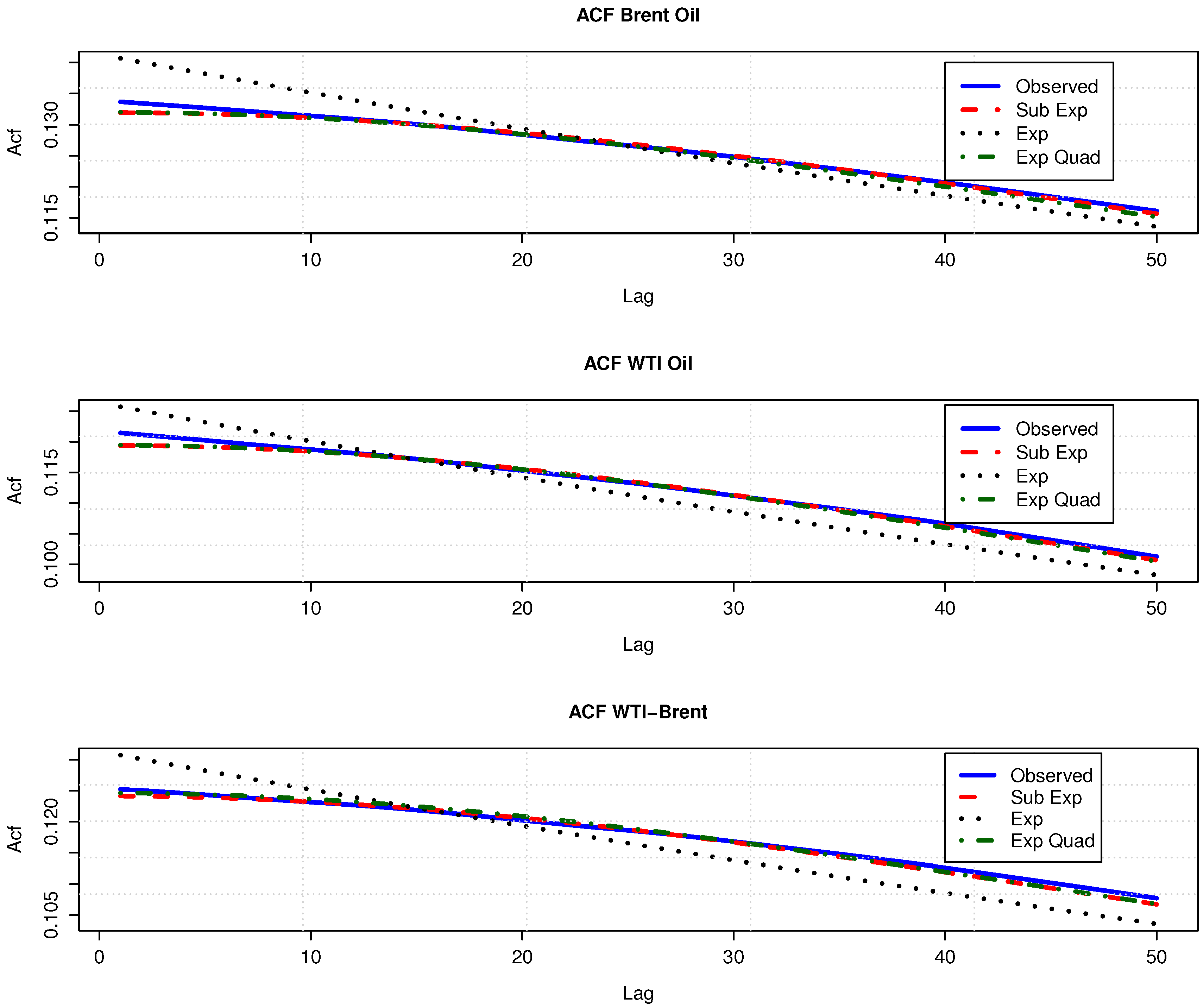
homogeneous fields to empirical covariances. The observed autocovariances are concave decreasing functions, and the exponential model fails to replicate this concavity, particularly in the short term.
Table 5 and Table 6 report calendar spread option prices7 written on the pairs Brent-WTI crude oil and silver-gold. These figures emphasize the impact of a misspecified autocovariance function on the value of calendar spread options. Assuming an OU dynamics for Brent and WTI oil leads to overestimating option values by 5–37% compared to those computed with a sub-exponential covariance. The gap between option prices computed with quadratic exponential and sub-exponential covariances is much smaller and ranges from −1.55–2.95%. For silver against gold, the conclusions are similar: the bias caused by the wrong choice of covariance structure can be significant (up to 6.2% with an OU model and −19.6% with a quadratic exponential covariance). Table 7 presents calendar spread option prices computed by Monte Carlo simulations with different levels of discretization in the space of frequencies. As expected, increasing u n and decreasing the size of the step of discretization reduce the gap between values obtained analytically, as well as the numerical estimates.
To understand the influence of autocorrelation parameters λ k on option values, we perform a sensitivity analysis for the sub-exponential model driven by d = 2 conditional Gaussian fields. Table 8 reports the parameters of this model fitted to Brent and WTI crude oil. We appraise calendar spread exchange options with three sets of autocovariance parameters: λ 1 , λ 2 , λ 1 2 , λ 2 and λ 1 , λ 2 2 . 
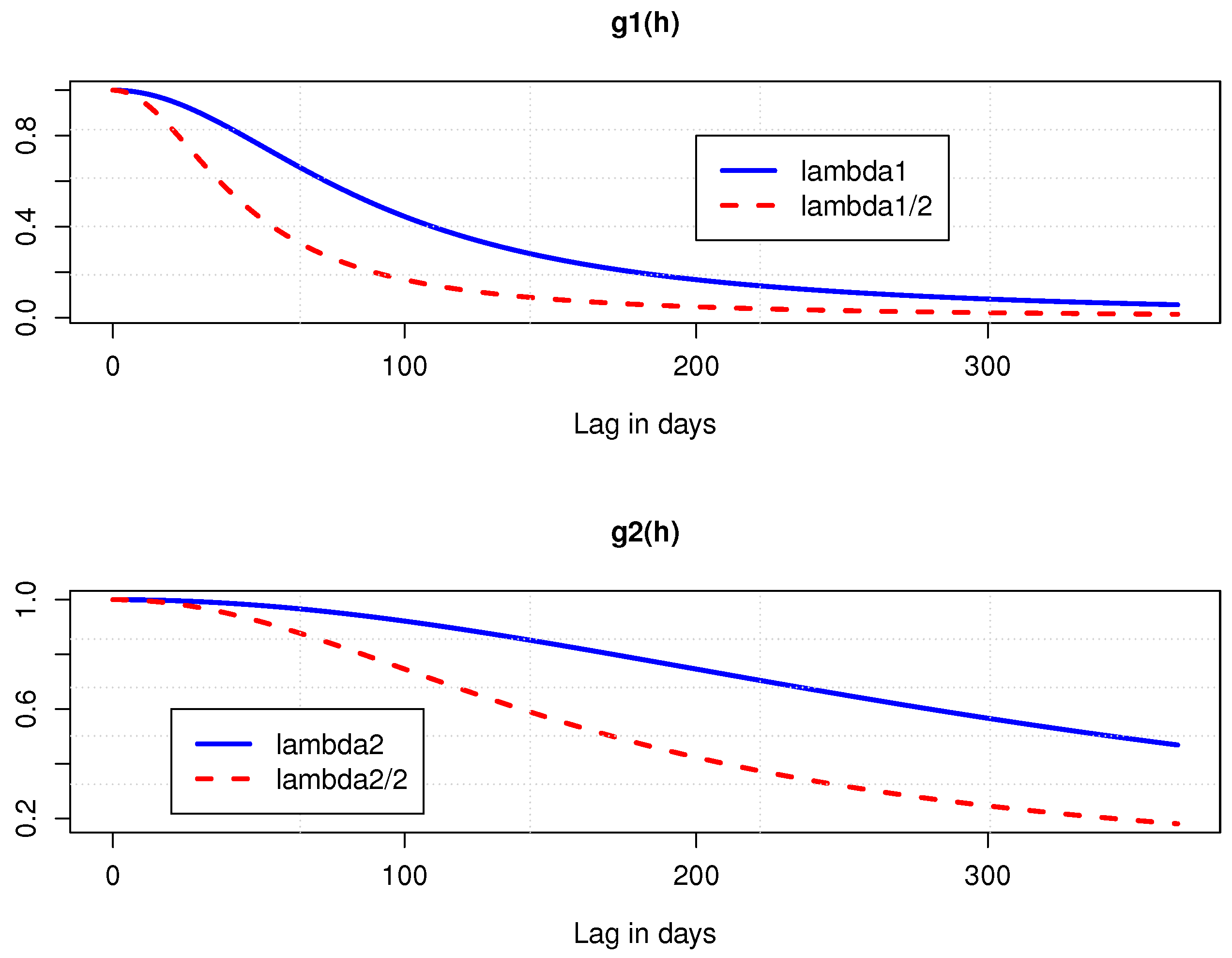
Figure 2 emphasizes the impact of these modifications on autocovariance functions g 1 ( t ) and g 2 ( t ) . We observe that reducing λ 1 or λ 2 decreases the level of autocorrelation of Z t ( 1 ) and Z t ( 2 ) . Table 9 underlines the important role played by λ 1 or λ 2 on option prices. The relative spread between prices computed with λ 1 , λ 2 and λ 1 2 , λ 2 ranges from 5% up to 55%; whereas, the spread between prices obtained with λ 1 , λ 2 and λ 1 , λ 2 2 varies from 7.5–11%. These results confirm the importance of the autocorrelation in the valuation of exotic derivatives like calendar spread exchange options.
Table 10 and Table 11 report Asian calendar spread option prices on Brent vs. WTI crude oil and silver vs. gold. The spreads between prices obtained with sub-exponential and exponential covariance structures are smaller than those of calendar options. However, they remain significant: from −1.84–3.48% for Brent vs. WTI and from −1.74–1.54%. Prices obtained with an exponential quadratic covariance model deviate more widely from those computed with a sub-exponential covariance (from 7.16–20.6%).
To understand the influence of autocovariance parameters λ k on Asian options, we perform a sensitivity analysis for the sub-exponential model driven by d = 2 conditional Gaussian fields. We appraise Asian calendar spread exchange options with the sets of autocovariance parameters, λ 1 , λ 2 , λ 1 2 , λ 2 and λ 1 , λ 2 2 , presented in Table 9. Table 12 reveals that the relative spread between prices computed with λ 1 , λ 2 and λ 1 2 , λ 2 ranges from 0.75–4.3%, whereas the spread between prices obtained with λ 1 , λ 2 and λ 1 , λ 2 2 varies from 0.6–5.5%. The impact of the autocorrelation on Asian option prices is still significant, but less important than for exchange options due to the smoothing induced by the definition of the payoff.

9. Conclusions

This article has two objectives. Firstly, it proposes a simple alternative to models based on Brownian motions that allows for an accurate modeling of covariance and autocorrelation structures. In our approach, price processes are seen as conditional homogeneous Gaussian fields indexed by time. As this field is in general not a semi-martingale, we cannot rely anymore on stochastic calculus to evaluate options. However, a conditional Gaussian field inherits all the properties of the multivariate normal random variable. This guarantees its high analytical tractability.
Homogeneous Gaussian fields indexed by time have a covariance function depending on the lag between two realizations of this field. They include Ornstein–Uhlenbeck processes, and their asymptotic variance and autocovariance are respectively constant and null. The variance of these fields being bounded by a constant, asset yields revert around their mean. This property makes the proposed approach more suitable for the modeling of interest rates or any assets with a mean reverting yield, like commodities.
We study three types of covariance structures with sub-exponential, exponential and hyper- exponential decreasing autocorrelations. We also propose a procedure of simulation based on the spectral decomposition of the covariance matrix. Within this approach, the sample path of simulated prices is known in continuous time. This feature is particularly interesting for the numerical pricing of path-dependent options.
Secondly, we aim to emphasize the importance of the covariance structure in the valuation of calendar spread derivatives. We derive closed form expressions for Asian and non-Asian calendar spread exchange options. Analytical formulas are obtained by the technique of the change of numeraire. Next, we fit models to two pairs of commodities: Brent vs. WTI oil and silver vs. gold. The numerical analysis reveals that these assets exhibit concave decreasing autocovariances that the exponential model fails to replicate. For these asset classes, the best fit is obtained with sub-exponential covariance functions. We observe that covariance misspecification introduces a bias of several percent for the prices of calendar spread exchange options. The numerical illustration emphasizes that assuming an OU dynamics for Brent and WTI oil leads to overestimating option values by 5–37% compared to those computed with a sub-exponential covariance structure. For gold-silver exchange options, the bias introduced by the wrong choice of covariance structure can be significant (up to 6.2% with an OU model and −19.6% with a quadratic exponential covariance). An analysis of the sensitivity of options to a reduction by a half of the autocorrelation factors reveals that prices deviate by 5–55% from their initial values. These results confirm the importance of the autocorrelation in the valuation of calendar exchange options. For Asian options, the spreads between prices obtained with sub-exponential and exponential covariance structures are smaller than those of calendar options. However, they remain significant and range from −1.84–3.48% for Brent vs. WTI and from −1.74–1.54% for gold vs. silver. Prices obtained with an exponential quadratic covariance model deviate more widely from these computed with a sub-exponential covariance (from 7.16–20.6%). An analysis of the sensitivity of options to a reduction by a half of the autocorrelation factors reveals that option values diverge by 0.6–5.5% from their initial price. The impact of the autocorrelation on Asian option prices is still significant, but less important than for exchange options due to the smoothing induced by the definition of the payoff.
There are several interesting topics for future research. For example, it would be interesting to replace constant coefficients in Σ by a time-dependent matrix in order to model the seasonality in dependence modeling. Another improvement could be to model the risk-free rate and/or convenience yield with other Gaussian fields.

Funding

I thank the Chair “Data Analytics and Models for insurance” of BNP Paribas Cardiff, hosted by ISFA (University Claude Bernard, Lyon) and managed by the “Fondation Du Risque”.

Acknowledgments

I acknowledge my colleague Sebastien de Valeriola for his helpful comments and suggestions.

Conflicts of Interest

The author declares no conflict of interest.

Appendix A

Proposition A1.
If the autocovariance functions of X t ( k ) are exponential, C X t ( k ) , X t + h ( k ) = e λ k | h | and if X 0 ( k ) are N ( 0 , 1 ) random variables, then X t ( k ) are Ornstein–Uhlenbeck (OU) processes that obey the following dynamics:
d X t ( k ) = λ k X t ( k ) d t + 2 λ k d W t ( k ) k = 1 , , d ,
where W t ( k ) are d independent Brownian motions.
Proof. 
Let us consider OU processes that are ruled by Equation (A1). We apply Itô’s lemma to the process U t = e λ k t X t ( k ) , then:
d U t = λ k e λ k t X t ( k ) d t e λ k t d X t ( k ) = e λ k t 2 λ k d W t ( k ) ,
and:
U s = U t 2 λ k t s e λ k u d W u ( k ) .
Therefore, we infer that:
X s ( k ) = e λ k ( s t ) X t ( k ) + 2 λ k t s e λ k ( s u ) d W u ( k ) ,
and X 0 ( k ) is distributed according to a Gaussian law, with mean zero and variance equal to one. We have that 2 λ k 0 t e λ k u d W u ( k ) is a normal random of the null mean with variance equal to:
2 λ k 0 t e 2 λ k u d u = 1 e 2 λ k t ,
and e λ k t X 0 ( k ) has a variance equal to e 2 λ k t . The variance of X t ( k ) is then e 2 λ k t + 1 e 2 λ k t = 1; whereas the covariance between X s ( k ) and X t ( k ) is equal to:
C X s ( k ) , X t ( k ) = 2 λ k E 0 s e λ k ( s u ) d W u ( k ) 0 t e λ k ( t u ) d W u ( k ) + e λ k ( t + s ) = 2 λ k e λ k ( s + t ) E 0 s t e λ k u d W u ( k ) 2 | F 0 + e λ k ( t + s ) = 2 λ k e λ k ( s + t ) 1 2 λ k e 2 λ k s t 1 + e λ k ( t + s ) = e λ k | s t | .
Notice that in this article, we set X 0 ( k ) = 0 and define the Gaussian field by its conditional covariance to F 0 . The covariance between Z t ( k ) = X t ( k ) | X 0 ( k ) = 0 and Z s ( k ) = X s ( k ) | X 0 ( k ) = 0 is then:
C Z t ( k ) , Z t + h ( k ) = g k ( s t ) g k ( s ) g k ( t ) = e λ k | s t | e λ k ( s + t ) .

Appendix B. Detailed Proofs

Proof of Proposition 2.
Given that W 1 and W 2 are independent and that the expectation of the integral with respect to a μ -noise is null, we have the following relation:
E X s X t = E R + cos u s W 1 ( d u ) + R + sin u s W 2 ( d u ) × R + cos u t W 1 ( d u ) + R + sin u t W 2 ( d u ) = E R + cos u s W 1 ( d u ) R + cos u t W 1 ( d u ) + E R + sin u s W 2 ( d u ) R + sin u t W 2 ( d u ) .
As E W k ( φ ) W k ( ψ ) ¯ = R φ ( t ) ψ ( t ) ¯ μ ( d t ) , for k = 1 , 2 , we infer that:
E X s X t = R + cos u s cos u t + sin u s sin u t μ ( d u ) = R + cos u s cos u t sin u s sin u t μ ( d u ) = R + cos u ( s t ) μ ( d u ) .
Proof of Proposition 3.
For all ω C , if we remember the definition (16) of the change of the measure from Q to Q S 2 , we can develop the moment generating function as follows:
E Q S 2 e ω R t , T | F 0 = e ω r T t + c 1 T c 2 t ω α 1 ( T ) + ω 1 α 2 ( t ) × E e ω Σ 1 , . Z T ω 1 Σ 2 , . Z t | F 0 E e α 2 ( t ) + Σ 2 , : Z t | F 0 .
By construction, the expectation in the denominator is equal to one. The variance of Σ 1 , . Z T and Σ 2 , . Z t is respectively equal to k = 1 d σ 1 k 2 1 g k ( T ) 2 and k = 1 d σ 2 k 2 1 g k ( t ) 2 . Their covariance is equal to:
C Σ 1 , . Z T , Σ 2 , . Z t | F 0 = k = 1 d σ 1 k σ 2 k g k ( T t ) g k ( T ) g k ( t ) .
Then, the difference ω Σ 1 , . Z T ω 1 Σ 2 , . Z t is a normal random variable with a null mean and a variance equal to:
v ( ω , t , T ) 2 = ω 2 k = 1 d σ 1 k 2 1 g k ( T ) 2 + ω 1 2 k = 1 d σ 2 k 2 1 g k ( t ) 2 2 ω ω 1 k = 1 d σ 1 k σ 2 k g k ( T t ) g k ( T ) g k ( t ) .
After simplification, we get that:
v ( ω , t , T ) 2 = 2 ω 2 α 1 ( T ) + 2 ω 1 2 α 2 ( t ) 2 ω ω 1 k = 1 d σ 1 k σ 2 k g k ( T t ) g k ( T ) g k ( t ) .
The expectation in the numerator of Equation (A2) is the expectation of a lognormal random variable, and the moment generating function (mgf) of R t , T is then equal to:
E Q S 2 e ω R t , T | F 0 = exp ω r T t + c 1 T c 2 t ω α 1 ( T ) + ω 1 α 2 ( t ) + 1 2 v ( ω , t , T ) 2 .
From this last equation, we infer that R t , T is a normal random variable of parameters μ R ( t , T ) and σ R ( t , T ) . ☐
Proof of Proposition 4.
If we rewrite the option price as an expectation under the measure Q S 2 , we obtain that:
E Q S 2 β 1 β 2 S 0 ( 1 ) S 0 ( 2 ) e R t , T 1 + | F 0 = β 1 β 2 S 0 ( 1 ) S 0 ( 2 ) u m i n + e u f R t , T ( u ) d u u m i n + f R t , T ( u ) d u .
where u m i n = ln β 2 β 1 S 0 ( 2 ) S 0 ( 1 ) . According to the definition (19) of d 2 , the integral in the first term is equal to:
u m i n + f R t , T ( u ) d u = Φ d 2 ( t , T ) ;
whereas the second integral of Equation (A4) is developed as follows:
u m i n + e u f R t , T ( u ) d u = 1 2 π σ R u m i n + exp 1 2 u 2 2 u μ R + σ R 2 + μ R 2 σ R 2 d u .
If we define a new variable v = μ R + σ R 2 , we develop this last equation as:
u m i n + e u f R t , T ( u ) d u = exp μ R + 1 2 σ R 2 2 π σ R u m i n + exp 1 2 u v 2 σ R 2 d u = exp μ R + 1 2 σ R 2 Φ d 1 ( t , T ) .
Finally, combining Equations (A4)–(A6) leads to the following result:
E Q S 2 β 1 β 2 S T ( 1 ) S t ( 2 ) 1 + | F 0 = β 1 β 2 S 0 ( 1 ) S 0 ( 2 ) exp μ R + 1 2 σ R 2 Φ d 1 ( t , T ) Φ d 2 ( t , T ) .
Given that μ R ( t , T ) r ( T t ) + c 2 t + 1 2 σ R ( t , T ) 2 = c 1 T , we can conclude the proof. ☐
Proof of Proposition 5.
For a sub-exponential covariance function, the double integral 0 t 0 T g k ( u v ) d v d u is equal to 0 t 0 T λ k 2 λ k 2 + ( u v ) 2 d u d v . On the other hand, the first integral is equal to:
0 T λ k 2 λ k 2 + ( u v ) 2 d u = λ k tan 1 v λ k λ k tan 1 v T λ k .
The integral of the arctangent function is given by:
tan 1 ( x ) d x = x tan 1 ( x ) 1 2 ln ( 1 + x 2 ) + C .
Therefore, we infer the following result:
0 t 0 T g r ( u v ) d u d v = λ k 0 t tan 1 v λ k d v λ k 0 t tan 1 v T λ k d v = λ k 2 0 t λ k tan 1 s d s λ k 2 T λ k t T λ k tan 1 s d s .
Furthermore, we also have that:
λ k 2 0 t λ k tan 1 s d s = t λ k tan 1 t λ k 1 2 λ k 2 ln 1 + t 2 λ k 2
and:
λ k 2 T λ k t T λ k tan 1 s d s = λ k 2 x tan 1 ( x ) 1 2 ln ( 1 + x 2 ) x = T λ k x = t T λ k ,
from which we obtain the expression (23). On the other hand, by direct integration, we can show that:
0 t 0 T g k ( u ) g k ( v ) d v d u = 0 t λ k 2 λ k 2 + v 2 d v 0 T λ k 2 λ k 2 + u 2 d u = λ k 2 arctan t λ k arctan T λ k .
Proof of Proposition 7.
By the definition of α j ( t ) , we have that:
1 t 0 t α j ( s ) d s = 1 2 1 t k = 1 d σ j k 2 t 0 t g k ( s ) 2 d s
and:
0 t g k ( s ) 2 d s = 0 t λ k 4 λ k 2 + s 2 2 d s = λ k 2 tan 1 t λ k + λ k 2 t 2 t 2 + λ k 2 .
Therefore, we can conclude the proof. ☐
Proof of Proposition 8.
The double integral 0 t 0 T g k ( u v ) d v d u is developed as follows:
0 t 0 T g k ( u v ) d v d u = 0 t 0 T e λ k | u v | d v d u = 0 t 0 t e λ k | u v | d v d u + 0 t t T e λ k | u v | d v d u .
On the other hand, the first integral is equal to:
0 t 0 t e λ k | u v | d v d u = 2 t λ 1 λ 2 1 e λ t ,
and the second integral is equal to:
0 t t T e λ k | u v | d v d u = 0 t t T e λ k ( u v ) d v d u = 1 λ k 2 1 e λ k t e λ k ( t T ) + e λ k T .
Combining Equations (A7)–(A9) allows us to obtain Equation (26). Furthermore, we deduce by direct integration that:
0 t 0 T g k ( u ) g k ( v ) d v d u = 0 t e λ k v d v 0 T e λ k u d u = 1 λ k 2 1 e λ k t 1 e λ k T .
Proof of Proposition 11.
The double integral 0 t 0 T g k ( u v ) d v d u is equal to:
0 t 0 T g k ( u v ) d v d u = 0 t 0 T e 1 4 λ k u v 2 d v d u .
We may check that the inner integral is given by:
0 T e 1 4 λ k u v 2 d v = π λ k erf u 2 λ k erf u T 2 λ k .
Furthermore, the integral of the first error function in this last equation is equal to:
0 t erf u 2 λ k d u = t erf t 2 λ k 2 λ k π 1 e t 2 4 λ k .
The second integral present in Equation (A10) is equal to:
0 t erf u T 2 λ k d x = ( T t ) erf T t 2 λ k T erf T 2 λ k + λ k π 2 e t T 2 4 λ k e T 2 4 λ k .
Combining Equations (A10)–(A12) allows us to obtain Equation (29). As we have that:
0 t 0 T g k ( u ) g k ( v ) d v d u = 0 t e v 2 4 λ k d v 0 T e u 2 4 λ k d u = π λ k erf t 2 λ k erf T 2 λ k ,
we can conclude the proof. ☐
Proof of Proposition 13.
By the definition of α j ( s ) , we have that:
1 t 0 t α j ( s ) d s = 1 2 1 t k = 1 d σ j k 2 t 0 t e h 2 2 λ k d s .
Given that:
0 t e h 2 2 λ k d s = π λ k 2 erf t 2 λ k ,
we can conclude the proof. ☐
Proof of Proposition 14.
Let ω C . By the definition of the change of measure (16), the moment generating function (mgf) of G T ( 1 ) G t ( 2 ) is developed as follows:
E Q G 2 e ω A t , T | F 0 = e ω 1 2 r T t + ω 1 2 c 1 T c 2 t ω T 0 T α 1 ( s ) d s + ω t 0 t α 2 ( s ) d s × E Q G 2 e ω 1 T Σ 1 , . 0 T Z s d s 1 t Σ 2 , . 0 t Z s d s | F 0 = e ω 1 2 r T t + ω 1 2 c 1 T c 2 t ω T 0 T α 1 ( s ) d s + ω t 0 t α 2 ( s ) d s 1 2 σ ln G 2 ( t ) 2 × E e ω 1 T Σ 1 , . 0 T Z s d s ω 1 1 t Σ 2 , . 0 t Z s d s | F 0 .
The variances of 1 T Σ 1 , . 0 T Z s d s and 1 t Σ 2 , . 0 t Z s d s are respectively σ ln G 1 ( T ) 2 and σ ln G 2 ( t ) 2 , as defined by Equation (25). The weighted sum of random field integrals has a covariance equal to:
C 1 T Σ 1 , . 0 T Z s d s , 1 t Σ 2 , . 0 t Z s d s | F 0 = 1 T t C Σ 1 , . 0 T Z s d s , Σ 2 , . 0 t Z s d s | F 0 = 1 T t k = 1 d σ 1 k σ 2 k 0 t 0 T g k ( u v ) g k ( u ) g k ( v ) d v d u .
The random variable ω 1 T Σ 1 , . 0 T Z s d s ω 1 1 t Σ 2 , . 0 t Z s d s is then normal, with a null mean and a variance equal to:
v ( ω ) 2 = ω 2 σ ln G 1 ( T ) 2 + ω 1 2 σ ln G 2 ( t ) 2 2 ω ω 1 T t × k = 1 d σ 1 k σ 2 k 0 t 0 T g k ( u v ) g k ( u ) g k ( v ) d v d u
and we can conclude that the mgf of A t , T with t T under the measure Q G 2 is:
E Q G 2 e ω A t , T | F 0 = exp ω 1 2 r T t + ω 1 2 c 1 T c 2 t ω T 0 T α 1 ( s ) d s + ω t 0 t α 2 ( s ) d s × exp 1 2 σ ln G 2 ( t ) 2 + 1 2 v ( ω ) 2 .
After simplification, we obtain Equations (34) and (35). ☐
Proof of Proposition 15.
Using a change of numeraire allows us to rewrite the option price as follows:
e r T E ( β 1 G T ( 1 ) β 2 G t ( 2 ) ) + | F 0 = β 2 e r T exp 1 2 r + c 2 t 1 t 0 t α 2 ( s ) d s + 1 2 σ ln G 2 ( t ) 2 × E Q G 2 β 1 β 2 G T ( 1 ) G t ( 2 ) 1 + | F 0 .
If f A ( u ) denotes the density of A t , T under the measure Q G 2 , the expectation in this last equation is given by:
E Q G 2 β 1 β 2 G T ( 1 ) G t ( 2 ) 1 + | F 0 = ln β 2 β 1 β 1 β 2 e u 1 f A ( u ) d u .
As A t , T is normal and by the definition of d 2 ( t , T ) , the second integral is equal to:
ln β 2 β 1 f A ( u ) d u = Φ d 2 ( t , T ) ,
whereas the first integral is rewritten after a change of variable as follows:
β 1 β 2 ln β 2 β 1 e u f A ( u ) d u . = β 1 β 2 exp μ A + 1 2 σ A 2 Φ d 1 ( t , T ) .
Finally:
E Q G 2 β 1 β 2 e A t , T 1 + | F 0 = β 1 β 2 exp μ A + 1 2 σ A 2 Φ d 1 ( t , T ) Φ d 2 ( t , T ) .
Combining Equations (A15)–(A16) leads to the following expression for the Asian exchange calendar option:
e r T E ( β 1 G T ( 1 ) β 2 G t ( 2 ) ) + | F 0 = β 2 e r T exp 1 2 r + c 2 t 1 t 0 t α 2 ( s ) d s + 1 2 σ ln G 2 ( t ) 2 × β 1 β 2 exp μ A + 1 2 σ A 2 Φ d 1 ( t , T ) Φ d 2 ( t , T ) .

References

  1. Adler, Robert J. 1981. The Geometry of Random Fields. Chichester: John Wiley. [Google Scholar]
  2. Adler, Robert J., and Jonathan E. Taylor. 2007. Random Fields and Geometry. New York: Springer. [Google Scholar]
  3. Adler, Robert J., and Jonathan E. Taylor. 2009. Topological Complexity of Smooth Random Fields Functions: Ecole d’ete de Probabilite de Saint-Flour. Berlin/Heidelberg: Springer, pp. 13–35. Available online: https://www.springer.com/gb/book/9783642195792 (accessed on 7 August 2018).
  4. Bender, Christian, Tommi Sottinen, and Esko Valkeila. 2006. Arbitrage with fractional Brownian motion? Theory of Stochastic Processes 12: 23–34. [Google Scholar]
  5. Bessembinder, Hendrik, Jay F. Coughenour, Paul J. Seguin, and Margaret Monroe Smoller. 1995. Mean reversion in equilibrium asset prices: Evidence from the futures term structure. Journal of Finance 50: 361–75. [Google Scholar] [CrossRef]
  6. Biagini, Francesca, Camila Botero, and Irene Schreiber. 2017. Risk-minimization for life insurance liabilities with dependent mortality risk. Mathematical Finance 27: 505–33. [Google Scholar] [CrossRef]
  7. Biffis, Enrico, and Pietro Millossovich. 2006. A bidimensional approach to mortality risk. Decisions in Economics and Finance 29: 71–94. [Google Scholar] [CrossRef]
  8. Bochner, Salomon. 1933. Monotone Funktionen, Stieltjessche Integrale und harmonische Analyse. Mathematische Annalen 108: 378–410. [Google Scholar] [CrossRef]
  9. Cheridito, Patrick. 2003. Arbitrage in fractional Brownian motion models. Finance and Stochastics 7: 533–53. [Google Scholar] [CrossRef]
  10. Cortazar, Gonzalo, and Eduardo S. Schwartz. 1994. The valuation of commodity contingent claims. The Journal of Derivatives 1: 27–29. [Google Scholar] [CrossRef]
  11. Cressie, Noel A. C. 1993. Statistics for Spatial Data, 2nd ed. New York: John Wiley & Sons. [Google Scholar]
  12. Goldstein, Robert S. 2000. The term structure of interest rates as a random field. The Review of Financial Studies 13: 365–84. [Google Scholar] [CrossRef]
  13. Gibson, Rajna, and Eduardo S. Schwartz. 1990. Stochastic convenience yield and the pricing of oil contingent claims. The Journal of Finance 45: 959–76. [Google Scholar] [CrossRef]
  14. Hainaut, Donatien. 2017. Continuous mixed-Laplace jump diffusion models for stocks and commodities. Quantitative Finance and Economics 1: 145–73. [Google Scholar] [CrossRef]
  15. Kennedy, Douglas P. 1994. The term structure of interest rates as a Gaussian random field. Mathematical Finance 4: 257–58. [Google Scholar] [CrossRef]
  16. Kimmel, Robert L. 2004. Modeling the term structure of interest rates: a new approach. Journal of Financial Economics 72: 143–83. [Google Scholar] [CrossRef]
  17. Margrabe, William. 1978. The Value of an Option to Exchange One Asset for Another. Journal of Finance 33: 177–86. [Google Scholar] [CrossRef]
  18. Matern, Bertil. 1986. Spatial Variation. Lecture Notes in Statistics. Berlin: Springer. [Google Scholar]
  19. Ozkan, Fehmi, and Thorsten Schmidt. 2009. Credit risk with infinite dimensional Lévy processes. Statistics & Decisions 23: 281–99. [Google Scholar]
  20. Schwartz, Eduardo. 1997. The stochastic behavior of commodity prices: implications for valuation and hedging. Journal of Finance 52: 923–73. [Google Scholar] [CrossRef]
  21. Willinger, Walter, Murad S. Taqqu, and Vadim Teverovsky. 1999. Stock market prices and long-range dependence. Finance and Stochastics 3: 1–13. [Google Scholar] [CrossRef]
  22. Wu, Ruhao. 2016. Gaussian Process and Functional Data Methods for Mortality Modeling. Ph.D. Dissertation, University of Leicester, Leicester, UK. [Google Scholar]
1
Excepting the Ornstein Uhlenbeck process, that is a Markov process that may be reformulated as an homogeneous Gaussian field. However, in general, a time Gaussian field is not a Markov process.
2
The yield y t ( j ) is here defined by the cumulative return up to time t of the j t h asset.
3
WE remark that Σ may eventually be replaced by a time-dependent matrix Σ ( t ) in order to replicate seasonality effects in the covariance. In this framework, the pricing by simulations would still be possible.
4
Notice that the same problem arises for models based on fractional Brownian motions, which are not arbitrage free (see, e.g., Cheridito (2003) and Bender et al. (2006).
5
Notice that ν ( . ) can be any measure on R , of probability or not (e.g., Lebesgue measure).
6
As mentioned in Section 2, homogeneous fields have constant asymptotic variance. This feature makes them more suitable for the modeling of commodities or interest rates.
7
The discount rate is set to r = 5 % and c 1 = c 2 = 0 .
Figure 1. Plot of the autocovariance functions (ACF) of Brent and WTI oil log-returns. Time lags are expressed in days. “Observed”: empirical covariances. “Sub Exp”, “Exp” and “Exp quad”: sub exponental, exponential and quadratric exponential modeled covariances.
Risks 06 00077 g001
Figure 2. Plot of sub-exponential covariance functions g 1 ( t ) and g 2 ( t ) for the model fitted to Brent and WTI oil log-returns with d = 2 . Parameters λ 1 and λ 2 are reported in Table 8.
Risks 06 00077 g002
Table 1. Square root errors: Brent vs. WTI oil. Number of lags: 150 days.
d g k ( h ) = λ k 2 λ k 2 + h 2 g k ( h ) = e λ k | h | g k ( h ) = e λ k h 2
10.06690.05670.0943
20.00940.04550.0137
30.00850.04510.0121
40.00510.04500.0101
Table 2. Square root errors: silver vs. gold. Number of lags: 150 days.
d g k ( h ) = λ k 2 λ k 2 + h 2 g k ( h ) = e λ k | h | g k ( h ) = e λ k h 2
10.05370.04830.0540
20.01890.01540.0268
30.00670.01340.0211
40.00460.01330.0205
Table 3. Model parameters: Brent vs. WTI oil. Number of lags: 150 days and d = 3 .
Sub-Exponential
k λ k σ 1 , k σ 2 , k
10.18870.15460.1778
20.36140.25020.2477
32.24820.21320.1626
Exponential
k λ k σ 1 , k σ 2 , k
10.1000.14280.08124
21.4540.21300.18387
32.1460.27490.29315
Quadratic Exponential
k λ k σ 1 , k σ 2 , k
11.8440.317370.2776
217.1020.090770.1352
330.6380.150330.1542
Table 4. Model parameters: silver vs. gold. Number of lags: 150 days and d = 3 .
Sub-Exponential
k λ k σ 1 , k σ 2 , k
10.20910.14860.0374
20.26360.00210.0784
30.99220.28190.1705
Exponential
k λ k σ 1 , k σ 2 , k
10.21310.08040.0560
20.70880.27720.1840
31.89220.14750.0005
Quadratic Exponential
k λ k σ 1 , k σ 2 , k
10.81510.25690.1793
24.03570.16540.0198
340.61570.08550.0615
Table 5. S t ( 1 ) : Brent, S t ( 2 ) : WTI. d = 3 . Option payoff: ( β 1 S T ( 1 ) β 2 S t ( 2 ) ) + where T = 1 year and t ranges from 0.3–0.9 years. β 1 and β 2 are such that β 1 S 0 ( 1 ) = β 2 S 0 ( 2 ) = 1 .
Calendar Spread Exchange Options
t SubExpRelative Error (%)Exp QuadRelative Error (%)
ExpExp vs. Sub ExpExp Quad vs. Sub Exp
0.30.164760.173425.2510.16600.7250
0.40.161840.168814.3030.1604−0.9173
0.50.155020.161163.9550.1526−1.5519
0.60.144170.150354.2830.1422−1.3608
0.70.127760.135696.2120.1265−0.9992
0.80.102430.1155612.8100.1023−0.1369
0.90.062360.0856437.3440.06422.9498
Table 6. S t ( 1 ) : Silver, S t ( 2 ) : gold. d = 3 . Option payoff: ( β 1 S T ( 1 ) β 2 S t ( 2 ) ) + where T = 1 year and t ranges from 0.3–0.9 years. β 1 and β 2 are such that β 1 S 0 ( 1 ) = β 2 S 0 ( 2 ) = 1 .
Calendar Spread Exchange Options
t SubExpRelative Error (%)Exp QuadRelative Error (%)
ExpExp vs. Sub ExpExp Quad vs. Sub Exp
0.30.122710.12251−0.1630.124941.821
0.40.116130.116700.4920.116330.170
0.50.108740.110351.4830.10661−1.957
0.60.100670.103392.6930.09570−4.942
0.70.092020.095714.0110.08357−9.178
0.80.082740.087185.3680.07065−14.614
0.90.073050.077586.2000.05875−19.574
Table 7. S t ( 1 ) : Brent, S t ( 2 ) : WTI. d = 3 . Option payoff: ( β 1 S T ( 1 ) β 2 S t ( 2 ) ) + where T = 1 year and t equals 0.4 years. β 1 and β 2 are such that β 1 S 0 ( 1 ) = β 2 S 0 ( 2 ) = 1 . Prices are obtained with 10,000 simulations.
Monte-Carlo Simulations
u n u j + 1 u j Sub ExpExpExp Quad
400.300.15540.15630.1585
0.250.16190.16060.1582
0.200.15980.16300.1594
0.150.16170.16210.1616
0.100.15970.16540.1596
0.050.16030.16510.1618
500.300.15370.16430.1610
0.250.15880.16280.1577
0.200.16380.16790.1584
0.150.15900.16270.1569
0.100.16310.16730.1556
0.050.16290.16830.1578
Analytical price0.16180.16880.1604
Table 8. Model parameters: Brent vs. WTI oil. Number of lags: 150 days and d = 2 . The last columns contain values of λ k used to test the sensitivity of option prices to autocovariance parameters.
Sub-Exponential Parameters for the Sensitivity Analysis
k σ 1 , k σ 2 , k λ 1 , λ 2 λ 1 2 , λ 2 λ 1 , λ 2 2
10.24750.26550.24510.12260.2451
20.27010.21490.93930.93930.4696
Table 9. S t ( 1 ) : Brent, S t ( 2 ) : WTI. d = 2 . Option payoff: ( β 1 S T ( 1 ) β 2 S t ( 2 ) ) + where T = 1 year and t ranges from 0.3–0.9 years. β 1 and β 2 are such that β 1 S 0 ( 1 ) = β 2 S 0 ( 2 ) = 1 .
Sensitivity of Calendar Spread Exchange Options to Autocovariance Parameters
t PricePriceRelative Spread (%)PriceRelative Spread (%)
λ 1 , λ 2 λ 1 2 , λ 2 λ 1 2 , λ 2 vs. λ 1 , λ 2 λ 1 , λ 2 2 λ 1 , λ 2 2 vs. λ 1 , λ 2
0.30.168280.177085.2270.183358.956
0.50.155470.165536.4730.1726811.072
0.70.128140.1485115.8950.1416510.540
0.90.063160.0978354.9050.067937.564
Table 10. S t ( 1 ) : Brent, S t ( 2 ) : WTI. d = 3 . Option payoff: ( β 1 G T ( 1 ) G 2 S t ( 2 ) ) + where T = 1 year and t ranges from 0.3–0.9 years. β 1 = β 2 = 1 .
Asian Calendar Spread Exchange Options
t Sub ExpExpRelative Error (%)Exp QuadRelative Error (%)
Exp vs. Sub ExpExp Quad vs. Sub Exp
0.30.064060.066293.4770.068657.162
0.40.057970.058631.1430.062247.368
0.50.050590.05039−0.3920.054407.530
0.60.042280.04170−1.3770.045657.960
0.70.033310.03270−1.8450.036379.188
0.80.023930.02360−1.3840.0268712.314
0.90.014700.015042.3060.0177320.600
Table 11. S t ( 1 ) : Silver, S t ( 2 ) : gold. d = 3 . Option payoff: ( β 1 G T ( 1 ) G 2 S t ( 2 ) ) + where T = 1 year and t ranges from 0.3–0.9 years. β 1 = β 2 = 1 .
Asian Calendar Spread Exchange Options
t Sub ExpExpRelative Error (%)Exp QuadRelative Error (%)
Exp vs. Sub ExpExp Quad vs. Sub Exp
0.30.060440.05984−0.9840.064086.024
0.40.056280.05537−1.6050.057872.828
0.50.052070.05116−1.7430.05175−0.607
0.60.047960.04726−1.4470.04586−4.376
0.70.044090.04376−0.7610.04036−8.474
0.80.040620.040730.2640.03547−12.687
0.90.037680.038261.5400.03146−16.505
Table 12. S t ( 1 ) : Brent, S t ( 2 ) : WTI. d = 2 . Option payoff: ( β 1 G T ( 1 ) G 2 S t ( 2 ) ) + where T = 1 year and t ranges from 0.3–0.9 years. β 1 = β 2 = 1 .
Sensitivity of Asian Calendar Spread Exchange Options to Autocovariance Parameters
t PricePriceRelative Spread (%)PriceRelative Spread (%)
λ 1 , λ 2 λ 1 2 , λ 2 λ 1 2 , λ 2 vs. λ 1 , λ 2 λ 1 , λ 2 2 λ 1 , λ 2 2 vs. λ 1 , λ 2
0.30.067810.069953.1470.071245.0538
0.50.053690.054100.7540.056134.5379
0.70.036070.036691.7140.037122.9144
0.90.017980.018764.3750.018090.6626

