Log-Normal or Over-Dispersed Poisson?


Department of Economics, University of Oxford & Oriel College, Oxford OX1 4EW, UK
Risks 2018, 6(3), 70; https://doi.org/10.3390/risks6030070
Submission received: 18 June 2018
/
Revised: 5 July 2018
/
Accepted: 6 July 2018
/
Published: 9 July 2018
Abstract
Although both over-dispersed Poisson and log-normal chain-ladder models are popular in claim reserving, it is not obvious when to choose which model. Yet, the two models are obviously different. While the over-dispersed Poisson model imposes the variance to mean ratio to be common across the array, the log-normal model assumes the same for the standard deviation to mean ratio. Leveraging this insight, we propose a test that has the power to distinguish between the two models. The theory is asymptotic, but it does not build on a large size of the array and, instead, makes use of information accumulating within the cells. The test has a non-standard asymptotic distribution; however, saddle point approximations are available. We show in a simulation study that these approximations are accurate and that the test performs well in finite samples and has high power.
1. Introduction
Which is the better chain-ladder model for claim reserving: over-dispersed Poisson or log-normal? While the expert may have a go-to model, the answer should be informed by the data. Choosing the wrong model could substantially influence the quality of the reserve forecast. Yet, so far, no statistical theory is available that supports the actuary in his/her decision and that allows him/her to make a solid argument in favour of either model.
We develop a test that can distinguish between over-dispersed Poisson and log-normal data generating processes, both of which have a long history in claim reserving. The test exploits that the former model fixes the variance to mean ratio across the array, while the latter assumes a common standard deviation to mean ratio. Consequently, the test statistic is based on estimators for the variation in the respective models. The idea is drawn from the econometric literature on encompassing. Intuitively, the test asks whether the null-model can accurately predict the behaviour of the rival model’s variation estimator when the null-model is true.
The over-dispersed Poisson model is appealing since it naturally pairs with Poisson quasi-likelihood estimation, replicating the popular chain-ladder technique in run-off triangles (Kremer 1985, pp. 130). Furthermore, this model makes for an appealing story due to its relation to compound Poisson distributions. Such distributions give the aggregate incremental claims an interpretation as the sum over a Poisson number of claims with random individual claim amounts (Beard et al. 1984, Section 3.2). A popular method to generate distribution forecasts for the over-dispersed Poisson model is bootstrapping (England and Verrall 1999; England 2002). While in widespread use, there is so far no theory proving the validity of the bootstrap in this setting. Furthermore, in some settings, the method seems to produce unsatisfactory results.
Recently, Harnau and Nielsen (2017) developed a theory that gives the over-dispersed Poisson model a rigorous statistical footing. They propose an asymptotic framework based on infinitely-divisible distributions that keeps the dimension of the data array fixed and instead builds on large cell means. This resolves the incidental parameter problem (Lancaster 2000; Neyman and Scott 1948) that renders a standard asymptotic theory based on a large array invalid and arises since the number of parameters grows with the size of the array. The class of infinitely-divisible distributions includes compound Poisson distributions, which are appealing in an insurance context, as noted above. We can then interpret large cell means as the result of a large latent underlying number of claims. Other infinitely-divisible distributions that can be reconciled with the over-dispersed Poisson structure include Poisson, gamma and negative binomial.
The intuition for the theory by Harnau and Nielsen (2017) is that the array is roughly normally distributed for large cell means, so that the results remind us of a classical analysis of variance (ANOVA) setting. Harnau and Nielsen (2017) show that Poisson quasi-likelihood estimators are t-distributed, and F-tests based on Poisson likelihoods can be used to test for model reduction, such as for the absence of a calendar effect. Finally, chain-ladder forecast errors are t-distributed, giving rise to closed-form distribution forecasts including for aggregates, such as the reserve or cash-flow. In their simulations, Harnau and Nielsen (2017) find that while the bootstrap (England and Verrall 1999; England 2002) matches the true forecast error distribution better on average, the t-forecast produces fewer outliers and appears more robust.
Building on the asymptotic framework put forward by Harnau and Nielsen (2017), Harnau (2018a) proposes misspecification tests for two crucial assumptions of the over-dispersed Poisson model. First, the variance to mean ratio is assumed to be common across the array. Second, accident effects are not allowed to vary over development years and vice versa. To check for a violation of these assumptions, Harnau (2018a) suggests splitting the run-off triangle into sub-samples and then testing whether a reduction from individual models for each sub-sample to a single model for the full array can be justified. While the idea of splitting the sample is borrowed from time-series econometrics (Chow 1960), the theory for a reduction to a single model is again reminiscent of an ANOVA setting. A classical Bartlett test (Bartlett 1937) can be used to assess whether we can justify common variance to mean ratios. This is followed by an independent F-test for the absence of breaks in accident and development effects. Again, the asymptotics needed to arrive at these results keep the dimension of the array fixed, growing instead the cell means. Harnau (2018a) also shows that these misspecification tests can be used in a similar fashion in a finite sample log-normal model.
The log-normal model introduced by Kremer (1982), who relates it to the ANOVA literature, features a predictor structure that is reminiscent of the classical chain-ladder. Verrall (1994) refers to this as the chain-ladder linear model, while Kuang et al. (2015) use the term geometric chain-ladder. The latter authors show that the maximum likelihood estimators in the log-normal model can be interpreted as development factors of geometric averages, compared to an interpretation of arithmetic averages arising for the classical chain-ladder. An advantage of the log-normal model is that an exact Gaussian distribution theory applies to the maximum likelihood estimators. However, since these estimators are computed on the log scale, a bias is introduced on the original scale. Verrall (1991) tackles this issue and derives unbiased estimators for the mean and standard deviation on the original scale. One issue for full distribution forecasts in the log-normal model is that the insurer is usually not interested in forecasts for individual cells, but rather for cell sums such as the reserve or the cash-flow. However, the log-normal distribution is not closed under convolution, so that cell sums are not log-normally distributed.
Recently, Kuang and Nielsen (2018) proposed a theory that includes closed-form distribution forecasts for cell sums, such as the reserve, in the log-normal model, thus remedying one of its drawbacks. Kuang and Nielsen (2018) combined the insight by Thorin (1977) that the log-normal distribution is infinitely divisible and the asymptotic framework by Harnau and Nielsen (2017). Based on this, they propose a theory for generalized log-normal models, a class that nests the log-normal model, but is not limited to it. In particular, the distribution is not assumed to be exactly log-normal, but merely needs to be infinitely divisible with a moment structure close to that of the log-normal model. The asymptotics in this framework again leave the dimension of the array untouched to avoid an incidental parameter problem. In contrast to the theory for large cell means in the over-dispersed Poisson model, results are now for small standard deviation to mean ratios.
For the generalized log-normal model, Kuang and Nielsen (2018) show that least squares estimators computed on the log scale are asymptotically t-distributed, and simple F-tests based on the residual sum of squares can be used to test for model reduction. Reassuringly, these results match the exact results in a log-normal model. Beyond that, they also prove that forecast errors on the original scale are asymptotically t-distributed so that distribution forecasting for cell sums is straightforward. Further, they show that the misspecification tests by Harnau (2018a) are asymptotically valid for the generalized log-normal model, just as they were in finite samples for the log-normal model.
We remark that besides over-dispersed Poisson and log-normal models, there exist a number of reserving models that we do not consider further in this paper. England and Verrall (2002) give an excellent overview. Perhaps the most popular contender is the “distribution-free” model by Mack (1993). This model also replicates the classical chain-ladder, but differs from the over-dispersed Poisson model. Mack (1993) derives the expression for forecast standard errors. However, so far, no full distribution theory exists for this model.
With a range of theoretical results in place for over-dispersed Poisson and (generalized) log-normal models, discussed further in Section 3, a natural question is when we should employ which model. The misspecification tests by Harnau (2018a) seem like a natural starting point. For example, if we can reject the specification of the log-normal, but not the over-dispersed Poisson model, the latter seems preferable. However, the misspecification tests may not always have enough power to make this distinction, as we show in Section 2.
Since generalized log-normal and over-dispersed Poisson models are not nested, a direct test between them is not trivial. Cox (1961, 1962) introduced a theory for non-nested hypothesis testing with a null model. Vuong (1989) provided a theory for non-nested model selection without a null model; in selection, the goal is to choose the better, not necessarily the true, model. However, both procedures are likelihood based, so that the results are not applicable here, since we did not specify exact distributions and, thus, do not have likelihoods available.
Given the lack of likelihoods for the models, we look to the econometric encompassing literature for inspiration. The theory for encompassing allows for a more general way of non-nested testing. As Mizon and Richard (1986) put it, “Among other criteria, it seems natural to ask whether a specific model, say , can mimic the DGP [data generating process], in that statistics which are relevant within the context of another model, say, behave as they should were the DGP.” The encompassing literature originates from Hendry and Richard (1982) and Mizon and Richard (1986); for a less technical introduction, see Hendry and Nielsen (2007, Section 11.5). Ermini and Hendry (2008) applied the encompassing principle in a time-series application. They tested whether disposable income is better modelled on the original scale or in logs. Taking the log model as the null hypothesis, they evaluated whether the log model can predict the behaviour of estimators for the mean and variance of the model on the original scale.
Building on the encompassing literature, we find the distribution of the over-dispersed Poisson model estimators under a generalized log-normal data generating process and vice versa. It turns out that both Poisson quasi-likelihood and log data least squares estimators for accident and development effects are asymptotically normal, regardless of the data generating process. Differences arise in the second moments. This manifests in the limiting distributions of the variation estimators. While these are asymptotically under the correct model, their distribution is a non-standard quadratic form of normals under the rival model. However, these distributions involve the unknown dispersion parameter, which needs to be estimated. Employing the variation estimator of the correct model for this purpose, we arrive at a test statistic with a non-standard asymptotic distribution: the ratio of dependent quadratic forms. Saddle point approximations to such distributions are available (Butler and Paolella 2008; Lieberman 1994). Further, we can show that the power of the tests originates from variation in the means across cells. This is intuitive given that the main difference between the models disappears when all means are identical; then, both standard deviation to the mean and variance to mean ratios are constant across the array. These findings are collected in Section 4.
With the theoretical results for encompassing tests between over-dispersed Poisson and generalized log-normal models in place, we show that they perform well in a simulation study. First, we demonstrate that saddle point approximations to the limiting distributions of the statistics work very well. Second, we tackle an issue that disappears in the limit: we have the choice between a number of asymptotically-identical estimators that generally differ in finite samples. Simulations reveal substantial heterogeneity in finite sample performance, but also show that some choices generally do well. Third, we show that the tests have high power for parameterizations we may realistically encounter in practice. We also find that power grows quickly with the variation in the means. The simulation study is in Section 5.
Having convinced ourselves that the tests do well in simulations, we demonstrate their application in a range of empirical applications in Section 6. First, we revisit the empirical illustration of the problem from the beginning of the paper. We show that the test has no problem rejecting one of the two rival models. Second, we consider an example that perhaps somewhat cautions against starting with a model that may be misspecified to begin with. In this application, dropping a clearly needed calendar effect turns the results of the encompassing tests upside down. Third, taking these insights into account, we implement a testing procedure that makes use of a whole range of recent results: deciding between the over-dispersed Poisson and generalized log-normal model, evaluating misspecification and testing for the need for a calendar effect.
We conclude the paper with a discussion of potential avenues for future research in Section 7. These include further misspecification tests, a theory for the bootstrap and empirical studies assessing the usefulness of the recent theoretical developments in applications.
2. Empirical Illustration of the Problem
We illustrate in an empirical example that the choice between the over-dispersed Poisson and (generalized) log-normal model is not always obvious. Table 1 shows a run-off triangle taken from Verrall et al. (2010, Table 1) with accident years i in the rows and development years j in the columns. Calendar years are on the diagonals.
While Kuang et al. (2015) and Harnau (2018a) model the data in Table 1 as log-normal, it is not obvious whether a log-normal or an over-dispersed Poisson model is more appropriate. In a log-normal model, the aggregate incremental claims are independent:
where and are accident and development effects, respectively. On the original scale, this implies that:
Thus, the standard deviation to mean ratio, as well as the log data variance are common across cells. If we instead chose an over-dispersed Poisson model, we would maintain the independence assumption and specify the first two moments of the claims as:
Thus, the variance to mean ratio is identical for all cells.
To choose between the two models, we could take the misspecification tests by Harnau (2018a) as a starting point. To implement the tests, the data are first split into sub-samples. For the Verrall et al. (2010) data, Harnau (2018a) considers a split into two sub-samples consisting of cells relating to the first and last five accident years, as illustrated in Table 1. The idea is then to test for common parameters across the sub-samples. In the log-normal model, we first perform a Bartlett test for common log data variances across sub-samples and, if this is not rejected, an F-test for common accident and development effects. Similarly, in the over-dispersed Poisson model, we first test for common over-dispersion and then again for common accident and development effects.
If one of the models is flagged as misspecified, but not the other, the choice becomes obvious. However, in this application, we cannot reject either model based on these tests. For the log-normal model, the Bartlett test for common log data variances yields a p-value of and the F-test for common effects a p-value of ; the p-values for the equivalent tests in the over-dispersed Poisson model are and , respectively. Therefore, the question remains: Which model should we choose?
3. Overview of the Rival Models
We first discuss two common elements of the rival models, namely the data structure and the chain-ladder predictor and its identification. Then, we in turn state assumptions, estimation and known theoretical results for the over-dispersed Poisson and the generalized log-normal chain-ladder model.
3.1. Data
We assume that we have data for a run-off triangle of aggregate incremental claims. We denote the claims for accident year i and development year j by . Further, we count calendar years with an offset, so the calendar year . Then, we can define the index set for a run-off triangle with I accident, development and calendar years by:
We define the number of observations in as n. We could also allow for data in a generalized trapezoid as defined by Kuang et al. (2008) without changing the results of the paper. Loosely, generalized trapezoids allow for an unbalanced number of accident and development years, as well as missing calendar years both in the past and the future.
3.2. Identification
We briefly discuss the identification problem of the chain-ladder predictor that is common to both over-dispersed and generalized log-normal models. Kremer (1985) showed that based on this predictor, Poisson quasi-likelihood estimation replicates the classical chain-ladder point forecasts in a run-off triangle.
The identification problem is that for any a and b,
where and are accident and development effects, respectively. Thus, no individual effect is identified. Several ad hoc identification methods are available; for example, we could set . Kuang et al. (2008) suggest a parametrization that is canonical in a Poisson model and allows for easy counting of degrees of freedom. The idea is to re-write the linear predictor in terms of a level and deviations from said level as:
Thus, we can write:
where the design and identified parameter are given by:
For the asymptotic theory in the over-dispersed Poisson model, it turns out to be useful to explicitly decouple the level and its deviations by decomposing as:
We can then define the aggregate predictor and the frequencies as:
Importantly, the frequencies are invariant to the level , the first component of . Therefore, we can vary the aggregate predictor by varying without affecting the frequencies . The frequencies are, in turn, functions of alone. Further, we note that given , there is a one-to-one mapping between and through .
While this choice of identification scheme is useful for derivation of the theory in this paper, any scheme may be used in applications of the results. This is because, as Kuang et al. (2008) point out, the linear predictor is identified, unlike the individual effects. Since the main results of the paper rely on estimates of the linear predictors alone, they are unaffected by the choice of a particular identification scheme.
Furthermore, the results in this paper are not limited to the chain-ladder predictor; we could, for example, include a calendar effect. Nielsen (2015) derives the form of the design vector for extended chain-ladder predictors in generalized trapezoids. The identification method is implemented in the R (R Core Team 2017) package apc (Nielsen 2015), as well as in the Python package of the same name (Harnau 2017).
We note that the identification method can introduce arbitrariness into the forecast for models that require parameter extrapolation, such as the extended chain-ladder model with calendar effects. In the standard chain-ladder model, we can forecast claim reserves without parameter extrapolation; in a continuous setting, Lee et al. (2015) refer to this as in-sample forecasting. In contrast, in the extended chain-ladder model, we cannot estimate parameters for future calendar years from the run-off triangle. For this case, Kuang et al. (2008) and Nielsen and Nielsen (2014) explain how forecasts can be influenced by ad hoc constraints and lay out conditions for the identification method that make forecasts invariant to these arbitrary and untestable constraints.
3.3. Over-Dispersed Poisson Model
We give the assumptions of the over-dispersed Poisson model and discuss its estimation by Poisson quasi-likelihood. We state the sampling scheme proposed by Harnau and Nielsen (2017) and the asymptotic distribution of the estimators.
3.3.1. Assumptions
The first assumption imposes the over-dispersed Poisson structure on the moments. We can write it as:
The second assumption is distributional and allows for the asymptotic theory later on. We assume that the independent aggregate claims have a non-degenerate, non-negative and infinitely-divisible distribution with at least three moments. As noted by Harnau and Nielsen (2017), an appealing example for claim reserving of such a distribution is compound Poisson. The interpretation is that the aggregate incremental claims can be written as for a Poisson number of claims independent of the independent and identically distributed random claim amounts .
3.3.2. Estimation
We estimate the over-dispersed Poisson model by Poisson quasi-likelihood. The appeal is that, as noted in Section 3.2, Poisson quasi-likelihood estimation replicates the chain-ladder technique. We explicitly distinguish between the model, subscripted with , and its standard estimators, sub- or super-scripted with , to avoid confusion later on when we evaluate the estimators under the rival model.
The fitted values for the linear predictors are given by:
The fitted value for the aggregate predictor is then given by:
a result implied by the fact that the re-parametrization of the Poisson likelihood in terms of the mixed parameter is linearly separable, so the parameters are variation independent; see, for example, Harnau and Nielsen (2017); Martínez Miranda et al. (2015) or, for a more formal treatment, Barndorff-Nielsen (1978, Theorem 8.4). This implies that the estimator for the aggregate predictor is unbiased for the aggregate mean.
As an estimator for the over-dispersion , Harnau and Nielsen (2017) use the Poisson deviance D scaled by the degrees of freedom. The deviance is the log likelihood ratio statistic against a model with as many parameters as observations, giving a perfect fit. The estimator is given by:
3.3.3. Sampling Scheme
For the asymptotic theory, we adopt the sampling scheme proposed by Harnau and Nielsen (2017). The idea is to grow the overall mean while holding the frequencies and thus fixed. We note that this also implies that is . In this sampling scheme, information accumulates in the estimated frequencies. In this sense, it is reminiscent of multinomial sampling as used, for example, by Martínez Miranda et al. (2015) in a Poisson model conditional on the data sum. Furthermore, we assume that increases in such a way that the skewness vanishes. Harnau and Nielsen (2017) remark that this is implicit for distributions such as Poisson, negative binomial and many compound Poisson distributions. Importantly, the sampling scheme holds the number of cells in the run-off triangle fixed. If we instead grew the dimension of the array, the number of parameters would also increase, thus making an asymptotic theory difficult.
3.3.4. Asymptotic Theory
Based on the assumptions in Section 3.3.1 and the sampling scheme Section 3.3.3, Harnau and Nielsen (2017) derived the asymptotic distribution of the estimators.
The theory hinges on Harnau and Nielsen (2017, Theorems 1, 2), which for our purposes can be formulated as:
An implication of the sampling scheme is that we cannot consistently estimate since the overall mean and thus the level grow. However, the remaining parameters are fixed and can be estimated in a consistent way. To ease notation, we define the design matrix X and the diagonal matrix of frequencies so:
Harnau and Nielsen (2017, Lemma 1) derive the distribution of the estimator for the mean parameters in terms of the mixed parametrization . The advantage is that the two components of the mixed parameter are variation independent, so the covariance matrix featured in the asymptotic distribution is block-diagonal. This property turns out to be useful for example in the derivation of distribution forecasts. However, we opt to state the results in terms of the original parameterization by to ease the analogy with the generalized log-normal model below. For our purposes, this does not complicate the theory.
As a corollary to Harnau and Nielsen (2017, Lemma 1), we can then state the distribution of the quasi-likelihood estimator as follows. All proofs are in Appendix A.
Corollary 1.
In the over-dispersed Poisson model Section 3.3.1 and Section 3.3.3,
Thus, even though the level , the difference between estimator and level vanishes in probability. We note that corresponds to the Fisher information about in a Poisson model.
Further, Harnau and Nielsen (2017, Lemma 1) find that the asymptotic distribution of the deviance is proportional to a :
Thus, the estimator has an asymptotic distribution, which is unbiased for .
3.4. Generalized Log-Normal Model
Following the same structure as for the over-dispersed Poisson model above, we set up the generalized log-normal model as introduced by Kuang and Nielsen (2018) and discuss its estimation and theoretical results. This model nests the log-normal model. While the log-normal model allows for an exact distribution theory for the estimators, Kuang and Nielsen (2018) provide an asymptotic theory that covers the generalized model. We are going to employ this asymptotic theory for the encompassing tests below.
3.4.1. Assumptions
The assumptions for the generalized log-normal model mirror those for the over-dispersed Poisson model closely. The assumption of independent with a non-negative, non-degenerate infinitely-divisible distribution and at least three moments is maintained. The difference lies in the moment assumptions, which are replaced with:
where vanishes as goes to zero. Thus, in the generalized log-normal model, the standard deviation to mean ratio, also known as the coefficient of variation, is common across the data for small . This is in contrast to the variance to mean ratio in the over-dispersed Poisson model. Kuang and Nielsen (2018, Theorem 3.2) point out that the log-normal model satisfies these assumptions. There, the standard deviation to mean ratio is as in (1).
Based on the infinite divisibility assumption, we can construct a story similar to the compound Poisson story for the over-dispersed Poisson model. By definition, Y is infinitely divisible if for any , there exist independent and identically distributed random variables , so has the same distribution as Y. Thus, as pointed out by Kuang and Nielsen (2018), we can again think of m as the unknown number of claims and of as the individual claim amounts.
3.4.2. Estimation
We estimate the generalized log-normal model on the log scale by least squares. We define:
Then, least squares fitted values for the linear predictors are, with the design X as defined in (5), given by:
We estimate the variation parameter based on the residual sum of squares written as:
The estimator for the aggregate predictor as defined in (2) is then:
Unlike in the over-dispersed Poisson model, this estimator is generally not unbiased. Instead, the sum of linear predictors is unbiased for the sum of logs since .
3.4.3. Sampling Scheme
We adopt the sampling scheme Kuang and Nielsen (2018) put forward for the generalized log-normal model. In this scheme, vanishes in such a way that the skewness of goes to zero while remains fixed. In a log-normal model, this corresponds to letting the log data variance , thus the standard deviation to mean ratio , go to zero. Again, the dimension of the array remains fixed.
3.4.4. Asymptotic Theory
The asymptotic theory Kuang and Nielsen (2018) introduced for the generalized log-normal model allows one to find parameter uncertainty, testing for nested model reduction and closed-form distribution forecasts.
Thus, generalized log-normal random variables are asymptotically normal, but heteroskedastic on the original scale. Furthermore, Kuang and Nielsen (2018, Theorem 3.3) prove that:
Therefore, conversion to the log scale yields asymptotic normality, as well. The difference is that the variance is now homoskedastic. We recall that is fixed under the sampling scheme in the generalized log-normal model. Therefore, these results imply that and . This also means that the data sum .
The small distribution of the estimators in the generalized log-normal model is given by Kuang and Nielsen (2018, Theorem 3.5) as:
In an exact log-normal model, the results in (8) hold for any .
In contrast to the over-dispersed Poisson model, the full parameter vector , including the level , can now be consistently estimated since it is fixed under the sampling scheme. This comes at the cost that and, thus, the standard deviation to mean ratio move towards zero.
4. Encompassing Tests
With the two rival models in place, we aim to test the over-dispersed Poisson against the generalized log-normal model and vice versa. Since the models are generally not nested, we cannot simply test for a reduction from one to the other. Instead, we investigate whether the null model can correctly predict the behaviour of the statistics of the rival model if the null model is true. We first consider identifiable differences between the two models. Then, we in turn look at scenarios where the null is the over-dispersed Poisson model versus where it is the generalized log-normal model.
4.1. Identifiable Differences
It is interesting to consider what key features let us differentiate between the generalized log-normal and the over-dispersed Poisson model. Looking first at the means, we find that differences between the two models are not identifiable. This is because for any and in the generalized log-normal model, we can define for the over-dispersed Poisson model, so:
Thus, we could not even tell the models apart based on the means if we knew their true values.
In contrast, differences in the second moments are identifiable. In the generalized log-normal model, the standard deviation to mean ratio is constant for small , while the variance to mean ratio is constant in the over-dispersed Poisson model. Since:
constancy in one ratio generally implies variation in the other, except when all means are identical. Thus, the standard deviation to mean ratio in an over-dispersed Poisson model varies by cell, and so does the variance to mean ratio in a generalized log-normal model. Thus, if nature presented us with the true ratios, we could tell the models apart. As noted, an exception arises when all cells have the same mean, a scenario that seems unlikely in claim reserving. If this were the case, the assumptions of the two models are identical: the over-dispersed Poisson model becomes a generalized log-normal model and vice versa. Thus, non-identifiable differences between the ratios imply that both models are congruent with the data generating process in this dimension. Loosely, the two models become more different as the variation in the means increases. We may thus conjecture that there is a relationship between the power of tests based on standard deviations and variance to mean ratios and the variation in the means.
4.2. Null Model: Over-Dispersed Poisson
We find the asymptotic distribution of the least squares estimators, motivated in the generalized log-normal model, when the data generating process is over-dispersed Poisson. We propose a test statistic based on these estimators and find its limiting distribution under an over-dispersed Poisson data generating process.
The estimators from the log-normal model are computed on the log scale. Thus, we first find the limiting distribution of over-dispersed Poisson on the log scale.
Lemma 1.
In the over-dispersed Poisson model Section 3.3.1 and Section 3.3.3, . For positive , with ,
We stress again that is not fixed under the sampling scheme so that the result does not imply that converges to , rather it implies that their difference vanishes. We can relate this lemma to Harnau and Nielsen (2017, Theorem 2), which states that . This implies that , matching what we find here.
Given the limiting distribution on the log scale, we can find the distribution of the estimators in the same way as we would in a Gaussian model. Since the asymptotic distribution of is now heteroskedastic, unlike in the generalized log-normal model as shown in (7), we can anticipate that the results will not match those found in the generalized log-normal model. This is confirmed by the following lemma, using the notation for the design matrix X and the diagonal matrix of frequencies introduced in (5).
Lemma 2.
Define , and let . Then, in the over-dispersed Poisson model Section 3.3.1 and Section 3.3.3,
As could be expected given Lemma 1, the results in Lemma 2 match finite sample results in a heteroskedastic independent Gaussian model. Notably, the residual sum of squares is not asymptotically . However, the over-dispersion enters their distribution only multiplicatively. The frequency matrix enters as a nuisance parameter that we can, however, consistently estimate since it is a function of alone. For example, we could use plug-in estimators or . If we knew , we could feasibly approximate the limiting distribution of . Besides Monte Carlo simulation, numerical methods are available; see, for example, Johnson et al. (1995, Section 18.8). These methods exploit that the distribution of the quadratic form can be written as a weighted sum of . Generally, for a real symmetric matrix A and independent variables ,
where are the eigenvalues of A; this follows directly by the eigendecomposition of A.
Unfortunately, the over-dispersion is generally unknown, so that we cannot simply base an encompassing test on the residual sum of squares . Therefore, we require an estimator for . An obvious choice in the over-dispersed Poisson model is the estimator . However, computed on the same data, D and are not independent. We could tackle this issue in two ways. First, similar to Harnau (2018a), we could split the data into disjoint and thus independent sub-samples. Then, we could compute on one sub-sample and D on the other, making the two statistics independent. However, in doing so, we would incorporate less information into each estimate and likely lose power. Beyond that, it seems little would be gained by this approach since no closed-form for the distribution of is available in the first place. The second way to tackle the issue is to find the asymptotic distribution of the ratio with each component computed over the full sample. This is the way we are going to go.
Before we proceed, we derive an alternative estimator for the over-dispersion that gives us more choice later on for the encompassing test. Lemma 1 is suggestive of a weighted least squares approach on the log scale since the form of the heteroskedasticity is known, taking as given. For:
the weighted least squares estimators on the log scale are given by:
Of course, is unknown, so these estimators are infeasible. However, we can consistently estimate . Thus, we can compute feasible weighted least squares estimators. For a first stage estimation of the weights by least squares, we write:
so the (least squares) feasible weighted least squares estimators are:
Similarly, using instead the quasi-likelihood-based plug-in estimator for the weights, we write:
so the (quasi-likelihood) feasible weighted least squares estimators are:
While we would generally expect them to differ in finite samples, it turns out that the Poisson quasi-likelihood and the (feasible) weighted least squares estimators are asymptotically equivalent. We formulate this in a lemma.
Lemma 3.
In the over-dispersed Poisson model Section 3.3.1 and Section 3.3.3, , and for the Poisson deviance D as in (3), . These results still hold if is replaced by or , is replaced by or , or τ is replaced by or .
We are now armed with four candidate statistics for an encompassing test:
To find their asymptotic distribution, we exploit that the distribution of each one is asymptotically equivalent to a quadratic form of the same random vector Y. This is reflected in the limiting distribution. which we formulate in a theorem.
Theorem 1.
In the over-dispersed Poisson model Section 3.3.1 and Section 3.3.3, , , and are asymptotically equivalent, so that the difference of any two vanishes in probability. For , Π as in (5), M as in (6) and as in (9), each statistic is asymptotically distributed as:
Crucially, the asymptotic distribution is invariant to . While it is again a function of the unknown, but consistently estimable frequencies , for large , the plug-in version has the same distribution as .
Theorem 1 allows us to test whether the over-dispersed Poisson model encompasses the generalized log-normal model. For a given critical value, if we reject that the R-statistic was drawn from , then we reject that the over-dispersed Poisson model encompasses the generalized log-normal model. While this indicates that the over-dispersed Poisson model is likely wrong, it could mean that the generalized log-normal model is correct or that some other model is appropriate. Conversely, non-rejection means that we cannot reject that the over-dispersed Poisson model encompasses the generalized log-normal model.
The distribution does not have a closed-form, but precise saddle point approximations are available, as we show below. Furthermore, it is of interest to investigate the impact of the choice among the different test statistics and plug-in estimators for appearing in in finite samples. Above that, we may question the power properties of the test. We discuss these points below in Section 5.
4.3. Null Model: Generalized Log-Normal
We first derive the small- asymptotic distribution of Poisson quasi-likelihood and weighted least squares estimators when the data generating process is generalized log-normal. Then, we find the asymptotic distribution of the R-statistic proposed for an encompassing test above.
First, given asymptotic standard-normality on the log scale as in (7), we can easily show asymptotic normality of the weighted least squares estimator. As it turns out, Poisson quasi-likelihood estimators are also asymptotically equivalent to the weighted least squares estimators when the data generating process is generalized log-normal. We formalize this result in a lemma.
Lemma 4.
Define , and let . Then, in the generalized log-normal model Section 3.4.1 and Section 3.4.3,
Further, and . These results still hold if is replaced by or , is replaced by or , or τ is replaced by or .
With these results in place, we can find the distribution of the R-statistics in the generalized log-normal model.
Theorem 2.
In the generalized log-normal model Section 3.4.1 and Section 3.4.3, , , and as in (10) are asymptotically equivalent so that the difference of any two vanishes in probability. For , Π as in (5), M as in (6) and as in (9), each statistic is asymptotically distributed:
Thus, the test statistics are asymptotically distributed as the ratio of quadratic forms in both data generating processes. The difference arises in the sandwich-matrices. While the orthogonal projections M and feature in both distributions, the frequency matrix acts in different ways on and . Intuitively, is the ratio of “bad” least squares to “good” weighted least squares residuals computed in a heteroskedastic Gaussian model. In contrast, has the interpretation as the ratio of “good” least squares to “bad” weighted least squares residuals now computed in a homoskedastic model. Thus, we may expect draws from to likely be smaller than those from .
4.4. Distribution of Ratios of Quadratic Forms
We discuss the support of and numerical saddle point approximations to the limiting distributions of the encompassing tests under either data generating process.
The limiting distribution under the null hypothesis in both models is a ratio of dependent quadratic forms in normal random variables. This class of distributions is rather common. Besides standard F distributions, which are a special case, they appear for example in the Durbin–Watson test for serial correlation (Durbin and Watson 1950, 1951). While the distributions generally do not permit closed-form computations of the cdf, fast and precise numerical methods are available.
Butler and Paolella (2008) study a setting that includes ours, but is more general. They consider where A and B are symmetric matrices, B is positive semidefinite and . In our scenario, both A and B are positive semidefinite, and .
Butler and Paolella (2008, Lemma 2) state that is degenerate if and only if for some constant c. In our setting, this occurs if , so all cells have the same mean. This matches our observation from Section 4.1 that generalized log-normal and over-dispersed Poisson model are indistinguishable if all cells have the same mean. In that case, both the standard deviation to mean and the variance to mean ratio are constant across cells. This manifests in the collapse of both and to a point mass at n.
Further, Butler and Paolella (2008, Lemma 3) derive the support of for a variety of cases depending on the properties of A and B. Building on their work, we can prove the following result.
Lemma 5.
The distributions and have the same support. In non-degenerate cases, the support is for .
The cumulative distribution functions and densities of ratios of quadratic forms admit saddle point approximations. We adapt the discussion in Butler and Paolella (2008) to our scenario in which ; a setting that matches Lieberman (1994). We aim to approximate:
First, we compute the eigenvalues of denoted . We can write the cumulant generating function , the log of the moment generating function , of and its ℓ-th derivative as:
where is the double factorial with the usual definition that . The saddle point is the root:
Except for the special case when all eigenvalues are zero, so , is unique since is strictly increasing. The former case occurs if and only if , which is the case for . This case is dealt with separately. For the other cases, we compute:
Then, denoting by and the standard normal cdf and density, respectively, the first order approximation to the cdf of is:
This saddle point approximation is a special case of the more general form in Lugannani and Rice (1980). This is what Lieberman (1994) built on. Lugannani and Rice (1980) analysed the error behaviour for a sum of independent and identically distributed random variables and showed uniformity of the errors for a large sample. Butler and Paolella (2008) instead considered a fixed sample size and show uniformity of errors in the tail of the distribution. This seems appealing for our scenario, since we would expect the rejection region of the test to correspond to the tail of the distribution.
4.5. Power
We show that the conjecture of a link between the power of the tests and variation in the means raised above in Section 4.1 is correct. To prove this, we consider a sequential asymptotic argument in which first, depending on the data generating process, becomes large or becomes small and then the means become “more dispersed” in a sense made precise below. Based on this argument, we can justify a one-sided test where the rejection region corresponds to the upper tail when the null model is generalized log-normal and to the lower tail when it is over-dispersed Poisson.
The sequential asymptotics allows us to exclusively consider the impact of more dispersed means on and without worrying about the effect on the distribution of , , or . However, larger mean dispersion would be linked to changes in , a parameter that we keep fixed when deriving the asymptotic distribution of the test statistics in the first stage of the asymptotics. Therefore, we would expect the approximation quality achieved in the first stage to be affected by the second stage. The interpretation of the results is thus for a given first stage approximation quality, however large or small may be needed to achieve this.
We model “more dispersed” means by increasing the variation in the frequencies and specifically by letting some frequencies go to zero. In this way, we do not make a statement about the means in absolute terms, but merely say that some cell means become large relative to others.
For our analysis, we exclude cells for which estimation would yield a perfect fit; equivalently, we can impose that the frequencies do not exclusively vanish for perfectly-fitted cells. For example, in a chain-ladder model for the run-off triangle in Table 1, the corner cells and would be fit perfectly as they have their own parameters and .
To increase the variation in the frequencies , we decide on cells of the run-off triangle for which we want the frequencies to vanish. We require that the remaining q cells with non-vanishing frequencies make up an array on which we can estimate a model with the same structure for the linear predictor as for the full data without obtaining a perfect fit. For example, for a chain-ladder model in which , this would be the case for rectangular arrays with at least two columns and rows or for triangular arrays with at least three rows and columns.
For the ease of notation, we sort rows and columns of the frequency matrix defined in (5) such that the cells with vanishing frequencies are in the bottom right block of the matrix. Then, for a matrix and an matrix , we define a new frequency matrix:
so takes care of the normalization such that the elements of are still frequencies. The idea is to model the vanishing frequencies by letting . Clearly, corresponds to , whereas has all frequencies in the the bottom right block equal to zero. We assume that , so that the limiting case does not correspond to a scenario without variation in the frequencies.
Similarly, we sort rows and columns of the design matrix X to obtain a convenient partition. We sort the rows such that the q cells relating to non-vanishing frequencies are in the first q rows. Further, we sort the columns so the , say, parameters relevant for these q cells are in the first columns. Then, we can partition:
where is and is . Column sorting ensures that . Imposing that there is no perfect fit for the q cells without vanishing frequencies implies that , so there are fewer parameters than cells.
We are now interested in the properties of the large or small limiting distributions of the R statistics’ when some frequencies are small. For fixed t, Theorems 1 and 2 apply. Thus, for fixed frequencies , the large and small distributions of the R statistics in an over-dispersed Poisson and generalized log-normal model, respectively, are:
where is the weighted least squares orthogonal projection matrix for . Thus, enters not only directly, but also indirectly through .
We study the tests’ power by looking at the limit of and as . We reiterate that the sequential asymptotics neglect interactions between first stage asymptotics for large or small and the second stage small t asymptotics. A first intuition that neglects the potential influence of may tell us that should be well behaved while blows up for small t. This turns out to be correct.
Theorem 3.
Let and let contain the first q elements of U. Further define , and . Then, as ,
Further, for , let be the α-quantile of and similarly for . Then, and almost surely as .
Theorem 3 justifies one-sided tests and shows that the power of the tests under either data generating process goes to unity in the sequential asymptotic argument. Since the distribution of and coincides for equal means, the power of the tests to distinguish between the data generating processes comes entirely from the variation in means. As the mean variation becomes large, first order stochastic dominates . Thus, we can consider the lower tail of and the upper tail of as rejection regions. While still controlling the size of the test under the null, we gain power compared to two-sided tests as the mean variation increases.
The denominator of can be interpreted as “bad” weighted least squares residuals in a homoskedastic Gaussian model computed on just the subset of q cells with non-vanishing frequencies. For a brief intuition as to why only cells and parameters relating to matter in the limit of the denominator, we consider weighted least squares estimation for , taking as given. We solve this by minimizing . For , the minimum is given by . When , the last elements of Z and rows of X corresponding to the vanishing frequencies do not contribute to the norm. The same holds for the last parameters in that are then not identified. Thus, for , letting contain the first elements of Z, the minimum of the norm equals .
5. Simulations
With the theoretical results for encompassing tests between over-dispersed Poisson and generalized log-normal models in place, we show that they perform well in a simulation study. First, we show that saddle point approximations to the limiting distributions and are very accurate. Second, we tackle an issue that disappears in the limit; namely, the choice between asymptotically identical estimators that generally differ in finite samples. We show that finite sample performance is indeed affected by this choice. However, we find that for some choices, finite sample and asymptotic distributions are very close. Third, we show that the tests have high power in finite samples and, considering the behaviour of the limiting distributions alone, that power increases quickly with the variation in means. For the simulations and empirical applications below, we use the Python packages quad_form_ratio (Harnau 2018b) and apc (Harnau 2017). The package was inspired by the R (R Core Team 2017) package apc (Nielsen 2015) with similar functionality.
5.1. Quality of Saddle Point Approximations
We show that saddle point approximations work well compared to large Monte Carlo simulations.
We consider three parameterizations. First, we let the design X correspond to that of a chain-ladder model for a ten-by-ten run-off triangle and set the frequency matrix to the least squares estimates of the Verrall et al. (2010) data in Table 1 (). Second, for the same design, we now set the frequency matrix to the least squares plug-in estimates based on a popular dataset by Taylor and Ashe (1983) (). We provide these data in the Appendix A in Table A2. Third, we consider a design X for an extended chain-ladder model in an eleven-by-eleven run-off triangle and set to the least squares plug-in estimates of the Barnett and Zehnwirth (2000) data (), also shown in the Appendix in Table A1. We remark that in the computations, we drop the corner cells of the triangles that would be fit perfectly in any case; this helps to avoid numerical issues without affecting the results.
Given a data generating process chosen from and , a design matrix X and a frequency matrix , we use a large Monte Carlo simulation as a benchmark for the saddle point approximation. First, we draw realizations from . For the Monte Carlo cdf , we then find the quantiles , so for . To compute the saddle point approximation , we use the implementation of the procedure described in Section 4.4 in the package quad_form_ratio. Then, for each Monte Carlo quantile , we compute the difference . Taking the Monte Carlo cdf as the truth, we refer to this as the saddle point approximation error.
Figure 1a shows the generalized log-normal saddle point approximation error plotted against . One and two (pointwise) Monte Carlo standard errors are shaded in blue and green, respectively. While the approximation errors for are generally not significantly different from zero, the same cannot be said for the other two sets of parameters. For the parameterizations and , the errors start and end in zero and are negative in between. Despite statistically-significant differences, the approximation is very good with a maximum absolute approximation error of just over . The errors in the tails are much smaller, as we might have expected given the results by Butler and Paolella (2008) discussed in Section 4.4.
Figure 1b shows the plot for the approximation error to produced in the same way as Figure 1a. The approximation error is positive and generally significantly different from zero across parameterizations. Yet, the largest error is about with smaller errors in the tails.
We would argue that the saddle point approximation errors, while statistically significant, are negligible in applications. That is, using a saddle point approximation rather than a large Monte Carlo simulation is unlikely to affect the practitioner’s modelling decision.
5.2. Finite Sample Approximations under the Null
The asymptotic theory above left us without guidance on how to choose between test statistics R and estimators for the nuisance parameter that appears in the limiting distributions . While the choice is irrelevant for large or small , we show that it matters in finite samples and that some combinations perform much better than others when it comes to approximation under the null hypothesis.
In applications, we approximate the distribution of R by . That is, defining the quantile of as , we hope that under the null hypothesis. To assess whether this is justified, we simulate the approximation quality across 16 asymptotically identical combinations of R-statistics and ratios of quadratic forms . We describe the simulation process in three stages. First, we explain how we set up the data generating processes for the generalized log-normal and over-dispersed Poisson model. Second, we lay out explicitly the combinations we consider. Third, we explain how we compute the approximation errors. As in Section 5.1, we point out that we drop the corner cells of the triangles in simulations. This aids numerical stability without affecting the results.
For the generalized log-normal model, we simulate independent log-normal variables , so . We consider three settings for the true parameters corresponding largely to the estimates from the same three datasets we used in Section 5.1, namely the Verrall et al. (2010) data (), Taylor and Ashe (1983) data () and Barnett and Zehnwirth (2000) data (). Specifically, we consider pairs set to the estimated counterparts for . The estimates are for , for and for . Theory tells us that the approximation errors should decrease with , thus as s increases.
For the over-dispersed Poisson model, we use a compound Poisson-gamma data generating process, largely following Harnau and Nielsen (2017) and Harnau (2018a). We simulate independent where and are independent Gamma distributed with scale and shape . This satisfies the assumptions for the over-dispersed Poisson model in Section 3.3.1 and Section 3.3.3. For the true parameters , we consider three sets of estimates from the same data as for the log-normal data generating process. We use least squares estimates so that the frequency matrix is identical within parameterization between the two data generating processes. The estimates for are 10,393 for , 52,862 for and 124 for . Those for are for , for and for . Again, we consider , but this time scaling the aggregate predictor. If this increases, so should the approximation quality. We recall that and pin down through the one-to-one mapping . Thus, multiplying by s corresponds to adding to .
For a given data generating process, we independently draw run-off triangles and compute a battery of statistics for each draw. First, we compute the four test statistics , , and as defined in (10). Second, we compute the estimates for the frequency matrices based on least squares estimates, quasi-likelihood estimates and feasible weighted least squares estimates with least squares and with the quasi-likelihood first stage. This leads to four different approximations to the limiting distribution, which, dropping the subscript for the data generating process, we denote by:
Given a data generating process and a choice of test statistic and limiting distribution approximation , we approximate by Monte Carlo simulation. For each combination , we have B paired realizations; for example, and the distribution are based on the triangle . Denote the saddle point approximation to the cdf of as . Neglecting the saddle point approximation error, we then compute as , exploiting that whenever . We do this for .
To evaluate the performance, we consider three metrics: area under the curve of absolute errors (also roughly the mean absolute error), maximum absolute error and error at (one-sided) critical values. We compute the area under the curve as where , so ; we can also roughly interpret this as the mean absolute error since . The maximum absolute error is . Finally, the error at critical values is for the generalized log-normal and for the over-dispersed Poisson data generating process.
Figure 2 shows bar charts for the area under the curve for all 16 combinations of R and stacked across the three parameterizations for . The chart is ordered by the sum of errors across parameterizations and data generating processes within combination, increasing from top to bottom. The maximum absolute error summed over parameterizations is indicated by “+”. Since a bar chart for the maximum absolute errors is qualitatively very similar to the plot for the area under the curve, we do not discuss it separately and instead provide it as Figure A1 in the Appendix A.
Looking first at the sum over parameterizations and data generating processes within combinations, we see large differences in approximation quality both for the area under the curve of absolute errors and the maximum absolute error. The former varies from about 5 pp (percentage-points) for to close to 30 pp for , the latter from 8 pp to 45 pp. It is notable that the four combinations involving are congregated at the bottom of the pack. In contrast, the three best performing combinations all involve . These three top-performers have a substantial head start compared to their competition. While their AUC varies from pp to pp, there is a jump to pp for fourth place. Similarly, the maximum absolute errors of the top three contenders lie between pp and pp, while those for fourth place add up to pp.
Considering next the contributions of the individual parameterizations to the area under the curve across data generating processes, the influence is by no means balanced. Instead, the average contribution over combinations of the , and parameterizations is about , and , respectively. This ordering is well aligned in magnitude and ordering with that of and , loosely interpretable as a measure for the expected approximation quality. Still, considering the contributions of the parameterizations within combinations, we see substantial heterogeneity. For example, the parameterization contributes much less to than , while the reverse is true for .
Finally, we see substantial variation between the two data generating processes. While the range of areas under the curve of absolute errors aggregated over parameterizations for the generalized log-normal is pp to 10 pp, that for the over-dispersed Poisson is pp to pp. The best performer for the generalized log-normal is, perhaps unsurprisingly, . Intuitively, since the data generating process is log-normal, the asymptotic results would be exact for this combination if we plugged the true parameters into the frequency matrices. Just shy of these, we plug in the least squares parameter estimates, which are maximum likelihood estimated. It is perhaps more surprising that using is not generally a good idea for the over-dispersed Poisson data generating process even though the fact that these combinations take the bottom four slots is largely driven by the parametrization. Reassuringly, the top three performers across data generating processes also take the top three spots within data generating processes, albeit with a slightly changed ordering.
Figure 3a shows box plots for the size error at nominal size computed over the three parameterizations and two data generating processes within combinations for . Positive errors indicate an over-sized and negative errors an under-sized test. In the plots, medians are indicated by blue lines inside the boxes. The boxes show the interquartile range. Whiskers represent the full range. The ordering is increasing in the sum of the absolute errors at critical values from top to bottom.
Looking at the medians, we can see that these are close to zero, ranging from pp to pp. However, there is substantial variation in the interquartile range, pp for to pp for and range, pp for to pp for ). The best and worst performers from the analysis for the area under the curve and maximum absolute errors are still found in the top and bottom positions. Particularly the performance of seems close to perfection with a range from pp to pp.
Figure 3b is constructed in the same way as Figure 3a, but for , halving the variance for the generalized log-normal and doubling the aggregate predictor for the over-dispersed Poisson data generating process. Theory tells us that the approximation quality should improve, and this is indeed what we see. The medians move towards zero, now taking values between pp and pp; the largest interquartile range is now pp and the largest range pp.
Overall, the combination performs very well across the considered parameterizations and data generating processes. This is not to say that we could not marginally increase performance in certain cases, for example by picking when the true data generating process is log-normal. However, even in this case in which we get the data generating process exactly right, not much seems to be gained in approximation quality where it matters most, namely in the tails relevant for testing. Thus, it seems reasonable to simply use regardless of the hypothesized model, at least for size control.
5.3. Power
Having convinced ourselves that we can control size across a number of parameterizations, we show that the tests have good power. First, we consider how the power in finite sample approximations compares to power in the limiting distributions. Second, we investigate how power changes as the means become more dispersed based on the impact on the limiting distributions and alone, as discussed in Section 4.5.
5.3.1. Finite Sample Approximations Under the Alternative
We show that combinations of R-statistics and approximate limiting distributions that do well for size control under the null hypothesis also do well when it comes to power at critical values. The data generating processes are identical to those in Section 5.2 and so are the three considered parameterizations , and . To avoid numerical issues, we again drop the perfectly-fitted corner cells of the triangles without affecting the results.
To avoid confusion, we stress that we do not consider the impact of more dispersed means in this section. Thus, if we mention asymptotic results, we refer to large when the true data generating process is over-dispersed Poisson and for small when it is generalized log-normal, holding the frequency matrix fixed.
For a given parametrization, we first find the asymptotic power. When the generalized log-normal model is the null hypothesis, we find the critical values , using the true parameter values for . Then, we compute the power . Conversely, when the over-dispersed Poisson is the null model, we find and compute the power . Lacking closed-form solutions, we again use saddle point approximations, iteratively solving the equations for the critical values to a precision of .
Next, we approximate the finite sample power of the top four combinations for size control in Section 5.2, , , and , by the rejection frequencies under the alternative for . For example, say the generalized log-normal model is the null hypothesis, and we want to compute the power for the combination . Then, we first draw triangles from the over-dispersed Poisson data generating process. For each draw b, we find critical values . We compute these based on saddle point approximations, solving iteratively up to a precision of . Then, we approximate the power as . For the over-dispersed Poisson null hypothesis, we proceed equivalently, using the left tail instead. In this way, we approximate power for all three parameterizations and all four combinations.
Before we proceed, we point out that we should be cautious to interpret power without taking into account the size error in finite samples. A test with larger than nominal size would generally have a power advantage purely due to the size error. One way to control for this is to consider size-adjusted power, which levels the playing field by using critical values not at the nominal, but at the true size. In our case, this would correspond to critical values from the true distribution of the test statistic R, rather than the approximated distribution . Therefore, the choice of would not play a role any more. To sidestep this issue, we take a different approach and compare how close the power of the finite sample approximations matches the asymptotic power.
Table 2 shows the asymptotic power and the gap between power in finite sample approximations and asymptotic power.
Looking at the asymptotic power first, we can see little variation between data generating processes within parameterizations. The power is highest for the parameterization with , followed by with and with . This ordering aligns with that of the standard deviations of the frequencies under these parameterizations, which are given by , and for , and , respectively.
When considering the finite sample approximations, we see that their power is relatively close to the asymptotic power. For , absolute deviations range from pp to pp and for from pp and pp. Compared to that, discrepancies for the parameterization are larger. The smallest discrepancy of pp arises for when the data generating process is generalized log-normal. As before, this is intuitive since it corresponds to plugging maximum likelihood estimated parameters into . With pp, the largest discrepancy arises for for an over-dispersed Poisson data generating process. Mean absolute errors across parameterizations and data generating processes are rather close, ranging from pp for to pp for . Our proposed favourite from above comes in second with pp. We would argue that we can still justify the use of regardless of the data generating process.
5.3.2. Increasing Mean Dispersion in Limiting Distributions
We consider the impact of more dispersed means on power based on the the test statistics’ limiting distributions and . We show that the power grows quickly as we move from identical means across cells to a scenario where a single frequency hits zero.
For a given diagonal frequency matrix with values , we define the linear combination:
Thus, for , we recover , while for , we are in a setting where all cells have the same frequencies, so all means are identical. In the latter scenario, and collapse to a point-mass at n, as discussed in Section 4.4. We consider t ranging from just over zero to just under . The significance of is that corresponds to the matrix where the smallest frequency is exactly zero.
For each t, we approximate one-sided critical values of and through:
We iteratively solve the equations up to a precision of . Theorem 3 tells us that the critical values should grow for both models, but that converges as t approaches , while goes to infinity.
Then, for given t and critical values, we find the power when the null model is generalized log-normal and when the null model is over-dispersed Poisson . Again, we use saddle point approximation. Based on Theorem 3, we should see the power go to unity as t approaches .
We consider the same parameterizations , and of frequency matrices and design matrices X as above. The values for are for , for and for . To avoid numerical issues, we again drop the perfectly-fitted corner cells from the triangles. In this case, while the power is not affected, the critical values are scaled down by the ratio of computed over the smaller array without corner cells to that computed over the full triangle. Since this is merely proportional, the results are not affected qualitatively.
Figure 4a shows the power when the generalized log-normal model is the null hypothesis. For all considered parameterizations, this is close to for t close to zero, increasing monotonically with t and approaching unity as t approaches , as expected.
For , where corresponds to the least squares estimated frequencies from the data, the power matches what we found in Table 2.
Figure 4b shows the difference in power between the two models plotted over t. For the three settings we consider, these curves have a similar shape and start and end at zero. Generally, the power is very comparable, with differences between pp and 1 pp, again matching our findings from Table 2 for .
Figure 5a shows the one-sided critical values plotted over t. As expected, these are increasing for all settings. Figure 5b shows the ratio of the critical values to . This starts at unity, initially decreases, then increases and, finally, explodes towards infinity as we approach .
Taking the plots together, we get the following interpretation. We recall that the two distributions are identical for . Further, the rejection regions for the generalized log-normal null is the upper tail, while the lower tail is relevant for the over-dispersed Poisson model. However, for small t, the mass of both and is highly concentrated around n, and the distributions are quite similar. This explains why the power is initially close to for either. Further, due to the concentration, and are initially close. As t increases, both distributions become more spread out and move up the real line, with moving faster than . This is reflected in the increase in power. Initially, increases faster than , so their ratio decreases. Yet, for t large enough, overtakes , indicating the point at which power reaches for either model. The power differential is necessarily zero at this point. Finally, explodes while converges as t approaches , so the ratio diverges.
6. Empirical Applications
We consider a range of empirical examples. First, we revisit the empirical illustration of the problem from the beginning of the paper in Section 2. We show that the proposed test favours the over-dispersed Poisson model over the generalized log-normal model. Second, we consider an example that perhaps somewhat cautions against starting off with a model that may be misspecified to begin with: dropping a clearly needed calendar effect turns the results of the encompassing tests upside down. Third, taking these insights into account, we implement a testing procedure that makes use of a number of recent results: deciding between the over-dispersed Poisson and generalized log-normal model, evaluating misspecification and testing for the need for a calendar effect.
6.1. Empirical Illustration Revisited
We revisit the data in Table 1 discussed in Section 2 and show that we can reject that the (generalized) log-normal model encompasses the over-dispersed Poisson model, but cannot reject the alternative direction. Thus, the encompassing tests proposed in this paper have higher power to distinguish between the two models than the misspecification tests Harnau (2018a) applied to these data. We remark that the encompassing tests were designed explicitly to distinguish between the two models, in contrast to the more general misspecification tests.
Thus, while not identical, the test statistics appear quite similar.
First, we consider the generalized log-normal model as the null model so:
This is consistent with the applications in Kuang et al. (2015) and Harnau (2018a), who consider these data in a log-normal model. Looking at our preferred combination , we find a p-value of , rejecting the model. Reassuringly, we reject the generalized log-normal model for any combination of R and . The most favourable impression to this null hypothesis is given by with a p-value of .
If we instead take the over-dispersed Poisson model as the null, so:
the model cannot be rejected with a p-value of for . Again, this decision is quite robust to the choice of estimators with a least favourable p-value of obtained based on . If we accept the null, we can evaluate the power against the generalized log-normal model. For instance, the critical value under the over-dispersed Poisson model is . The probability of drawing a value smaller than that from the generalized log-normal model is . Thus, the power at the critical value is close to unity. We can also find the power at the value taken by , interpretable as the critical value if we like. This is simply one minus the p-value of the generalized log-normal model, thus equal to .
6.2. Sensitivity to Invalid Model Reductions
The Barnett and Zehnwirth (2000) data are known to require a calendar effect for modelling. We show those data in Table A1 in the Appendix. Barnett and Zehnwirth (2000), Kuang et al. (2015) and Harnau (2018a) approached these datasets using log-normal models. Here, we find that an encompassing test instead heavily favours an over-dispersed Poisson model. Further, we show that dropping the needed calendar effect substantially affects the test results.
We again first consider a generalized log-normal model; however, we initially allow for a calendar effect. Adding the prefix “extended” to models with calendar effect, we test:
Our preferred test statistic . Paired with , this yields a p-value of . Thus, the generalized log-normal model is clearly rejected. For illustrative purposes, we continue anyway and test whether we can drop the calendar effect from the generalized log-normal model. Thus, the hypothesis is:
Kuang and Nielsen (2018) show that for small , we can use a standard F-test for this purpose. If we assumed that the data generating process is not generalized log-normal, but log-normal, the F-test would be exact. This test rejects the reduction with a p-value of . If again we decide to continue anyway, we can now test the generalized log-normal against an over-dispersed Poisson model, both without the calendar effect. Thus, the hypothesis is:
Interestingly, the log-normal model does not look so bad any more now. For this model, , which yields a p-value of . Of course, this should not encourage us to assume that the generalized log-normal model without the calendar effect is actually a good choice. Rather, it draws attention to the fact that tests computed on inappropriately-reduced models may yield misleading conclusions. The tests proposed in this paper assume that the null model is well specified, and the results are generally only valid if this is correct. In applications, we may relax this statement to “the tests only give useful indications if the null model describes the data well”. In this case, we did not only ignore the initial rejection of the generalized log-normal model, but also that calendar effects are clearly needed to model the data well.
We now start over, switching the role of the two models, thus starting with an extended over-dispersed Poisson model. The first hypothesis is the mirror image from above:
The test statistic is still , but now, we cannot reject the null hypothesis with a p-value of . We may thus feel comfortable to model the data using an over-dispersed Poisson model with a calendar effect. Next, we investigate whether the calendar effect can be dropped, testing:
Harnau and Nielsen (2017) showed that for large , this can be done with an F-test based on Poisson deviances. This reduction is clearly rejected, again with a p-value of . We move on anyway, drop the calendar effect and test:
In this case, the p-value is , and we reject the null, so we get the opposite result.
Comparing the outcomes of the tests, it seems clear that an over-dispersed Poisson model with the calendar effect is the most reasonable choice. However, if we had not started at this point, but rather never considered a calendar effect in the first place, we might have come to a very different conclusion. This indicates that the starting point can matter a great deal for the model choice and that it may be a good idea to start with a more general model and test for reductions, even if we were fairly certain that the reduced model is a good choice.
6.3. A General to Specific Testing Procedure
The Taylor and Ashe (1983) data have frequently been modelled as over-dispersed Poisson, for example by England and Verrall (1999), England (2002) and Harnau (2018a). We provide those data in Table A2 in the Appendix A. Based on the insight from the application to the Barnett and Zehnwirth (2000) data above, we start with a general model with the calendar effect and use a whole battery of tests to see if a generalized log-normal or over-dispersed Poisson chain-ladder model can be justified. We find that an over-dispersed Poisson chain-ladder model is reasonable for these data.
We first consider a generalized log-normal model with the calendar effect. We test:
The null hypothesis is clearly rejected with a test statistic of and a p-value of . Thus, we do not proceed further with this model.
Instead, we now start with an over-dispersed Poisson model with the calendar effect. The hypothesis:
cannot be rejected with a p-value of . We point out that this indicates that the draw is in the right tail of . While we would argue this is not the case here, we may worry about values that are too far out in the right tail of , which would perhaps indicate that we should reject both models.
Next, we apply the misspecification tests by Harnau (2018a). We first split the run-off triangle into four sub-samples, as indicated in Figure 6.
We can now test whether the over-dispersion is common across sub-samples:
Harnau (2018a) showed that we can use a Bartlett test based on the Poisson deviance for this purpose. In the model with the calendar effect, this test yields a p-value of just above , a rather close call. In light of the fact that the ultimate goal of the exercise is forecasting reserves and that forecasting often benefits from simpler models, we decide to accept the hypothesis. Next, we consider the hypothesis that there are no breaks in accident, development and calendar effects between sub-samples:
As demonstrated by Harnau (2018a), this can be tested with a deviance based F-test that is independent of the Bartlett tests for large . This test yields a p-value of . Based on the same argument as above, we accept the hypothesis.
Now that we are reasonably happy with the over-dispersed Poisson extended chain-ladder model, we test whether the calendar effects can be dropped.
Based on an F-test, this hypothesis cannot be rejected with a p-value of . Thus, we move on, retesting whether the over-dispersed Poisson model still encompasses the log-normal model.
Based on a test statistic , this cannot be rejected with a p-value of . We can now go back and apply the misspecification tests by Harnau (2018a) once again, except this time for models without the calendar effect. Using the same sub-sample structure, a Bartlett test cannot reject the hypothesis of common over-dispersion with a p-value of . Further, an F-test for the hypothesis of the absence of breaks in the mean parameters cannot be rejected with a p-value of .
In conclusion, an over-dispersed Poisson chain-ladder model for the Taylor and Ashe (1983) data survived a whole battery of specification tests, and we may at least be more comfortable with this model choice, having found no strong evidence telling us otherwise. In contrast, the generalized log-normal model was clearly rejected.
7. Discussion
While there has been a range of recent advances for both over-dispersed Poisson and (generalized) log-normal models, there are still several areas left for further research. This spans from further misspecification tests and refinements thereof over a potential theory for the bootstrap to empirical studies evaluating the impact of the theoretical procedures in practice.
As pointed out by Harnau (2018a), the misspecification tests require a specific choice for the number of sub-samples and their shape. A generalization that is agnostic about these choices would be desirable. Harnau (2018a) also remarked that a misspecification test for independence would be useful. The assumption of independence across cells is common to both over-dispersed Poisson and generalized log-normal models. It seems likely that a test that is valid in one model would translate easily to the other.
The closed-form distribution forecasts proposed by Harnau and Nielsen (2017) for the over-dispersed Poisson model and by Kuang and Nielsen (2018) for the generalized log-normal model are both based on t-distributions and thus symmetric. These forecasts seem to perform rather well and, in some settings, appear more robust than the bootstrap by England and Verrall (1999) and England (2002). However, with an appealing asymptotic theory in place for both types of models, it may be worth considering whether a theory for the bootstrap could be developed to allow for potential asymmetry of the forecast distribution that we might expect in finite samples.
Finally, given the range of recent theoretical developments, an empirical study that evaluates the impact of the contributions in applications seems appropriate. Since the main concern in claim reserving is forecasting, such a study would likely require data not just for run-off triangles, but also for the realized values in the forecast array, that is the lower triangle. Such data are available, for example, from Casualty Actuarial Society (2011). For instance, it would be interesting to see how the forecast performance between rival models differs if one were rejected by the theory, but not the other.
Funding
The author was supported by the European Research Council, Grant AdG 694262.
Acknowledgments
The author thanks the three anonymous referees for their helpful comments. Discussions with Bent Nielsen (Department of Economics, University of Oxford & Nuffield College, U.K.) are gratefully acknowledged.
Conflicts of Interest
The author declares no conflict of interest.
Appendix A
Appendix A.1. Proof of Corollary 1
The proof is similar to that for the distribution of the mixed parameter in Harnau and Nielsen (2017, Lemma 1). We define the Poisson quasi-likelihood estimator for . We make use of the fact that and for identical and . This follows from the Poisson score equation in which replacing by goes hand in hand with replacing by . Thus, only is affect by scaling the variables. By Johansen (1979, Theorem 7.1), is Fisher consistent so and . By Johansen (1979, Lemma 7.2), .
By independence of , (4) generalizes to . Applying to this result using the -method, similar to Johansen (1979, Theorem 7.3), and taking into account that yields the desired result. For the -method see, for example, Casella and Berger (2002, Theorem 5.5.24); to avoid confusion, we point out that in our notation, the sequence is not over n but rather over (for proofs relating to the generalized log-normal model below the sequence is over ).
Appendix A.2. Proof of Lemma 1
First, we show that . Recall that . Thus, . Since the results follows. Next, we know from (4) that . For we can employ the -method to apply to . The result follows since and .
Appendix A.3. Proof of Lemma 2
Define and . Taking into account the independence, the multivariate version of Lemma 1 is .
To obtain the distribution of the least-squares estimator, we pre-multiply by . This yields with as defined in the lemma. We find the distribution of the residual sum of squares using the continuous mapping theorem. With that, for .
Finally, we show that where . Define . For this map, with and defining , we have . Further by the equivalent argument made in the Proof of Corollary 1, subtracting from Z (element-wise) affects only the estimate for the intercept . That is, for the least squares estimator and with , we have . Thus, and . Now, we apply by the -method to get that . Since it follows that .
Appendix A.4. Proof of Lemma 3
Define the vector and let . Then, using the independence, (4) generalizes to .
In Corollary 1, we followed the approach by Harnau and Nielsen (2017, Lemma 1) to derive the asymptotic distribution of the Poisson quasi-likelihood estimator through the -method. Using Johansen (1979, Theorems 7.1 and 7.3, Lemma 7.2), we showed that the mapping estimator is asymptotically equivalent to the linear mapping .
Meanwhile, the weighted least squares estimator maps . Thus, the only non-linear component of the mapping is the transformation from Y to Z. However, while this mapping is non-linear in finite sample, for large it is equivalent to the linear map from Y to as seen in the proof of Lemma 1. Asymptotically, this conforms to sequentially applying the transformations followed by to Y. Taken together, the map reduces to . Thus, both the Poisson quasi-likelihood and weighted least squares mapping asymptotically apply the same transformation to . Thus, .
The proof for follows by the same argument. The main insight is that the asymptotic distribution of the Poisson deviance is asymptotically equivalent to that of the quadratic form , as Harnau and Nielsen (2017, Proof of Lemma 1) show building on Johansen (1979, Theorems 7.7, 7.8). This is again asymptotically identical to the sequential mapping from Y to Z followed by the map from Z to the scaled residual sum of weighted least squares .
To show that we can replace the weight matrix in the weighted least squares estimator by or we note that both matrices converge in probability to and then apply Slutsky’s theorem Casella and Berger 2002, Theorem 5.5.17). Combining this argument with the proof of the equivalence of D and in the last paragraph, it also follows that we can replace the weights in without affecting the result. Finally, both and so we can replace as well by Slutsky’s theorem.
Appendix A.5. Proof of Theorem 1
Taking into account the results from Lemma 3, it follows that and that the result still holds if we replace by or and by or . Thus, for example, so their difference vanishes and similarly for any other of the six total combinations.
Both and are quadratic forms in the same random vector Z. It follows from the proofs of Lemma 2 and Lemma 3 that and for the same . The distribution of follows by the continuous mapping theorem. Since as in Lemma 3, so that follows.
We can replace by since Harnau and Nielsen (2017, Theorem 2) gives us that . From Lemma 2, . Further, both and converge to in probability. Then, by Slutsky’s theorem, we can replace the true parameters with their estimates in and without affection the limiting distribution.
Appendix A.6. Proof of Lemma 4
The asymptotic distribution of the weighted least squares estimators follows by the same argument as in Lemma 2, except now taking , as shown by Kuang and Nielsen (2018, Theorem 3.3), as a starting point.
The asymptotic equivalence of weighted least squares and Poisson quasi likelihood estimation follows from the same argument as in Lemma 3, except now . The argument for replacing true parameters in the frequency matrix and the aggregate means by estimates is identical to that in Lemma 3 as well.
Appendix A.7. Proof of Theorem 2
This follows by the same argument as the proof for Theorem 1 above, except now combining the asymptotic distribution of the least squares estimator in the generalized log-normal model from Kuang and Nielsen (2018, Theorem 3.5) in (8) and Lemma 4.
Appendix A.8. Proof of Lemma 5
First, we show that and share a common support. If we recall that:
the main insight is that . Formally, both and are random variables on where P is the measure associated with . We now show that implies that ; the opposite direction follows. Notationally, and, for some set we denote by the pre-image . Now, is measurable since it is continuous almost everywhere, the exception being the measure zero set where the denominator is zero. Thus,
Since the support of is , we must have that and hence . Since is invertible, so that . Thus, and so . Taken together,
Since this holds in both directions and for any such , it holds for the support which is a special case of .
Now that we showed that and have identical support, we show that the support is a bounded compact set . To do so, we specify the support of . The key insight is that the real symmetric matrices and commute so . Thus, they are simultaneously diagonalizable (Newcomb 1961). Beyond that, both matrices are of rank . Thus, we can find an orthogonal matrix of Eigenvectors such that:
where and are diagonal matrices of Eigenvalues. Since M is a projection matrix, . Then, making use of Butler and Paolella (2008, Lemma 3 Case 2(c)), the upper bound of the support of is given by the largest element of . Thus, it is finite. To find the lower bound, we consider the upper bound of , thus swapping A for . By the same argument, the lower bound is the largest element of times , thus the smallest element of . Since B is positive semi-definite and because contains only the non-zero eigenvalues, this must be larger then zero. Denoting the diagonal elements of sorted in descending magnitude by , we can write the support as .
Appendix A.9. Proof of Theorem 3
We assume that rows and columns from the design X and the frequency matrix that relate to cells with perfect fit, such as the corners in a run-off triangle, have been removed. In this way, there is no need to keep track of the restriction that not only frequencies relating to such cells can go to zero. Further, we assume without loss of generality that rows and columns of X and have been sorted as described in Section 4.5.
First, we establish a useful equivalence of the denominators of both and . We can write these as a quadratic form of the type where for and for . Now, for any ,
To understand the last equality, we note that minimizing argument for the last expression is the least squares estimator . The expression itself corresponds to the squared length of the least squares residuals. We compute these residuals as and their squared length is given by .
Now, we derive the small t limit of . We denote the first q and last elements of U by and , respectively, and similarly for . Then, using the partition of in (11) and X in (12) where , we can write the denominator as:
where . We note that the norm can only every decrease as t becomes smaller. This is because for , we could still choose the optimal under and make the norm smaller by replacing with . For , the right hand side simplifies to:
Therefore,
The numerator does not depend on t. Thus, as long as , which happens with probability one,
It follows that .
Next, we consider . For the denominator, we have:
where the inequality follows since we can always set . Thus, the denominator is bounded from above. Looking at the numerator , we see that the limit of does not exist. We look at this in more detail. Partition M so is the top right element and so on. Then we can write the numerator as:
The normalization converges to as . The first term of the sum is non-negative and does not vary with t. The second term is non-negative and while the third term is with ambiguous sign. Further, dropping cells with perfect fit from X ensures . Thus, since with probability one, the second term is positive with probability one so overall the numerator . Thus, since the denominator is bounded, .
Finally, almost surely since for , the quantile . Conversely, so almost surely.
Figure A1.
Bar chart of maximum absolute errors for the considered combinations of R and . Ordered by the sum of errors within combination across data generating processes and parameterizations increasing from top to bottom. Sum of maximum absolute errors across parameterizations indicated by “+”. , , and is short for parameters set to their estimates from the Verrall et al. (2010), Taylor and Ashe (1983) and Barnett and Zehnwirth (2000) data, respectively. Based on repetitions for each parametrization. .


Table A1.
Insurance run-off triangle taken from Barnett and Zehnwirth (2000, Table 3.5) as used in the empirical application in Section 6.2 and the simulations in Section 5.
Table A1.
Insurance run-off triangle taken from Barnett and Zehnwirth (2000, Table 3.5) as used in the empirical application in Section 6.2 and the simulations in Section 5.
| 1 | 2 | 3 | 4 | 5 | 6 | 7 | 8 | 9 | 10 | 11 | |
|---|---|---|---|---|---|---|---|---|---|---|---|
| 01 | 153,638 | 188,412 | 134,534 | 87,456 | 60,348 | 42,404 | 31,238 | 21,252 | 16,622 | 14,440 | 12,200 |
| 02 | 178,536 | 226,412 | 158,894 | 104,686 | 71,448 | 47,990 | 35,576 | 24,818 | 22,662 | 18,000 | - |
| 03 | 210,172 | 259,168 | 188,388 | 123,074 | 83,380 | 56,086 | 38,496 | 33,768 | 27,400 | - | - |
| 04 | 211,448 | 253,482 | 183,370 | 131,040 | 78,994 | 60,232 | 45,568 | 38,000 | - | - | - |
| 05 | 219,810 | 266,304 | 194,650 | 120,098 | 87,582 | 62,750 | 51,000 | - | - | - | - |
| 06 | 205,654 | 252,746 | 177,506 | 129,522 | 96,786 | 82,400 | - | - | - | - | - |
| 07 | 197,716 | 255,408 | 194,648 | 142,328 | 105,600 | - | - | - | - | - | - |
| 08 | 239,784 | 329,242 | 264,802 | 190,400 | - | - | - | - | - | - | - |
| 09 | 326,304 | 471,744 | 375,400 | - | - | - | - | - | - | - | - |
| 10 | 420,778 | 590,400 | - | - | - | - | - | - | - | - | - |
| 11 | 496,200 | - | - | - | - | - | - | - | - | - | - |
Table A2.
Insurance run-off triangle taken from Taylor and Ashe (1983) as used in the empirical application in Section 6.3 and the simulations in Section 5.
Table A2.
Insurance run-off triangle taken from Taylor and Ashe (1983) as used in the empirical application in Section 6.3 and the simulations in Section 5.
| 1 | 2 | 3 | 4 | 5 | 6 | 7 | 8 | 9 | 10 | |
|---|---|---|---|---|---|---|---|---|---|---|
| 01 | 357,848 | 766,940 | 610,542 | 482,940 | 527,326 | 574,398 | 146,342 | 139,950 | 227,229 | 67,948 |
| 02 | 352,118 | 884,021 | 933,894 | 1,183,289 | 445,745 | 320,996 | 527,804 | 266,172 | 425,046 | - |
| 03 | 290,507 | 1,001,799 | 926,219 | 1,016,654 | 750,816 | 146,923 | 495,992 | 280,405 | - | - |
| 04 | 310,608 | 1,108,250 | 776,189 | 1,562,400 | 272,482 | 352,053 | 206,286 | - | - | - |
| 05 | 443,160 | 693,190 | 991,983 | 769,488 | 504,851 | 470,639 | - | - | - | - |
| 06 | 396,132 | 937,085 | 847,498 | 805,037 | 705,960 | - | - | - | - | - |
| 07 | 440,832 | 847,631 | 1,131,398 | 1,063,269 | - | - | - | - | - | - |
| 08 | 359,480 | 1,061,648 | 1,443,370 | - | - | - | - | - | - | - |
| 09 | 376,686 | 986,608 | - | - | - | - | - | - | - | - |
| 10 | 344,014 | - | - | - | - | - | - | - | - | - |
References
- Barndorff-Nielsen, Ole E. 1978. Information and Exponential Families. Chichester: Wiley. [Google Scholar]
- Barnett, Glen, and Ben Zehnwirth. 2000. Best estimates for reserves. Proceedings of the Casualty Actuarial Society LXXXVII: 245–321. [Google Scholar]
- Bartlett, Maurice S. 1937. Properties of Sufficiency and Statistical Tests. Proceedings of the Royal Society A: Mathematical, Physical and Engineering Sciences 160: 268–82. [Google Scholar] [CrossRef]
- Beard, Robert E., Teivo Pentikäinen, and Erkki Pesonen. 1984. Risk Theory: The Stochastic Basis of Insurance, 3rd ed. London and New York: Chapman and Hall. [Google Scholar]
- Butler, Ronald W., and Marc S. Paolella. 2008. Uniform saddle point approximations for ratios of quadratic forms. Bernoulli 14: 140–54. [Google Scholar] [CrossRef]
- Casella, George, and Berger Roger L. 2002. Statistical Inference, 2nd ed. Pacific Grove: Duxbury/Thomson Learning. [Google Scholar]
- Casualty Actuarial Society. 2011. Loss Reserving Data Pulled From Naic Schedule P. Available online: http://www.casact.org/research/index.cfm?fa=loss_reserves_data (accessed on 8 July 2018).
- Chow, Gregory C. 1960. Tests of Equality Between Sets of Coefficients in Two Linear Regressions. Econometrica 28: 591–605. [Google Scholar] [CrossRef]
- Cox, David R. 1961. Tests of separate families of hypothesis. In Proceedings of the Fourth Berkeley Symposium on Mathematical Statistics and Probability. Berkeley: University of California Press, pp. 105–23. [Google Scholar]
- Cox, David R. 1962. Further Results on Tests of Separate Families of Hypotheses. Journal of the Royal Statistical Society, Series B 24: 406–24. [Google Scholar]
- Durbin, James, and Geoffrey S. Watson. 1950. Testing for serial correlation in least squares regression. I. Biometrika 37: 409–28. [Google Scholar] [PubMed]
- Durbin, James, and Geoffrey S. Watson. 1951. Testing for Serial Correlation in Least Squares Regression. II. Biometrika 38: 159–77. [Google Scholar] [CrossRef] [PubMed]
- England, Peter, and Richard Verrall. 1999. Analytic and bootstrap estimates of prediction errors in claims reserving. Insurance: Mathematics and Economics 25: 281–93. [Google Scholar] [CrossRef]
- England, Peter D., and Richard J. Verrall. 2002. Stochastic Claims Reserving in General Insurance. British Actuarial Journal 8: 443–518. [Google Scholar] [CrossRef]
- England, Peter. 2002. Addendum to “Analytic and bootstrap estimates of prediction errors in claims reserving”. Insurance: Mathematics and Economics 31: 461–66. [Google Scholar] [CrossRef]
- Ermini, Luigi, and David F. Hendry. 2008. Log income vs. linear income: An application of the encompassing principle. Oxford Bulletin of Economics and Statistics 70: 807–27. [Google Scholar] [CrossRef]
- Harnau, Jonas, and Bent Nielsen. 2017. Over-dispersed age-period-cohort models. Journal of the American Statistical Association. [Google Scholar] [CrossRef]
- Harnau, Jonas. 2017. apc. Available online: https://pypi.org/project/apc/ (accessed on 8 July 2018).
- Harnau, Jonas. 2018a. Misspecification Tests for Log-Normal and Over-Dispersed Poisson Chain-Ladder Models. Risks 6: 25. [Google Scholar] [CrossRef]
- Harnau, Jonas. 2018b. quad_form_ratio. Available online: https://pypi.org/project/quad-form-ratio/ (accessed on 8 July 2018).
- Hendry, David F., and Bent Nielsen. 2007. Econometric Modeling: A Likelihood Approach. Princeton: Princeton University Press. [Google Scholar]
- Hendry, David F., and Jean-Francois Richard. 1982. On the formulation of empirical models in dynamic econometrics. Journal of Econometrics 20: 3–33. [Google Scholar] [CrossRef]
- Johansen, Søren. 1979. Introduction to the Theory of Regular Exponential Families. Copenhagen: Institute of Mathematical Statistics, University of Copenhagen. [Google Scholar]
- Johnson, Norman Lloyd, Samuel Kotz, and N. Balakrishnan. 1995. Continuous Univariate Distributions Volume 1, 2nd ed. Chichester: Wiley. [Google Scholar]
- Kremer, Erhard. 1982. IBNR-claims and the two-way model of ANOVA. Scandinavian Actuarial Journal 1982: 47–55. [Google Scholar] [CrossRef]
- Kremer, Erhard. 1985. Einführung in die Versicherungsmathematik, 7th ed. Gottingen: Vandenhoeck & Ruprecht. [Google Scholar]
- Kuang, Di, and Bent Nielsen. 2018. Generalized Log-Normal Chain-Ladder. arXiv, arXiv:1806.05939. [Google Scholar]
- Kuang, Di, Bent Nielsen, and Jens P. Nielsen. 2008. Identification of the age-period-cohort model and the extended chain-ladder model. Biometrika 95: 979–86. [Google Scholar] [CrossRef]
- Kuang, Di, Bent Nielsen, and Jens Perch Nielsen. 2008. Forecasting with the age-period-cohort model and the extended chain-ladder model. Biometrika 95: 987–91. [Google Scholar] [CrossRef]
- Kuang, Di, Bent Nielsen, and Jens P. Nielsen. 2015. The geometric chain-ladder. Scandinavian Actuarial Journal 2015: 278–300. [Google Scholar] [CrossRef]
- Lancaster, Tony. 2000. The incidental parameter problem since 1948. Journal of Econometrics 95: 391–413. [Google Scholar] [CrossRef]
- Lee, Young K., Enno Mammen, Jens P. Nielsen, and Byeong U. Park. 2015. Asymptotics for in-sample density forecasting. Annals of Statistics 43: 620–51. [Google Scholar] [CrossRef]
- Lieberman, Offer. 1994. Saddle point approximation for the distribution of a ratio of quadratic forms in normal variables. Journal of the American Statistical Association 89: 924–28. [Google Scholar] [CrossRef]
- Lugannani, Robert, and Stephen Rice. 1980. Saddle point approximation for the distribution of the sum of independent random variables. Advances in Applied Probability 12: 475–90. [Google Scholar] [CrossRef]
- Mack, Thomas. 1993. Distribution free calculation of the standard error of chain ladder reserve estimates. ASTIN Bulletin 23: 213–25. [Google Scholar] [CrossRef]
- Martínez Miranda, María Dolores, Bent Nielsen, and Jens Perch Nielsen. 2015. Inference and forecasting in the age-period-cohort model with unknown exposure with an application to mesothelioma mortality. Journal of the Royal Statistical Society: Series A (Statistics in Society) 178: 29–55. [Google Scholar] [CrossRef]
- Mizon, Grayham E., and Jean-Francois Richard. 1986. The Encompassing Principle and its Application to Testing Non-Nested Hypotheses. Econometrica 54: 657–78. [Google Scholar] [CrossRef]
- Newcomb, Robert W. 1961. On the simultaneous diagonalization of two semi-definite matrices. Quarterly of Applied Mathematics 19: 144–46. [Google Scholar] [CrossRef]
- Neyman, Jerzy, and Elizabeth L. Scott. 1948. Consistent estimates based on partially consistent observations. Econometrica 16: 1–32. [Google Scholar] [CrossRef]
- Nielsen, Bent, and Jens P. Nielsen. 2014. Identification and forecasting in mortality models. The Scientific World Journal 2014: 347043. [Google Scholar] [CrossRef] [PubMed]
- Nielsen, Bent. 2015. apc: An R Package for Age-Period-Cohort Analysis. The R Journal 7: 52–64. [Google Scholar]
- R Core Team. 2017. R: A Language and Environment for Statistical Computing. Vienna: R Foundation for Statistical Computing. [Google Scholar]
- Taylor, Greg C., and Frank. R. Ashe. 1983. Second moments of estimates of outstanding claims. Journal of Econometrics 23: 37–61. [Google Scholar] [CrossRef]
- Thorin, Olof. 1977. On the infinite divisibility of the lognormal distribution. Scandinavian Actuarial Journal 1977: 121–48. [Google Scholar] [CrossRef]
- Verrall, Richard, Jens Perch Nielsen, and Anders Hedegaard Jessen. 2010. Prediction of RBNS and IBNR claims using claim amounts and claim counts. ASTIN Bulletin 40: 871–87. [Google Scholar]
- Verrall, Richard J. 1991. On the estimation of reserves from loglinear models. Insurance: Mathematics and Economics 10: 75–80. [Google Scholar] [CrossRef]
- Verrall, Richard J. 1994. Statistical methods for the chain ladder technique. Casualty Actuarial Society Forum 1: 393–446. [Google Scholar]
- Vuong, Quang H. 1989. Likelihood Ratio Tests for Model Selection and Non-Nested Hypotheses. Econometrica 57: 307–33. [Google Scholar] [CrossRef]
Figure 1.
Approximation error of the first order saddle point approximation to , shown in (a), and , displayed in (b). Monte Carlo simulation with draws taken as the truth. One and two Monte Carlo standard errors shaded in blue and green, respectively.
Figure 1.
Approximation error of the first order saddle point approximation to , shown in (a), and , displayed in (b). Monte Carlo simulation with draws taken as the truth. One and two Monte Carlo standard errors shaded in blue and green, respectively.

Figure 2.
Bar chart of the area under the curve of absolute approximation errors (also roughly mean absolute error) for the considered combinations of R and . Ordered by the sum of errors within the combination across the data generating processes and parameterizations increasing from top to bottom. Sum of maximum absolute errors across parameterizations indicated by “+”. , and are short for parameters set to their estimates from the Verrall et al. (2010) data in Table 1, the Taylor and Ashe (1983) data in Table A2 and the Barnett and Zehnwirth (2000) data in Table A1, respectively. Based on repetitions for each parametrization. .

Figure 3.
Box plots of size error at critical values over parameterizations (, and ) and data generating processes (generalized log-normal and over-dispersed Poisson). Results for shown in (a) and for in (b). Medians indicated by blue lines inside the boxes. The boxes show the interquartile range. Whiskers represent the full range.

Figure 4.
Power as t increases from zero to . Values for are for , for and for . (a) shows power when the null model is generalized log-normal, and (b) shows the difference in power between the two models.
Figure 4.
Power as t increases from zero to . Values for are for , for and for . (a) shows power when the null model is generalized log-normal, and (b) shows the difference in power between the two models.

Figure 5.
Critical values as t increases. (a) shows critical values of and (b) the ratio of critical values of to .
Figure 5.
Critical values as t increases. (a) shows critical values of and (b) the ratio of critical values of to .


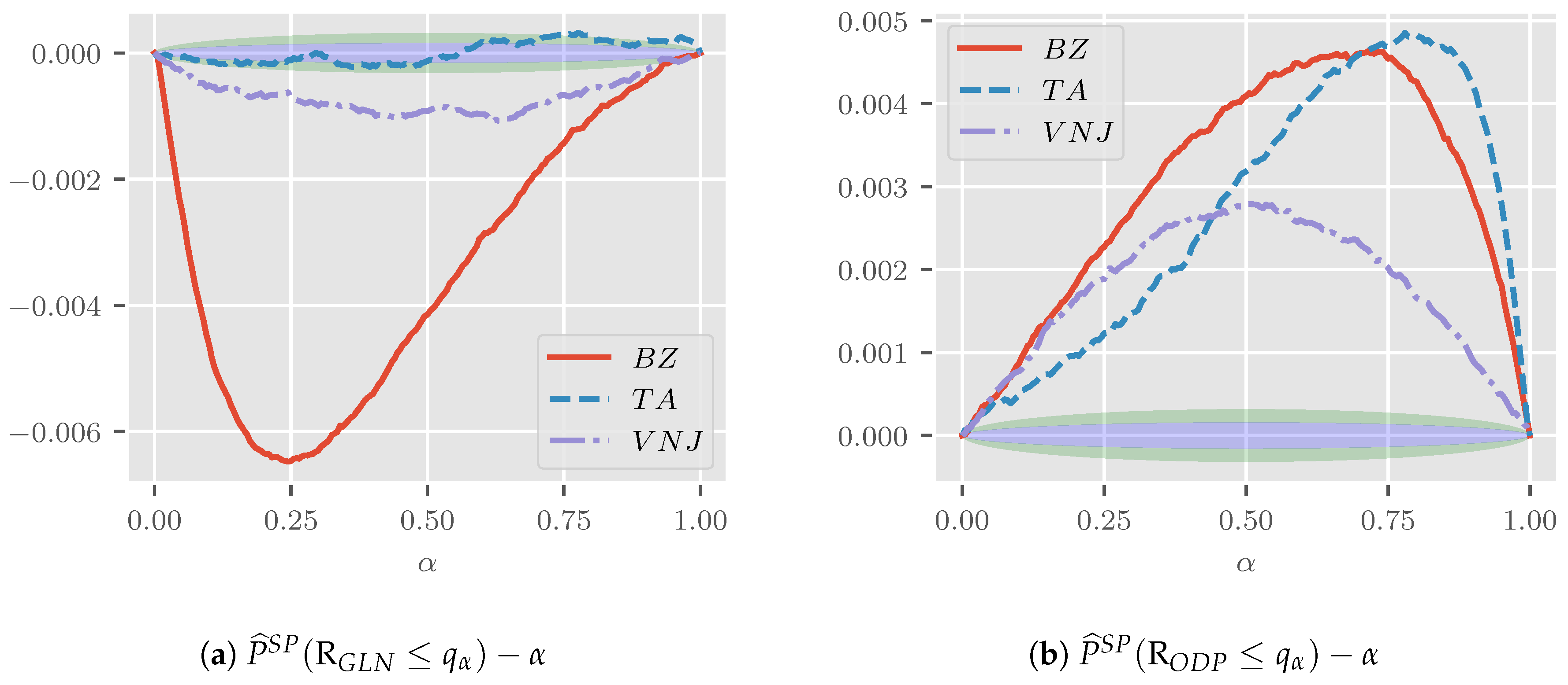
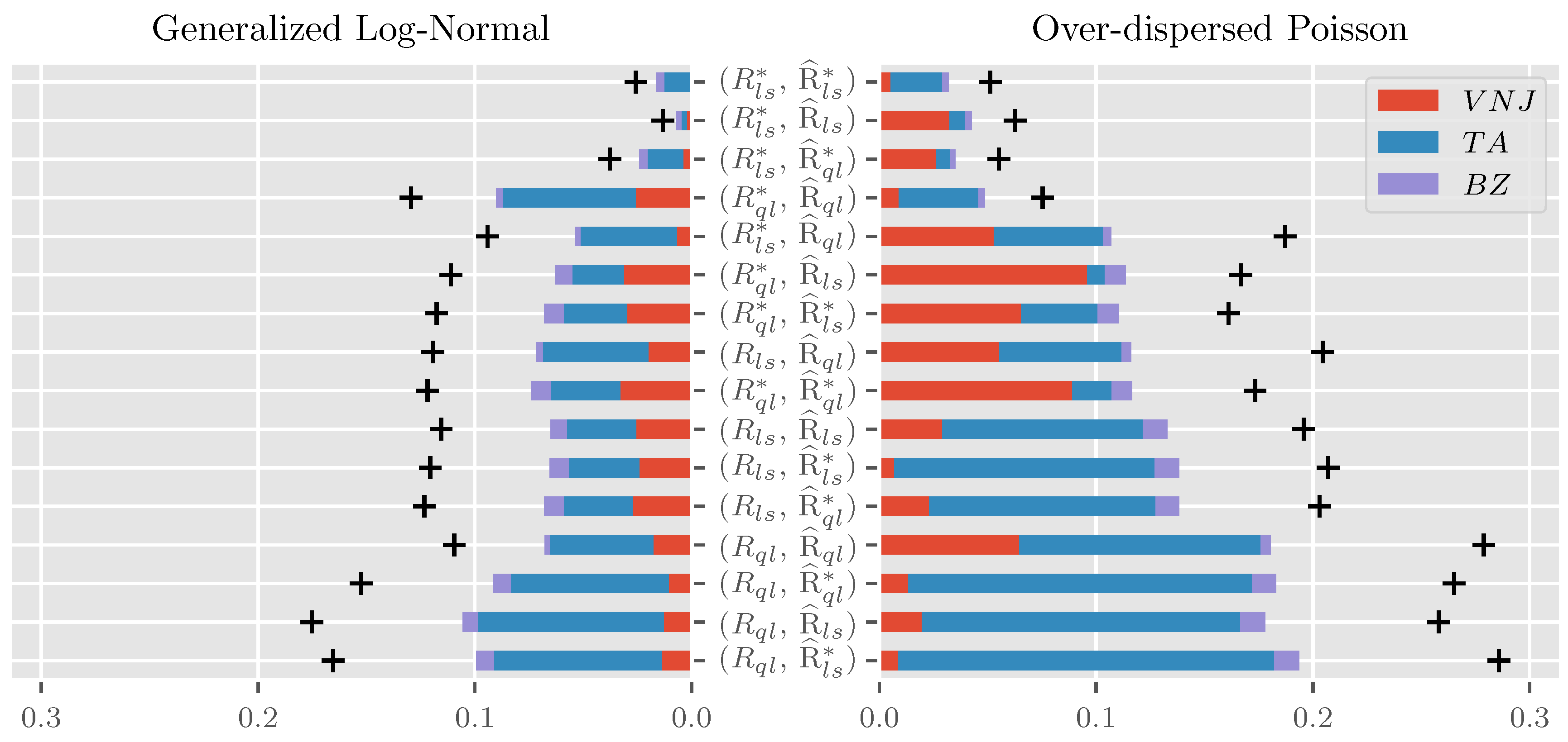
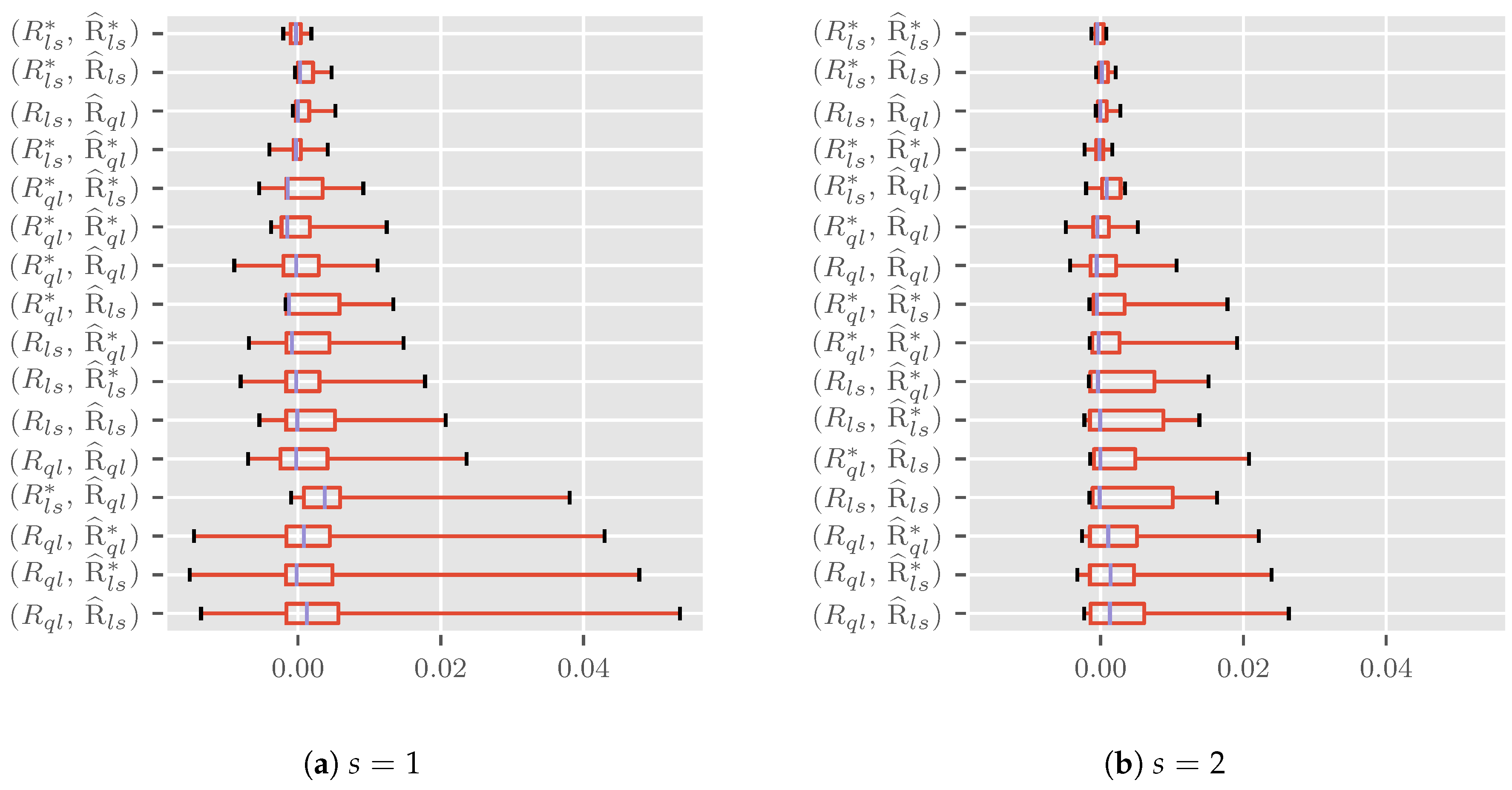
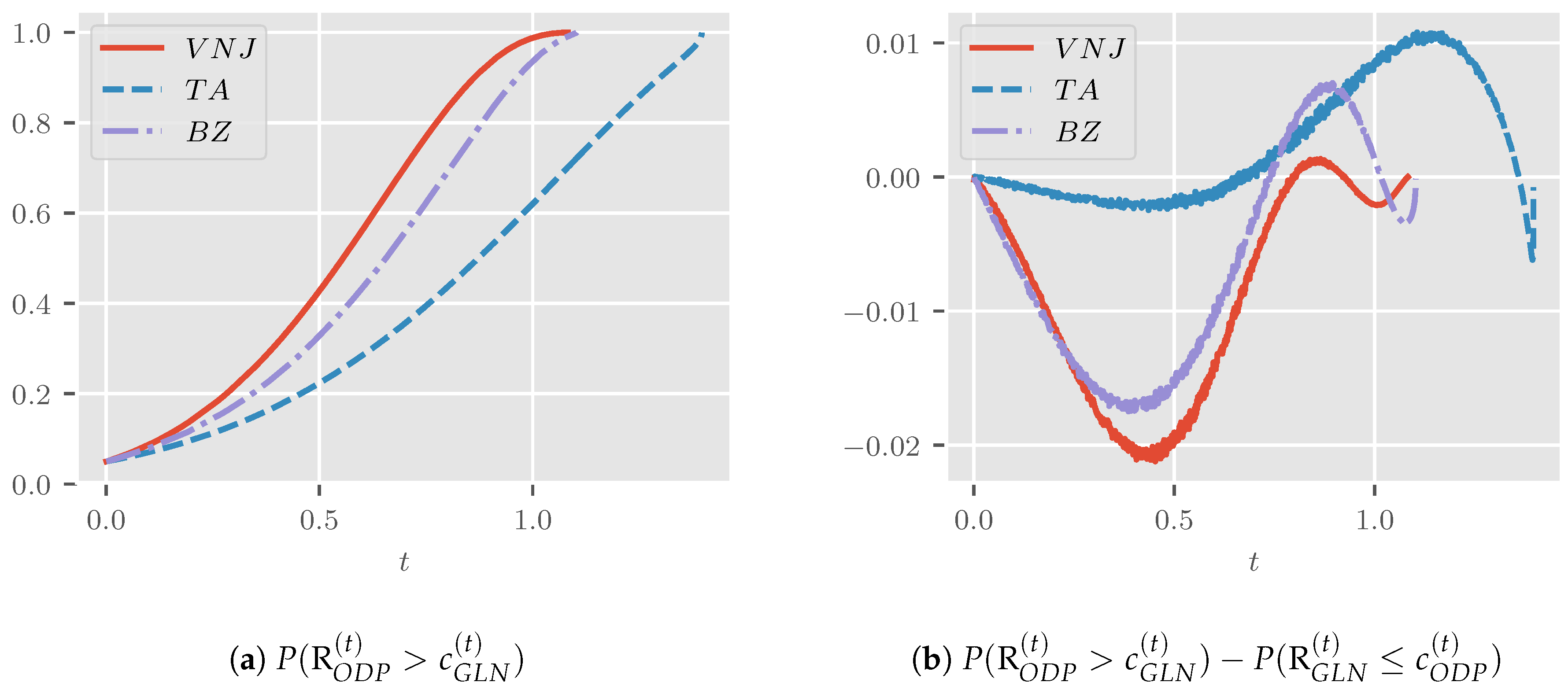
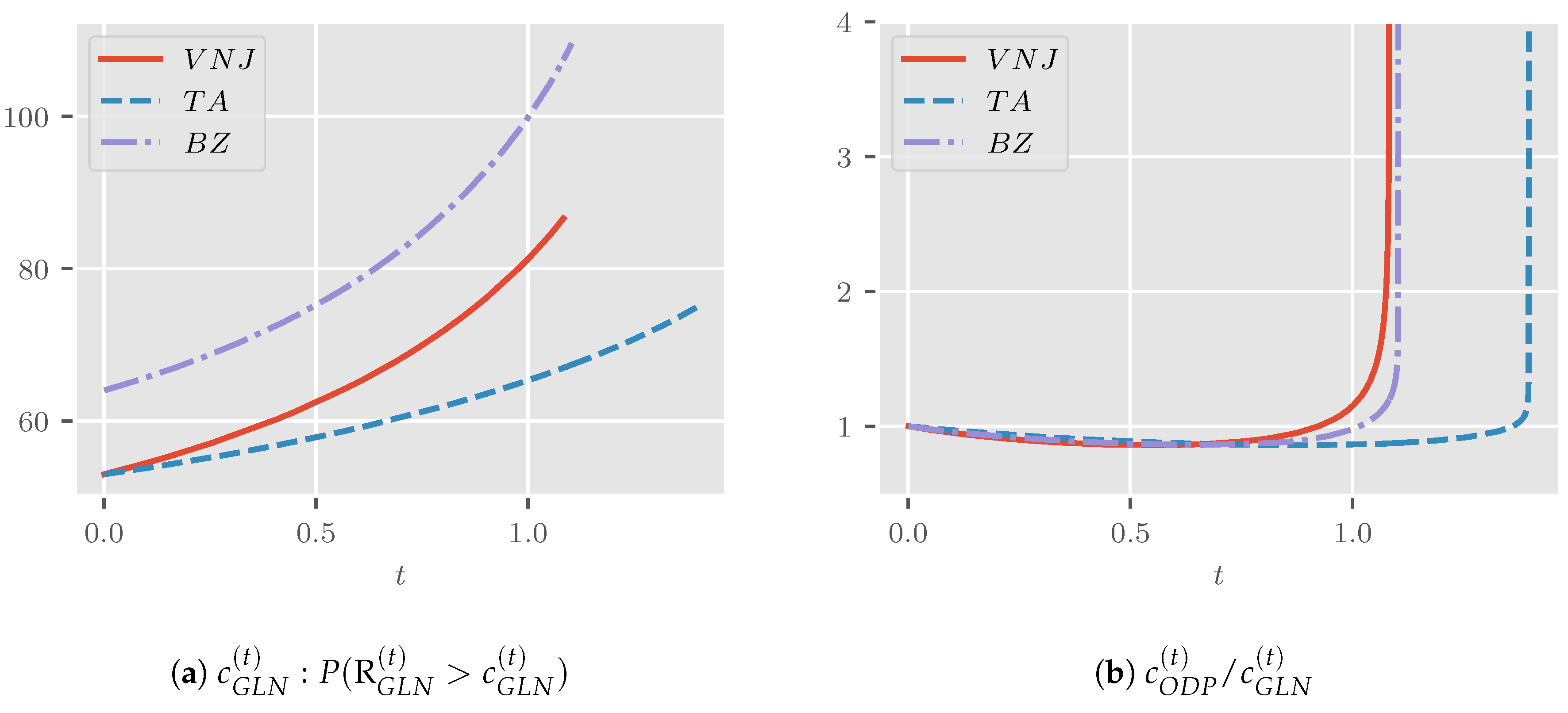
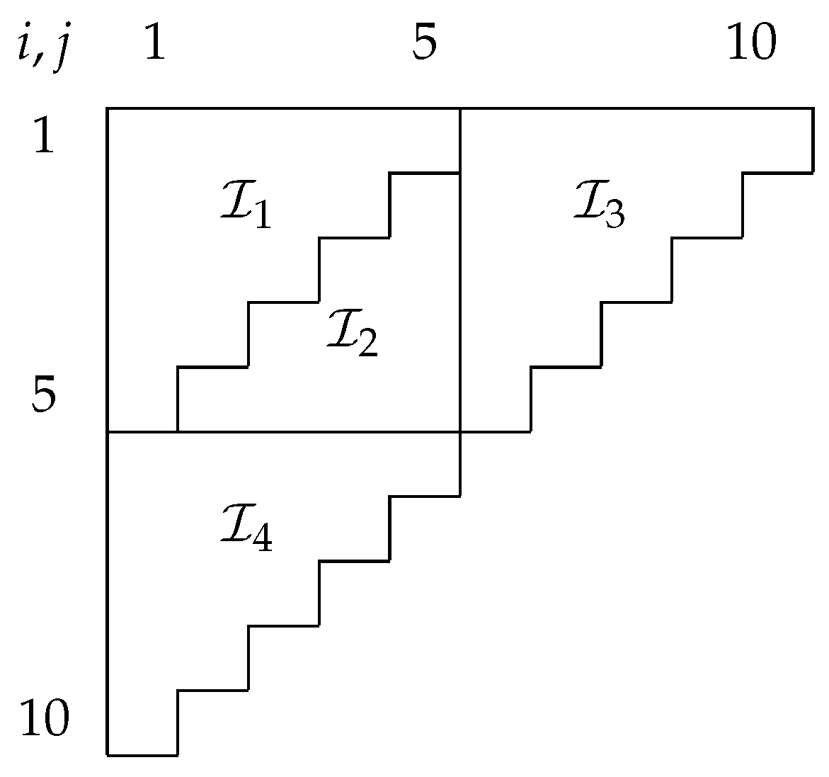
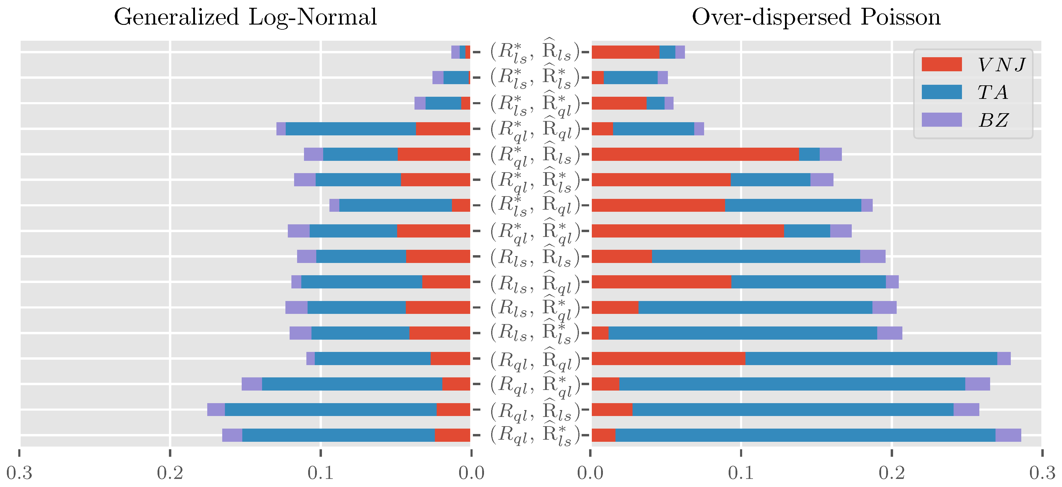
Table 1.
Run-off triangle taken from Verrall et al. (2010) with an indication for splitting into sub-samples corresponding to the first and last five accident years. Accident years i in the rows; development years j in the columns.
Table 1.
Run-off triangle taken from Verrall et al. (2010) with an indication for splitting into sub-samples corresponding to the first and last five accident years. Accident years i in the rows; development years j in the columns.
| 1 | 2 | 3 | 4 | 5 | 6 | 7 | 8 | 9 | 10 | |
|---|---|---|---|---|---|---|---|---|---|---|
| 01 | 451,288 | 339,519 | 333,371 | 144,988 | 093,243 | 045,511 | 25,217 | 20,406 | 31,482 | 1729 |
| 02 | 448,627 | 512,882 | 168,467 | 130,674 | 056,044 | 033,397 | 56,071 | 26,522 | 14,346 | - |
| 03 | 693,574 | 497,737 | 202,272 | 120,753 | 125,046 | 037,154 | 27,608 | 17,864 | - | - |
| 04 | 652,043 | 546,406 | 244,474 | 200,896 | 106,802 | 106,753 | 63,688 | - | - | - |
| 05 | 566,082 | 503,970 | 217,838 | 145,181 | 165,519 | 091,313 | - | - | - | - |
| 06 | 606,606 | 562,543 | 227,374 | 153,551 | 132,743 | - | - | - | - | - |
| 07 | 536,976 | 472,525 | 154,205 | 150,564 | - | - | - | - | - | - |
| 08 | 554,833 | 590,880 | 300,964 | - | - | - | - | - | - | - |
| 09 | 537,238 | 701,111 | - | - | - | - | - | - | - | - |
| 10 | 684,944 | - | - | - | - | - | - | - | - | - |
Table 2.
Power in % at critical values for large (over-dispersed Poisson DGP) and small (generalized log-normal DGP) along with the power gap in pp for the top four performers from Table 3. DGP is short for data generating process. Based on repetitions. .
Table 2.
Power in % at critical values for large (over-dispersed Poisson DGP) and small (generalized log-normal DGP) along with the power gap in pp for the top four performers from Table 3. DGP is short for data generating process. Based on repetitions. .
| DGP | |||||||
| 99.02 | 00.25 | 00.14 | 0.18 | 00.22 | |||
| 94.61 | −0.94 | −0.96 | −0.97 | −0.94 | |||
| 65.39 | 04.18 | 03.41 | 5.28 | 03.15 | |||
| - | |||||||
| 99.23 | −0.30 | −0.25 | −0.34 | −0.20 | |||
| 94.67 | −1.14 | −1.15 | −1.12 | −1.12 | |||
| 64.73 | 00.81 | 00.15 | 04.68 | 02.49 | |||
| : Generalized Log-Normal | : Over-Dispersed Poisson | |||||||
|---|---|---|---|---|---|---|---|---|
© 2018 by the author. Licensee MDPI, Basel, Switzerland. This article is an open access article distributed under the terms and conditions of the Creative Commons Attribution (CC BY) license (http://creativecommons.org/licenses/by/4.0/).
Share and Cite
MDPI and ACS Style
Harnau, J. Log-Normal or Over-Dispersed Poisson? Risks 2018, 6, 70. https://doi.org/10.3390/risks6030070
AMA Style
Harnau J. Log-Normal or Over-Dispersed Poisson? Risks. 2018; 6(3):70. https://doi.org/10.3390/risks6030070
Chicago/Turabian StyleHarnau, Jonas. 2018. "Log-Normal or Over-Dispersed Poisson?" Risks 6, no. 3: 70. https://doi.org/10.3390/risks6030070
APA StyleHarnau, J. (2018). Log-Normal or Over-Dispersed Poisson? Risks, 6(3), 70. https://doi.org/10.3390/risks6030070
Note that from the first issue of 2016, this journal uses article numbers instead of page numbers. See further details here.