Hierarchical Markov Model in Life Insurance and Social Benefit Schemes

Abstract

We explored the effect of the jump-diffusion process on a social benefit scheme consisting of life insurance, unemployment/disability benefits, and retirement benefits. To do so, we used a four-state Markov chain with multiple decrements. Assuming independent state-wise intensities taking the form of a jump-diffusion process and deterministic interest rates, we evaluated the prospective reserves for this scheme in which the individual is employed at inception. We then numerically demonstrated the state of the reserves for the scheme under jump-diffusion and non-jump-diffusion settings. By decomposing the reserve equation into five components, our numerical illustration indicated that an extension of the retirement age has a spillover effect that would increase government expenses for other social insurance programs. We also conducted sensitivity analyses and examined the total-reserves components by changing the relevant parameters of the transition intensities, which are the average jump-size parameter, average jump frequency, and diffusion parameters of the chosen states, with figures provided. Our computation revealed that the total reserve is most sensitive to changes in average jump frequency.

1. Introduction

While living longer healthily is a desirable life condition, longevity risks can affect a government’s ability to maintain fiscal sustenance and a balanced budget as a pension and social insurance scheme provider. Accompanied by lower birth rates, future employment would fall as the working population ages or becomes disabled, causing a nation to face lower productivity and higher age/unemployment/disability-related expenses.

Public pension schemes are used by governments to eliminate poverty among senior citizens, regardless of their working history, and sustain the standard of living previously enjoyed by retirees Willmore (2004). Governments have increasingly realized that the promises made under a pay-as-you-go social security system are hard to deliver; pension reforms have been conducted from as early as 1986 in the United States. While the exit rate from disability rolls in the United States has been trending upwards for the past decade (from 7.2% in 2004 to 9.3% in 2017), there is a chance that the population of beneficiaries would increase, particularly as female participation in the workforce increases (see Autor and Duggan 2006). Consequently, more workers may need to rely on government unemployment/disability benefits before they can access their pension funds if they involuntarily retire early as a result of a health condition. Because of increasing concern about the cost of supporting aging populations, governments all around the world have proposed changes to the retirement age (Duggan et al. (2005); Song and Manchester (2007)), which could delay pension annuity payments and potentially generate higher income tax revenue.

Over the period 1992–2008 in the United States, Chernew et al. (2016) found that healthy life expectancy at age 65 increased by 1.8 years, while disabled life expectancy fell by 0.5 years. This suggests that senior citizens are healthy enough to work longer and serves as an argument in favor of raising the retirement age. However, public economics research (see Gruber and Wise 2002 and Staubli and Zweim 2013) has shown evidence of weak employment opportunities for older workers resulting from the higher retirement age policy. Staubli and Zweim (2013) also found that while raising the early retirement age resulted in a net reduction of $229 million in the Austrian government’s expenditure, the reduced retirement benefit payments and higher tax revenues were counteracted by the spillover effects on the unemployment and disability insurance.

As summarized by Cairns et al. (2006) on the basis of the references within, mortality improvements are indeed stochastic. Additionally, modeling the morbidity and mortality rate as a jump-diffusion process seems viable given that chronic illness may occur as a shock event, thereby causing functional limitations as well as a disability (such as stroke-caused paralysis, heart attack, mental illness, or cancer). While some disabilities—such as musculoskeletal disease and mental disorder—are not terminal, the average duration of the disability can be quite long, thereby increasing the beneficiary population as well as the expected benefit amounts to be paid. The continuous affine processes used in Dahl (2004) and Biffis (2005) were applied to evaluate life insurance liabilities and disability annuities represented by a multistate Markov chain in Buchardt (2014) and Jang and Mohd Ramli (2015), respectively.

We ignore the possibility of individuals rejoining the employment pool after being made redundant as a result of either physical or mental disability, as we assume that losing physical functioning at a senior age would generally result in permanent impairment. Furthermore, a qualified benefit recipient is defined as an individual who has suffered from a medically determinable physical or mental impairment that is expected to result in death or last for at least a year and that prevents the person from engaging in a “substantial gainful activity” (Autor and Duggan 2006). The zero possibility of rejoining a state upon leaving is similar to studies by Buchardt (2014) and Olivieri and Ferri (2003), as opposed to studies conducted by Fong et al. (2015), who considered a Markov chain with transient states and an absorbing state.

This paper attempts to show the numerical effect of delaying retirement age, as it relates to the extra monetary burden shouldered by the policymakers should individuals react by taking the unemployment/disability benefits rather than working until the increased retirement age, leading to lower productivity. While the regression works on this issue can be noticed in Coe and Kelly (2010) and Atalay and Barrett (2015), our study extends the jump-diffusion framework in Jang and Mohd Ramli (2015) to represent the mortality, morbidity, redundancy, and retirement intensities of a four-state hierarchical Markov chain. The main contribution of this article is the numerical illustration of the model and the sensitivity analysis performed on the prospective reserve, which highlight the importance of selecting a model that captures the relevant features of such a scheme.

In Section 2, we present the results of a joint Laplace transform of the transition intensities following the jump-diffusion Cox–Ingersoll–Ross (CIR) process adopted from Jang and Mohd Ramli (2015). This is then followed by an analysis in Section 3 consisting of the life insurance and social benefit covers, entailing the probabilistic setup to describe the model framework. Section 4 shows how we applied the jump-diffusion model to the life insurance and social benefit scheme, using an example in which the state-wise intensities were independent. Assuming a deterministic rate of interest, we evaluated the prospective reserve for this scheme under the states Unemployed/Disabled, Retired, and Dead, where the employed were aged 45 in the Employed state at inception. We examined the sensitivity of prospective reserve components by changing the relevant parameters of the transition intensities, which are the jump size, average frequency of jumps, and diffusion parameters, and give their figure illustrations. Section 5 concludes the study.

2. Joint Laplace Transform of a Multivariate Jump-Diffusion CIR Model

In this section, we consider a jump-diffusion CIR process for the transition rates from state i, ${\lambda }_t^{(i)}$, which has the following structure:

$$d{\lambda }^{\left(i\right)}\left(t\right)=c^{\left(i\right)}\left(b^{\left(i\right)}+a^{\left(i\right)}{\lambda }^{\left(i\right)}\left(t\right)\right)dt+{\sigma }^{\left(i\right)}\sqrt{{\lambda }^{\left(i\right)}\left(t\right)}d{W}^{\left(i\right)}\left(t\right)+d{L}^{\left(i\right)}\left(t\right),$$

$$L^{\left(i\right)}\left(t\right)={\displaystyle \sum _{h=1}^{M^{(i)}\left(t\right)}}{Y}_h^{\left(i\right)},$$

(1)

where $c^{\left(i\right)}{b}^{\left(i\right)}$ represents the long-term mean level of the factor being modeled (state-wise transition intensity); $c^{\left(i\right)}{a}^{\left(i\right)}$ represents the drift coefficient, which is the speed at which the factor is driven back to its long-term mean with $c^{\left(i\right)}{a}^{\left(i\right)}<0$; ${\sigma }^{\left(i\right)}$ is the diffusion coefficient; and $W^{\left(i\right)}\left(t\right)$ is a standard Brownian motion governing the process. 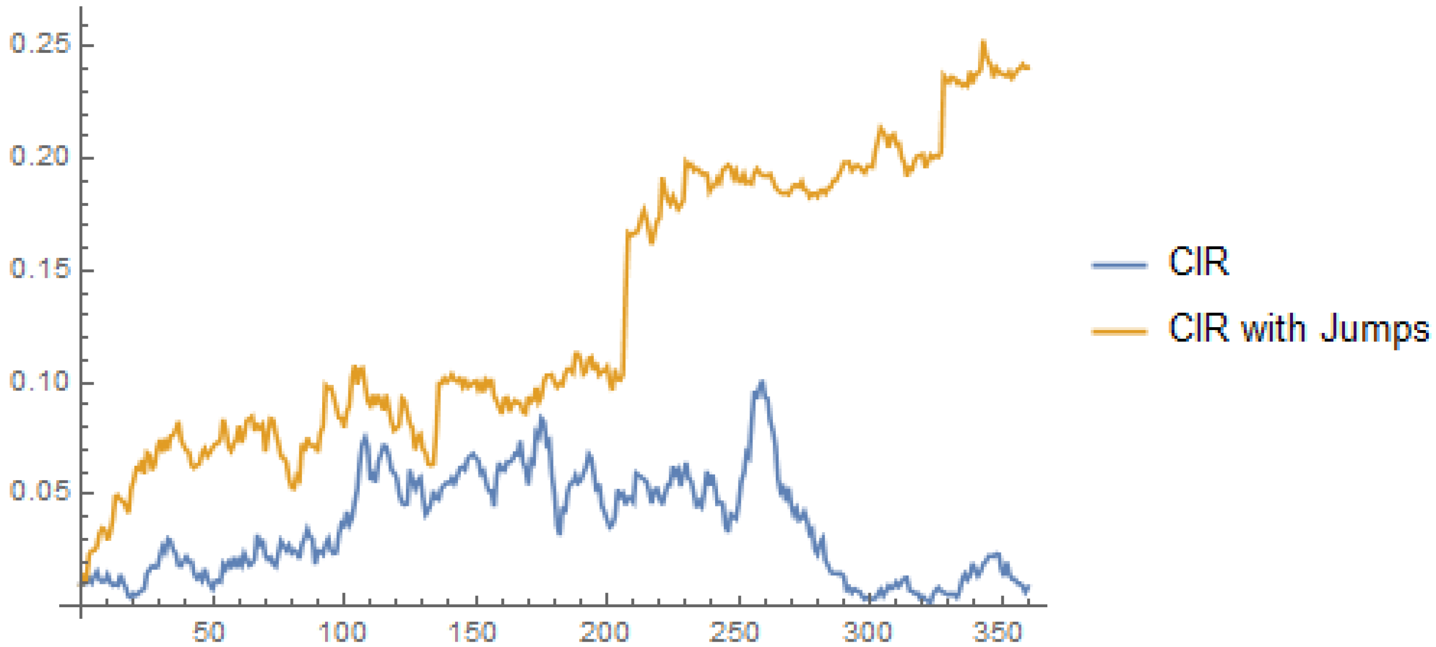Figure 1 illustrates simulated paths of the square-root process, one with jumps and the other without jumps.

We define $L^{\left(i\right)}\left(t\right)$ as a pure jump process in which $M^{(i)}(t)$ is the number of jumps, representing the total number of events up to time t and $Y_h,h=1,2,\cdots ,M^{(i)}(t)$ are their sizes. The point process $M^{(i)}(t)$ is independent of the vector sequence of jump sizes. The jump occurrences ${\rho }^{(i)}$ are assumed to be simultaneous for all states i and it is assumed that their sizes are independent and identically distributed (i.i.d.) with distribution function $F(y)$. The process needs to satisfy the usual Feller condition given by $\frac{2c^{(i)}{b}^{(i)}}{a^{(i)}}>{({\sigma }^{(i)})}^2$ to ensure ${\lambda }^{(i)}(t)>0$.

In this model, the dependence among intensities ${\lambda }^{(i)}(t)$ comes from the common event arrival process $M(t)$. We assume that the event arrival process $M^{(i)}(t)$ follows a homogeneous Poisson process with frequency parameter ${\rho }^{(i)}$ and that the jump size is exponentially distributed with average $\frac{1}{{\alpha }^{(i)}}$. A high value of ${\alpha }^{(i)}$ implies that on average, the magnitude of the jump sizes is small. Regardless of the jump-size distribution, we can impose dependency between the jump sizes of each intensity using a multivariate distribution such as a copula.

We also define the integrated transition intensities ${\mathsf{\Lambda }}^{(i)}\left(t\right)={\int }_0^t{\lambda }^{\left(i\right)}\left(s\right)ds$ for the purpose of derivation of the joint survival/non-unemployed (non-disabled)/non-retired probabilities in the next section. A low value of $c^{\left(i\right)}{a}^{\left(i\right)}$ implies that the process is reverting slowly to its long-term mean, since the parameter $c^{\left(i\right)}{a}^{\left(i\right)}$ represents the speed at which the intensity is being driven back to the long-term mean level, $c^{\left(i\right)}{b}^{\left(i\right)}$. Consequently, this will lead to higher values of ${\lambda }^{(i)}$ and ${\mathsf{\Lambda }}^{(i)}$, implying a higher chance of moving out of a particular state. Similarly, higher values of the initial intensity ${\lambda }_0^{(i)}$ and average jump frequency ${\rho }^{(i)}$ will lead to the same implication.

To arrive at the joint Laplace transform of the vector, $\left({\mathsf{\Lambda }}^{(1)}\left(t\right),\cdots ,{\mathsf{\Lambda }}^{(n)}\left(t\right)\right)$, we start by presenting the joint Laplace transform of the vector (${\mathsf{\Lambda }}^{(1)}(t),\cdots {\mathsf{\Lambda }}^{(n)}(t),{\lambda }^{(1)}(t),\cdots {\lambda }^{(n)}(t)$) at time t, conditional on the history of its evolution up to time t described by a filtration ${\mathcal{G}}_t=\sigma \left\{\left({\lambda }^{\left(1\right)}\left(s\right),\cdots ,{\lambda }^{\left(n\right)}\left(s\right)\right):s\le t\right\}$∈${\mathbb{R}}^n$ (see Corollary 2 in Jang and Mohd Ramli (2015)).

Proposition 1.

Considering constants ${\alpha }^{\left(i\right)}\ge 0$ and ${\gamma }^{\left(i\right)}\ge 0\forall i=1,\cdots ,n,$ the joint Laplace transform of the vector $\left({\mathsf{\Lambda }}^{(1)}\left(t\right),\cdots ,{\mathsf{\Lambda }}^{(n)}\left(t\right),{\lambda }^{\left(1\right)}\left(t\right),\cdots ,{\lambda }^{\left(n\right)}\left(t\right)\right)$ is given by

$$\begin{array}{c}\mathbb{E}\left[e^{-{\displaystyle \sum _{i=1}^n}{\gamma }^{(i)}{\mathsf{\Lambda }}^{(i)}\left(t\right)+{\alpha }^{\left(i\right)}{\lambda }^{(i)}\left(t\right)}|{\mathcal{G}}_0\right]\hfill \\ ={\displaystyle \prod _{i=1}^n}\left[H^{\left(i\right)}{\left(t\right)}^{\frac{2c^{(i)}{b}^{(i)}}{{\left({\sigma }^{(i)}\right)}^2}}\right]e^{-\left({\displaystyle \sum _{i=1}^n}{G}^{\left(i\right)}\left(t\right){\lambda }^{(i)}\left(0\right)+{\rho }^{(i)}{\int }_0^t\left[1-\widehat{c}\left(G^{\left(1\right)}\left(s\right),\cdots ,G^{\left(n\right)}\left(s\right)\right)\right]ds\right),}\hfill \end{array}$$

(2)

where $t>0$, with

$$G^{\left(i\right)}\left(t\right)=\frac{{\alpha }^{\left(i\right)}\left[\left(D^{\left(i\right)}+c^{(i)}{a}^{(i)}\right)+\left(D^{\left(i\right)}-c^{(i)}{a}^{(i)}\right)\exp \left\{-D^{\left(i\right)}t\right\}\right]+2{\gamma }^{(i)}\left(1-\exp \left\{-D^{\left(i\right)}t\right\}\right)}{{\left({\sigma }^{(i)}\right)}^2{\alpha }^{\left(i\right)}\left(1-\exp \left\{-D^{\left(i\right)}t\right\}\right)+\left(D^{\left(i\right)}-c^{(i)}{a}^{(i)}\right)+\left(D^{\left(i\right)}+c^{(i)}{a}^{(i)}\right)\exp \left\{-D^{\left(i\right)}t\right\}},$$

$$H^{\left(i\right)}\left(t\right)=\frac{2D^{\left(i\right)}\exp \left\{-\frac{D^{\left(i\right)}+c^{(i)}{a}^{(i)}}{2}t\right\}}{{\left({\sigma }^{(i)}\right)}^2{\alpha }^{\left(i\right)}\left(1-\exp \left\{D^{\left(i\right)}t\right\}\right)+\left(D^{\left(i\right)}-c^{(i)}{a}^{(i)}\right)+\left(D^{\left(i\right)}+c^{(i)}{a}^{(i)}\right)\exp \left\{D^{\left(i\right)}t\right\}},$$

$$\begin{array}{c}\widehat{c}\left({\zeta }^{\left(1\right)},\cdots ,{\zeta }^{\left(n\right)}\right)\hfill \\ ={\int }_0^{\infty }\stackrel{n}{\cdots }{\int }_0^{\infty }{e}^{-{\sum }_{i=1}^n{\zeta }^{\left(i\right)}{y}_i}\frac{{\partial }^{n}C\left(F_{Y^{\left(1\right)}}\left(y_1\right),\cdots ,F_{Y^{\left(n\right)}}\left(y_n\right)\right)}{\partial y_1\cdots \partial y_n}d{y}_1\cdots d{y}_n,\hfill \end{array}$$

and

$$D^{\left(i\right)}=\sqrt{{\left(c^{(i)}{a}^{(i)}\right)}^2+2{\left({\sigma }^{(i)}\right)}^2{\gamma }^{\left(i\right)}}.$$

We note that the joint Laplace transform contains a random element given by the term $\widehat{c}\left({\zeta }^{\left(1\right)},\cdots ,{\zeta }^{\left(n\right)}\right)$, which incorporates the jump-size distribution.

Proposition 2.

The joint Laplace transform of the vector $\left({\mathsf{\Lambda }}^{(1)}\left(t\right),\cdots ,{\mathsf{\Lambda }}^{(n)}\left(t\right)\right)$ is given by

$$\begin{array}{c}\mathbb{E}\left[\exp \left(-{\displaystyle \sum _{i=1}^n}{\gamma }^{(i)}{\mathsf{\Lambda }}^{\left(i\right)}\left(t\right)\right)|{\mathcal{G}}_0\right]\hfill \\ =\exp \left[-{\displaystyle \sum _{i=1}^n}{G}^{(i)}\left(t\right){\lambda }^{\left(i\right)}\left(0\right)\right]\times {\displaystyle \prod _{i=1}^n}\left[H^{\left(i\right)}{\left(t\right)}^{\frac{2c^{(i)}{b}^{(i)}}{{\left({\sigma }^{(i)}\right)}^2}}\right]\hfill \\ \times \exp \left[-\rho {\int }_0^t\left[1-\widehat{c}\left(G^{\left(1\right)}\left(s\right),\cdots ,G^{\left(n\right)}\left(s\right)\right)ds\right]\right].\hfill \end{array}$$

(3)

Equation (3) is used to compute the survival/non-unemployed (non-disabled)/non-retired probabilities, which are needed in order to evaluate the prospective reserve of the life insurance and social benefit scheme in Section 4.

3. Multiple State Model for Life Insurance and Social Benefit Covers

We adopt a setup similar to Jang and Mohd Ramli (2015) whereby we focus on an employed individual aged x at time 0. We work under a filtered probability space $\left(\Omega ,\mathcal{F},\mathbb{F},\mathbb{P}\right)$, consisting of the sample space $\Omega ,$ the $\sigma$-algebra $\mathcal{F}$, the probability measure $\mathbb{P}$, and a filtration $\mathbb{F}={\left({\mathcal{F}}_t\right)}_{t\ge 0}$, which satisfy the usual completeness and right continuity conditions, as in Protter (1990). The filtration $\mathbb{F}$ represents the information available up to time t. We consider the setup in which $\mathbf{Z}={(Z(t))}_{t\in {\mathbb{R}}_{+}}$ is a Markov process governed by the transition rates ${\left({\lambda }_x^{\left(ij\right)}\left(t\right)\right)}_{t\in \mathbb{R}}$ in the finite state space $\mathcal{J}$, representing the state of the employed individual: employed, unemployed/disabled, retired, or dead. The employed individual’s random residual lifetime is modeled as an $\mathbb{F}$-stopping time ${\tau }_x^{\left(ij\right)}$, admitting a random intensity ${\lambda }_x^{\left(ij\right)}$ (i.e., ${\tau }_x^{\left(ij\right)}\equiv \inf \left\{t:N^{\left(ij\right)}\left(t\right)=1|N^{\left(ij\right)}\left(0\right)=0\right\}$). Intuitively, ${\tau }_x^{\left(ij\right)}$ denotes the first jump time of a nonexplosive $\mathbb{F}$-counting process $N^{\left(ij\right)}\left(t\right)$ recording at each time $t\ge 0$ whether the employed individual has died, has become unemployed or disabled, has retired $\left(N^{\left(ij\right)}\left(t\right)\ne 0\right)$, or is still employed $\left(N^{\left(ij\right)}\left(t\right)=0\right)$. The counting process $N^{\left(ij\right)}\left(t\right)$ is a Cox process driven by sub-filtration $\mathbb{G}$ of $\mathbb{F}$, with $\mathbb{G}$-predictable intensity ${\lambda }_x^{\left(ij\right)}$.

We also assume that ${\lambda }_x^{\left(ij\right)}\ge 0$ is a predictable process such that ${\int }_0^t{\lambda }_x^{\left(ij\right)}\left(s\right)ds\le \infty$ for all $t\ge 0$ and that the compensated process $\mathcal{S}=\left\{N^{\left(ij\right)}\left(t\right)-{\int }_0^t{\lambda }_x^{\left(ij\right)}\left(s\right)ds:t\ge 0\right\}$ is a local $\mathbb{F}$-martingale. Additionally, if $\mathbb{E}\left[{\int }_0^t{\lambda }_x^{\left(ij\right)}\left(s\right)ds\right]<\infty$ for all $t\ge 0$, then $\mathcal{S}$ is an $\mathbb{F}$-martingale. In other words, $N^{\left(ij\right)}\left(t\right)$ follows an inhomogeneous Poisson process with parameter ${\int }_0^t{\lambda }^{\left(ij\right)}\left(s\right)ds$. The information provided by the sub-filtration $\mathbb{G}$ is sufficient to suggest the likelihood of an event happening but is not enough to indicate if it has actually occurred.

We can then define the instantaneous event probability at any time $t\ge 0$, in state $\omega \in \Omega$ such that ${\tau }_x^{\left(ij\right)}>t$ , and for small $dt>0$ as

$$\mathbb{P}\left({\tau }_x^{\left(ij\right)}\le t+dt|{\mathcal{F}}_t\right)\left(\omega \right)\cong {\lambda }_x^{\left(ij\right)}\left(t,\omega \right)dt.$$

(4)

The value given by Equation (4) varies as the information related to the employed individual’s social and health status unfolds. Furthermore, assuming that the employed individual is representative of a group of retirement fund contributors and that the random residual lifetimes are an i.i.d. variable, we drop the reference to the age x from now on and set ${\tau }^{\left(ij\right)}={\tau }_x^{\left(ij\right)}$ and ${\lambda }^{\left(ij\right)}\left(t\right)={\lambda }_x^{\left(ij\right)}\left(t\right)$.

The transition rates are modeled as a d-dimensional jump-diffusion process as in Section 2. As the filtration $\mathbb{F}={\left({\mathcal{F}}_t\right)}_{t\ge 0}$ reveals the knowledge of the evolution of all state variables up to time t (information revealed by $\mathbf{Z}$) and of whether the employed has changed state by then (information revealed by ${\mathcal{G}}_t$), we then write ${\mathcal{F}}_t={\mathcal{G}}_t\vee {\mathcal{H}}_t$, where ${\mathcal{G}}_t\vee {\mathcal{H}}_t$ is the $\sigma$-algebra generated by ${\mathcal{G}}_t\cup {\mathcal{H}}_t$, with

$$\begin{array}{ccc}\hfill {\mathcal{G}}_t& =& \sigma \left({\lambda }^{\left(ij\right)}\left(s\right):0\le s\le t\forall i,j\right),\hfill \\ \hfill {\mathcal{H}}_t& =& \sigma \left({\mathbb{I}}_{\left\{\tau \le s\right\}}:0\le s\le t\right).\hfill \end{array}$$

Therefore, the filtration $\mathbb{F}=\mathbb{G}\vee \mathbb{H},$ with $\mathbb{H}={\left({\mathcal{H}}_t\right)}_{t\ge 0}$ being the smallest filtration revealing information on the stopping time ${\tau }^{\left(ij\right)}$.

We consider a life insurance and social benefit scheme with accumulated payments until time t given by the following dynamics:

$$dB\left(t\right)={\displaystyle \sum _{i\in \mathcal{J}}}{1}_{\left\{Z(t)=i\right\}}^{\left(i\right)}{\kappa }^{\left(i\right)}\left(t\right)+{\displaystyle \sum _{\begin{array}{c}i,j\in \mathcal{J}\\ i\ne j\end{array}}}{\kappa }^{\left(ij\right)}\left(t\right)d{N}^{\left(ij\right)}\left(t\right),$$

where ${\kappa }^{\left(i\right)}\left(t\right)$ is the payment while the employed individual is in state i at time t and ${\kappa }^{\left(ij\right)}\left(t\right)$ represents the payment paid to the employed individual upon jumping from state i to j at time t. For the purpose of reserve computation, we evaluate the prospective reserve of the benefits given by

$$V\left(t\right)=E\left[{\int }_t^{\infty }{e}^{-{\int }_t^{s}r\left(\tau \right)d\tau }dB\left(s\right)|{\mathcal{F}}_t\right],$$

which is the expected present value of the future payments conditional on the information available at time t. One can consider taking the expectation under the risk-neutral, pricing, or market measures.

4. Numerical Example

We consider an individual aged 45 at inception and assume that individuals who were made redundant or who become disabled will not be able to rejoin the employment pool. Given a finite state space $\mathcal{J}$, we associate a set of non-negative transition rates ${\lambda }^{\left(jk\right)}\left(t\right)$ with $j,k\in$$\mathcal{J}$ such that it is a hierarchical Markov chain. We refer the readers to Haberman and Pitacco (1999) for a more extensive description of this model in the insurance context. Similarly to Buchardt (2014) and Jang and Mohd Ramli (2015), we apply the jump-diffusion CIR process to model the transition rates for the four-state Markov chain with the framework as defined in the previous section. 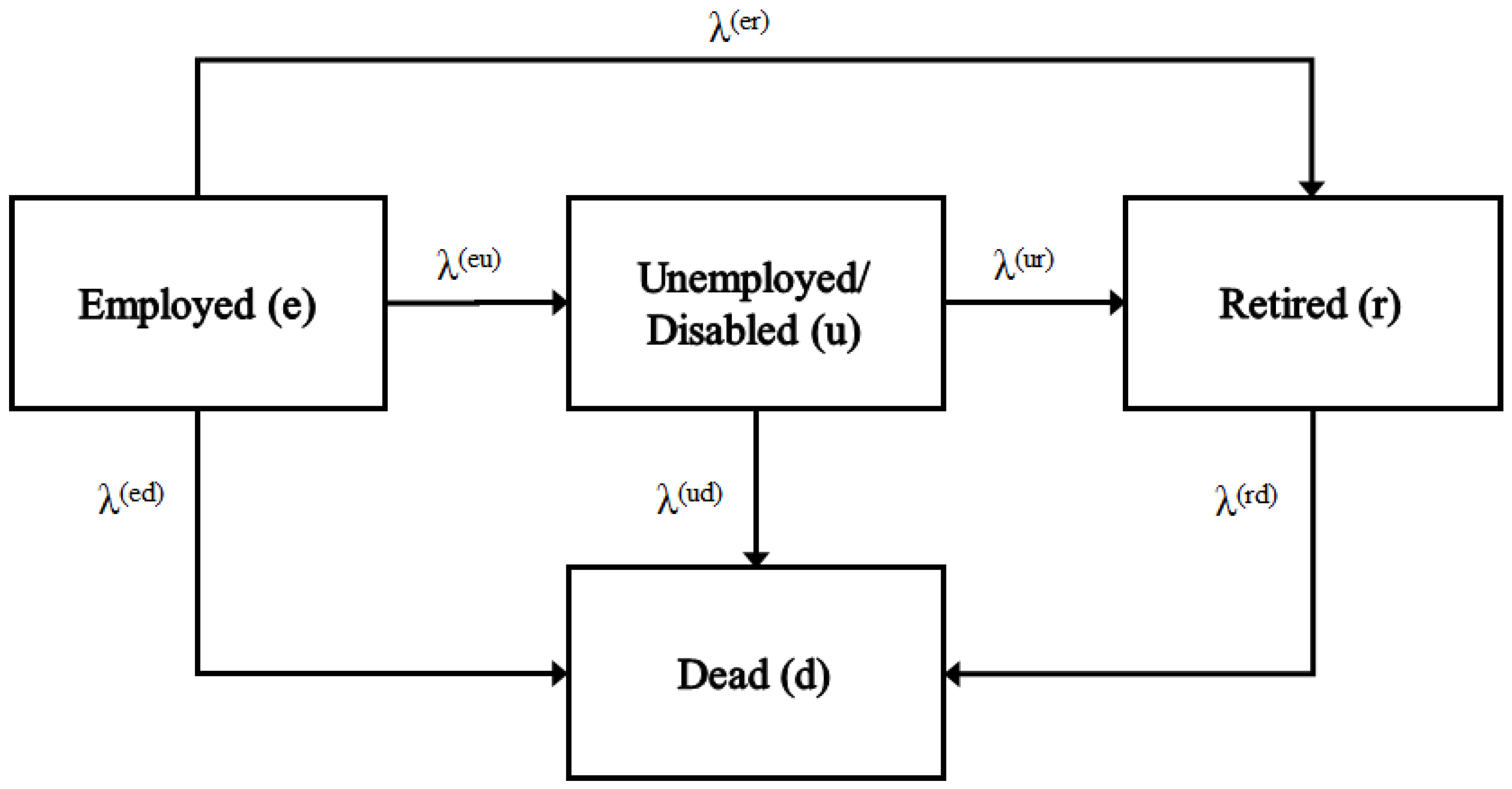We consider a model with four states, $\mathcal{J}=\left\{e,u/i,r,d\right\},$ corresponding to Employed, Unemployed/Disabled (i.e., permanent redundancy/disability), Retired, and Dead, respectively, as depicted in Figure 2. The scenarios of redundancy and disability are pooled in the same state. This is a four-state model with three causes of decrement, two causes of second-order decrement, and a third-order decrement.

We let $T_1$ denote the retirement age after which the employed individual is entitled to have their occupational pension invested or accumulated while they continue to work. Given that $T_2$ is the maximum survival age, no payment is made after $T_2$. Additionally, should death occur before time $T_1$ or between $T_1$ and $T_2$, the employed individual will receive accumulated contributions as a (lump-sum) death benefit. The scheme under this model stipulates that the employed individual will be paid the continuous payment ${\kappa }^{\left(u\right)}\left(t\right)$ or ${\kappa }^{\left(r\right)}\left(t\right)$ while in the Unemployed/Disabled or Retired state and that an amount ${\kappa }^{\left(ed\right)}\left(t\right)$, ${\kappa }^{\left(ud\right)}\left(t\right)$, or ${\kappa }^{\left(rd\right)}\left(t\right)$ is payable should death occur at time t from the Employed, Unemployed/Disabled, or Retired state, respectively. The total payment for the benefits considered under this model is given by the process $B\left(t\right)$, satisfying the following:

$$\begin{array}{ccc}\hfill dB\left(t\right)& =& {\kappa }^{\left(ed\right)}\left(t\right)d{N}^{\left(ed\right)}\left(t\right)+{\kappa }^{\left(u\right)}\left(t\right){\mathbf{1}}_{\left(Z\left(t\right)=u\right)}dt+{\kappa }^{\left(ud\right)}\left(t\right)d{N}^{\left(ud\right)}\left(t\right)\hfill \\ & & +{\kappa }^{\left(r\right)}\left(t\right){\mathbf{1}}_{\left(Z\left(t\right)=r\right)}dt+{\kappa }^{\left(rd\right)}\left(t\right)d{N}^{\left(rd\right)}\left(t\right).\hfill \end{array}$$

To assess the impact of the increase in retirement age on government expenditures, we now assume that ${\kappa }^{\left(u\right)}\left(t\right)$ and ${\kappa }^{\left(r\right)}\left(t\right)$ are paid by a government social welfare system (i.e., unemployment/disabled benefits and age pension benefits, denoted henceforth as ${\kappa }_G^{\left(u\right)}(t)$ and ${\kappa }_G^{\left(r\right)}(t)$, respectively). Assuming that the payments are deterministic and that there are no payments after time $T_2$, the prospective reserve equation can be expanded as follows:

$$\begin{array}{c}{\kappa }^{\left(ed\right)}{\int }_{t_1}^{T_1}\left\{e^{-{\int }_{t_1}^s\left(r_{\tau }+{\lambda }^{\left(ed\right)}\left(\tau \right)+{\lambda }^{\left(eu\right)}\left(\tau \right)+{\lambda }^{\left(er\right)}\left(\tau \right)\right)d\tau }{\lambda }^{\left(ed\right)}\left(s\right)\right\}ds\hfill \\ +{\int }_{t_1}^{T_1}\left\{\begin{array}{c}{e}^{-{\int }_{t_1}^s\left(r_{\tau }+{\lambda }^{\left(ed\right)}\left(\tau \right)+{\lambda }^{\left(eu\right)}\left(\tau \right)+{\lambda }^{\left(er\right)}\left(\tau \right)\right)d\tau }{\lambda }^{\left(eu\right)}\left(s\right)\\ \times \left[{\int }_s^{T_1}{e}^{-{\int }_s^u\left(r_{\tau }+{\lambda }^{\left(ur\right)}\left(\tau \right)+{\lambda }^{\left(ud\right)}\left(\tau \right)\right)d\tau }\left({\kappa }_G^{\left(u\right)}+{\kappa }^{\left(ud\right)}{\lambda }^{\left(ud\right)}\left(u\right)\right)du\right]\end{array}\right\}ds\hfill \\ +{\int }_{t_1}^{T_1}\left\{\begin{array}{c}{e}^{-{\int }_{t_1}^s\left(r_{\tau }+{\lambda }^{\left(ed\right)}\left(\tau \right)+{\lambda }^{\left(eu\right)}\left(\tau \right)+{\lambda }^{\left(er\right)}\left(\tau \right)\right)d\tau }{\lambda }^{\left(eu\right)}\left(s\right)\\ \times \left[\begin{array}{c}{\int }_s^{T_1}{e}^{-{\int }_s^u\left(r_{\tau }+{\lambda }^{\left(ur\right)}\left(\tau \right)+{\lambda }^{\left(ud\right)}\left(\tau \right)\right)d\tau }\\ \times \left[{\int }_{T_1}^{T_2}{e}^{-{\int }_{T_1}^{\nu }\left(r_{\tau }+{\lambda }^{\left(rd\right)}\left(\tau \right)\right)d\tau }\left({\kappa }_G^{\left(r\right)}+{\kappa }^{\left(rd\right)}{\lambda }^{\left(rd\right)}\left(\nu \right)\right)d\nu \right]\end{array}\right]du\end{array}\right\}ds.\hfill \end{array}$$

(5)

Using the multivariate jump-diffusion process in Section 2 as the transition intensities, the survival/non-unemployed (non-disabled)/non-retired probability expression is relatively simple to obtain. However, the term $\mathbb{E}\left[e^{-{\int }_{t_1}^s{\lambda }^{\left(er\right)}\left(\tau \right)d\tau }|{\mathcal{F}}_{t_1}\right]$ for the case of dependent transition rate is yet to be derived, as mentioned in Buchardt (2014) and Jang and Mohd Ramli (2015). Had the explicit form of the term been obtained, one could examine the effect of applying various dependence structures among the transition intensities using a multivariate distribution or a copula, which we leave for further research.

For simplicity, we use the deterministic short rate, r, instead of the stochastic financial environment. Then, taking expectation of Equation (5) and assuming independence between the six transition rates ${\lambda }^{\left(ed\right)}\left(s\right)$, ${\lambda }^{\left(eu\right)}\left(s\right),$ ${\lambda }^{\left(er\right)}\left(s\right)$, ${\lambda }^{\left(ud\right)}\left(s\right)$, ${\lambda }^{\left(ur\right)}\left(s\right)$, and ${\lambda }^{\left(rd\right)}\left(s\right)$, we obtain the following:

$$\begin{array}{c}{\kappa }^{\left(ed\right)}{\int }_{t_1}^{T_1}{e}^{-r\left(s-t_1\right)}\mathbb{E}\left[e^{-{\int }_{t_1}^s{\lambda }^{\left(ed\right)}\left(\tau \right)d\tau }{\lambda }^{\left(ed\right)}\left(s\right)|{\mathcal{F}}_{t_1}\right]\mathbb{E}\left[e^{-{\int }_{t_1}^s{\lambda }^{\left(eu\right)}\left(\tau \right)d\tau }|{\mathcal{F}}_{t_1}\right]\hfill \\ \times \mathbb{E}\left[e^{-{\int }_{t_1}^s{\lambda }^{\left(er\right)}\left(\tau \right)d\tau }|{\mathcal{F}}_{t_1}\right]ds\hfill \\ +{\kappa }_G^{\left(u\right)}{\int }_{t_1}^{T_1}{\int }_s^{T_1}{e}^{-r\left(u-t_1\right)}\mathbb{E}\left[e^{-{\int }_{t_1}^s{\lambda }^{\left(ed\right)}\left(\tau \right)d\tau }|{\mathcal{F}}_{t_1}\right]\mathbb{E}\left[e^{-{\int }_{t_1}^s{\lambda }^{\left(eu\right)}\left(\tau \right)d\tau }{\lambda }^{\left(eu\right)}\left(s\right)|{\mathcal{F}}_{t_1}\right]\hfill \\ \times \mathbb{E}\left[e^{-{\int }_{t_1}^s{\lambda }^{\left(er\right)}\left(\tau \right)d\tau }|{\mathcal{F}}_{t_1}\right]\mathbb{E}\left[e^{-{\int }_s^u{\lambda }^{\left(ur\right)}\left(\tau \right)d\tau }|{\mathcal{F}}_{t_1}\right]\mathbb{E}\left[e^{-{\int }_s^u{\lambda }^{\left(ud\right)}\left(\tau \right)d\tau }|{\mathcal{F}}_{t_1}\right]duds\hfill \\ +{\kappa }^{\left(ud\right)}{\int }_{t_1}^{T_1}{\int }_s^{T_1}{e}^{-r\left(u-t_1\right)}\mathbb{E}\left[e^{-{\int }_{t_1}^s{\lambda }^{\left(ed\right)}\left(\tau \right)d\tau }|{\mathcal{F}}_{t_1}\right]\mathbb{E}\left[e^{-{\int }_{t_1}^s{\lambda }^{\left(eu\right)}\left(\tau \right)d\tau }{\lambda }^{\left(eu\right)}\left(s\right)|{\mathcal{F}}_{t_1}\right]\hfill \\ \times \mathbb{E}\left[e^{-{\int }_{t_1}^s{\lambda }^{\left(er\right)}\left(\tau \right)d\tau }|{\mathcal{F}}_{t_1}\right]\mathbb{E}\left[e^{-{\int }_s^u{\lambda }^{\left(ur\right)}\left(\tau \right)d\tau }|{\mathcal{F}}_{t_1}\right]\mathbb{E}\left[e^{-{\int }_s^u{\lambda }^{\left(ud\right)}\left(\tau \right)d\tau }{\lambda }^{\left(ud\right)}\left(u\right)|{\mathcal{F}}_{t_1}\right]duds\hfill \\ +{\kappa }_G^{\left(r\right)}{\int }_{t_1}^{T_1}{\int }_s^{T_1}{\int }_{T_1}^{T_2}{e}^{-r\left(u-t_1\right)}{e}^{-r\left(\nu -T_1\right)}\mathbb{E}\left[e^{-{\int }_{t_1}^s{\lambda }^{\left(ed\right)}\left(\tau \right)d\tau }|{\mathcal{F}}_{t_1}\right]\hfill \\ \times \mathbb{E}\left[e^{-{\int }_{t_1}^s{\lambda }^{\left(eu\right)}\left(\tau \right)d\tau }{\lambda }^{\left(eu\right)}\left(s\right)|{\mathcal{F}}_{t_1}\right]\mathbb{E}\left[e^{-{\int }_{t_1}^s{\lambda }^{\left(er\right)}\left(\tau \right)d\tau }|{\mathcal{F}}_{t_1}\right]\hfill \\ \times \mathbb{E}\left[e^{-{\int }_s^u{\lambda }^{\left(ur\right)}\left(\tau \right)d\tau }|{\mathcal{F}}_{t_1}\right]\mathbb{E}\left[e^{-{\int }_s^u{\lambda }^{\left(ud\right)}\left(\tau \right)d\tau }|{\mathcal{F}}_{t_1}\right]\mathbb{E}\left[e^{-{\int }_{T_1}^{\nu }{\lambda }^{\left(rd\right)}\left(\tau \right)d\tau }|{\mathcal{F}}_{t_1}\right]d\nu duds\hfill \\ +{\kappa }^{\left(rd\right)}{\int }_{t_1}^{T_1}{\int }_s^{T_1}{\int }_{T_1}^{T_2}{e}^{-\delta \left(u-t_1\right)}{e}^{-\delta \left(\nu -T_1\right)}\mathbb{E}\left[e^{-{\int }_{t_1}^s{\lambda }^{\left(ed\right)}\left(\tau \right)d\tau }|{\mathcal{F}}_{t_1}\right]\hfill \\ \times \mathbb{E}\left[e^{-{\int }_{t_1}^s{\lambda }^{\left(eu\right)}\left(\tau \right)d\tau }{\lambda }^{\left(eu\right)}\left(s\right)|{\mathcal{F}}_{t_1}\right]\mathbb{E}\left[e^{-{\int }_{t_1}^s{\lambda }^{\left(er\right)}\left(\tau \right)d\tau }|{\mathcal{F}}_{t_1}\right]\hfill \\ \times \mathbb{E}\left[e^{-{\int }_s^u{\lambda }^{\left(ur\right)}\left(\tau \right)d\tau }|{\mathcal{F}}_{t_1}\right]\mathbb{E}\left[e^{-{\int }_s^u{\lambda }^{\left(ud\right)}\left(\tau \right)d\tau }|{\mathcal{F}}_{t_1}\right]\hfill \\ \mathbb{E}\left[e^{-{\int }_{T_1}^{\nu }{\lambda }^{\left(rd\right)}\left(\tau \right)d\tau }{\lambda }^{\left(rd\right)}\left(\nu \right)|{\mathcal{F}}_{t_1}\right]d\nu duds.\hfill \end{array}$$

(6)

We examine the five components of Equation (6). Component 1,

$$\begin{array}{c}{\kappa }^{\left(ed\right)}{\int }_{t_1}^{T_1}{e}^{-r\left(s-t_1\right)}\mathbb{E}\left[e^{-{\int }_{t_1}^s{\lambda }^{\left(ed\right)}\left(\tau \right)d\tau }{\lambda }^{\left(ed\right)}\left(s\right)|{\mathcal{F}}_{t_1}\right]\mathbb{E}\left[e^{-{\int }_{t_1}^s{\lambda }^{\left(eu\right)}\left(\tau \right)d\tau }|{\mathcal{F}}_{t_1}\right]\hfill \\ \times \mathbb{E}\left[e^{-{\int }_{t_1}^s{\lambda }^{\left(er\right)}\left(\tau \right)d\tau }|{\mathcal{F}}_{t_1}\right]ds,\hfill \end{array}$$

represents the immediate lump-sum payment made to the beneficiary upon the death of the individual while in the Employed state. Analogously, component 2,

$$\begin{array}{c}{\kappa }_G^{\left(u\right)}{\int }_{t_1}^{T_1}{\int }_s^{T_1}{e}^{-r\left(u-t_1\right)}\mathbb{E}\left[e^{-{\int }_{t_1}^s{\lambda }^{\left(ed\right)}\left(\tau \right)d\tau }|{\mathcal{F}}_{t_1}\right]\mathbb{E}\left[e^{-{\int }_{t_1}^s{\lambda }^{\left(er\right)}\left(\tau \right)d\tau }|{\mathcal{F}}_{t_1}\right]\hfill \\ \times \mathbb{E}\left[e^{-{\int }_{t_1}^s{\lambda }^{\left(eu\right)}\left(\tau \right)d\tau }{\lambda }^{\left(eu\right)}\left(s\right)|{\mathcal{F}}_{t_1}\right]\mathbb{E}\left[e^{-{\int }_s^u{\lambda }^{\left(ur\right)}\left(\tau \right)d\tau }|{\mathcal{F}}_{t_1}\right]\mathbb{E}\left[e^{-{\int }_s^u{\lambda }^{\left(ud\right)}\left(\tau \right)d\tau }|{\mathcal{F}}_{t_1}\right]duds,\hfill \end{array}$$

represents the continuous annuity payment made by the government to the individual who is alive but is permanently unemployed/disabled between $t_1$ and $T_1$. Component 3,

$$\begin{array}{cc}& {\kappa }^{\left(ud\right)}{\int }_{t_1}^{T_1}{\int }_s^{T_1}{e}^{-r\left(u-t_1\right)}\mathbb{E}\left[e^{-{\int }_{t_1}^s{\lambda }^{\left(ed\right)}\left(\tau \right)d\tau }|{\mathcal{F}}_{t_1}\right]\mathbb{E}\left[e^{-{\int }_{t_1}^s{\lambda }^{\left(eu\right)}\left(\tau \right)d\tau }{\lambda }^{\left(eu\right)}\left(s\right)|{\mathcal{F}}_{t_1}\right]\hfill \\ \hfill \times & \mathbb{E}\left[e^{-{\int }_{t_1}^s{\lambda }^{\left(er\right)}\left(\tau \right)d\tau }|{\mathcal{F}}_{t_1}\right]\mathbb{E}\left[e^{-{\int }_s^u{\lambda }^{\left(ur\right)}\left(\tau \right)d\tau }|{\mathcal{F}}_{t_1}\right]\mathbb{E}\left[e^{-{\int }_s^u{\lambda }^{\left(ud\right)}\left(\tau \right)d\tau }{\lambda }^{\left(ud\right)}\left(u\right)|{\mathcal{F}}_{t_1}\right]duds,\hfill \end{array}$$

represents the immediate lump-sum payment made to the beneficiary upon the death of an unemployed/disabled individual before reaching the retirement age.

In the same manner as for components 2 and 3, we have component 4,

$$\begin{array}{c}{\kappa }_G^{\left(r\right)}{\int }_{t_1}^{T_1}{\int }_s^{T_1}{\int }_{T_1}^{T_2}{e}^{-r\left(u-t_1\right)}{e}^{-r\left(\nu -T_1\right)}\mathbb{E}\left[e^{-{\int }_{t_1}^s{\lambda }^{\left(ed\right)}\left(\tau \right)d\tau }|{\mathcal{F}}_{t_1}\right]\mathbb{E}\left[e^{-{\int }_{t_1}^s{\lambda }^{\left(eu\right)}\left(\tau \right)d\tau }{\lambda }^{\left(eu\right)}\left(s\right)|{\mathcal{F}}_{t_1}\right]\hfill \\ \times \mathbb{E}\left[e^{-{\int }_{t_1}^s{\lambda }^{\left(er\right)}\left(\tau \right)d\tau }|{\mathcal{F}}_{t_1}\right]\mathbb{E}\left[e^{-{\int }_s^u{\lambda }^{\left(ur\right)}\left(\tau \right)d\tau }|{\mathcal{F}}_{t_1}\right]\hfill \\ \times \mathbb{E}\left[e^{-{\int }_s^u{\lambda }^{\left(ud\right)}\left(\tau \right)d\tau }|{\mathcal{F}}_{t_1}\right]\mathbb{E}\left[e^{-{\int }_{T_1}^{\nu }{\lambda }^{\left(rd\right)}\left(\tau \right)d\tau }|{\mathcal{F}}_{t_1}\right]d\nu duds,\hfill \end{array}$$

which represents the continuous annuity payment to the individual if they survive until the maximum age $T_2$ from $T_1$ and who had become permanently unemployed/disabled between $t_1$ and $T_1$. Last, component 5,

$$\begin{array}{c}{\kappa }^{\left(rd\right)}{\int }_{t_1}^{T_1}{\int }_s^{T_1}{\int }_{T_1}^{T_2}{e}^{-r\left(u-t_1\right)}{e}^{-r\left(\nu -T_1\right)}\mathbb{E}\left[e^{-{\int }_{t_1}^s{\lambda }^{\left(ed\right)}\left(\tau \right)d\tau }|{\mathcal{F}}_{t_1}\right]\mathbb{E}\left[e^{-{\int }_{t_1}^s{\lambda }^{\left(eu\right)}\left(\tau \right)d\tau }{\lambda }^{\left(eu\right)}\left(s\right)|{\mathcal{F}}_{t_1}\right]\hfill \\ \times \mathbb{E}\left[e^{-{\int }_{t_1}^s{\lambda }^{\left(er\right)}\left(\tau \right)d\tau }|{\mathcal{F}}_{t_1}\right]\mathbb{E}\left[e^{-{\int }_s^u{\lambda }^{\left(ur\right)}\left(\tau \right)d\tau }|{\mathcal{F}}_{t_1}\right]\hfill \\ \times \mathbb{E}\left[e^{-{\int }_s^u{\lambda }^{\left(ud\right)}\left(\tau \right)d\tau }|{\mathcal{F}}_{t_1}\right]\mathbb{E}\left[e^{-{\int }_{T_1}^{\nu }{\lambda }^{\left(rd\right)}\left(\tau \right)d\tau }{\lambda }^{\left(rd\right)}\left(\nu \right)|{\mathcal{F}}_{t_1}\right]d\nu duds,\hfill \end{array}$$

represents the immediate lump-sum payment made to the beneficiary upon the death of the individual between $T_1$ and $T_2$ who was permanently unemployed or disabled between $t_1$ and $T_1$.

By decomposing the reserve equation (i.e., Equation (6)), we can identify that components 1, 3, and 5 are death benefits from various states, while components 2 and 4 are annuity payments made while remaining in a particular state, that is, Unemployed/Disabled or Retired. The sensitivity analyses of components 2 and 4 are of interest to us, as they allow us to distinguish the effect of an increase in the retirement age on the unemployment/disability benefits and age pension benefits that are paid by the social security provider (i.e., the government).

4.1. Comparison: CIR vs. CIR with Jump Processes

Using the values given in

Table 1. Parameter values for the jump-diffusion process used in the Markov chain of Figure 2.

Parameter	State-Wise Transition
	ed	eu	er	ud	ur	rd
$c{a}^{(j)}$ (drift coefficient)	$-1$	$-0.5$	$-1$	$-0.3$	$-1$	$-0.2$
$c{b}^{(j)}$ (mean reversion level)	0	0	0	0	0	0
${\sigma }^{(j)}$ (diffusion coefficient)	$0.1$	$0.3$	$0.05$	$0.4$	$0.05$	$0.5$
${\alpha }^{(j)}$ (average jump size)	4	2	1	1	1	1
${\lambda }^{\left(j\right)}(0)$ (initial intensity)	$0.03$	$0.1$	$0.01$	$0.2$	$0.01$	$0.3$
${\rho }^{\left(j\right)}$ (average jump frequency)	1	2	1	3	1	5

, we first computed the value of each component assuming that the six transition rates follow the jump-diffusion process and the usual CIR process. We then conducted sensitivity analyses under the CIR process, both with and without jumps, which are given in Section 4.2. Mathematica 11.0 was used to compute the Laplace transform of each state, as well as the reserve equation.

The values in Table 1 have been carefully chosen to reflect the general scenario faced by employees while in each phase, albeit hypothetical. A high value of $c^{(i)}{a}^{(i)}$ for intensities originating in the state Employed was chosen to represent the case of a huge working population relative to those Unemployed and Retired. The retirement, death, or disability of a group member can be quickly replaced, hence resulting in relatively fast reversion of the process. We also considered the lower remaining life expectancy of disabled groups and of those at the age of retirement than the remaining life expectancy of the younger active population, particularly for the employees in the lower-earnings group (see (Waldron 2007)). Hence, the highest value of the average jump frequency was assigned to ${\rho }^{(rd)}$, followed by ${\rho }^{(ud)}$ to account for higher resulting ${\lambda }^{(·)}$ and ${\mathsf{\Lambda }}^{(·)}$, as well as lower corresponding survival probability. Previous studies (see Ma and Kim 2010, Mohd Ramli and Jang 2015, and Jang and Mohd Ramli 2015) have also shown that the impact of the diffusion coefficient on the intensity process is apparent only when ${\sigma }^{(·)}>50$.

In our computation, we assumed that all individuals were in the Employed state at inception and that the transition rates followed a jump-diffusion process as defined in Section 2 with exponentially distributed jump size $Y_h^{\left(j\right)}$ and parameter ${\alpha }^{\left(j\right)}$, where $j\in \left\{e,u/i,r,d\right\}$. We also assumed that the payment in each state (i.e., ${\kappa }_G^{\left(u\right)}\left(t\right)$ and ${\kappa }_G^{\left(r\right)}\left(t\right)$) and state-wise transition payments (i.e., ${\kappa }^{\left(ed\right)}\left(t\right)$, ${\kappa }^{\left(ud\right)}\left(t\right)$, and ${\kappa }^{\left(rd\right)}\left(t\right)$) were all equal to 1. The payment values could be changed to suit the level of benefits; hence total reserves were obtained by multiplying the value of each component by the relevant coefficient. The deterministic interest rate was given by $r=0.025$, with $T_1=65$ (i.e., retirement age) and $T_2=85$ (i.e., the maximum age lived). We note that when modeling under the CIR process, we let ${\rho }^{\left(j\right)}=0$ for all states j.

We start by comparing the decrement probabilities for the transition intensity of each state following the jump-diffusion CIR process and the CIR process, respectively. The survival/non-unemployed (non-disabled)/non-retired probability expression was computed using the joint Laplace transform in Equation (6), whereas the ${\mathcal{F}}_t$-conditional density of ${\tau }^{\left(jk\right)}$, $f_t^{\left(jk\right)}\left(s\right)$, was computed by taking the negative derivative of Equation (6) with respect to s:

$$f_t^{\left(jk\right)}\left(s\right)=\mathbb{E}\left[e^{-{\int }_t^s{\lambda }^{\left(jk\right)}\left(\tau \right)d\tau }{\lambda }^{\left(jk\right)}\left(s\right)|{\mathcal{F}}_t\right]=-\frac{d}{ds}\mathbb{E}\left[e^{-{\int }_t^s{\lambda }^{\left(jk\right)}\left(\tau \right)d\tau }|{\mathcal{F}}_t\right].$$

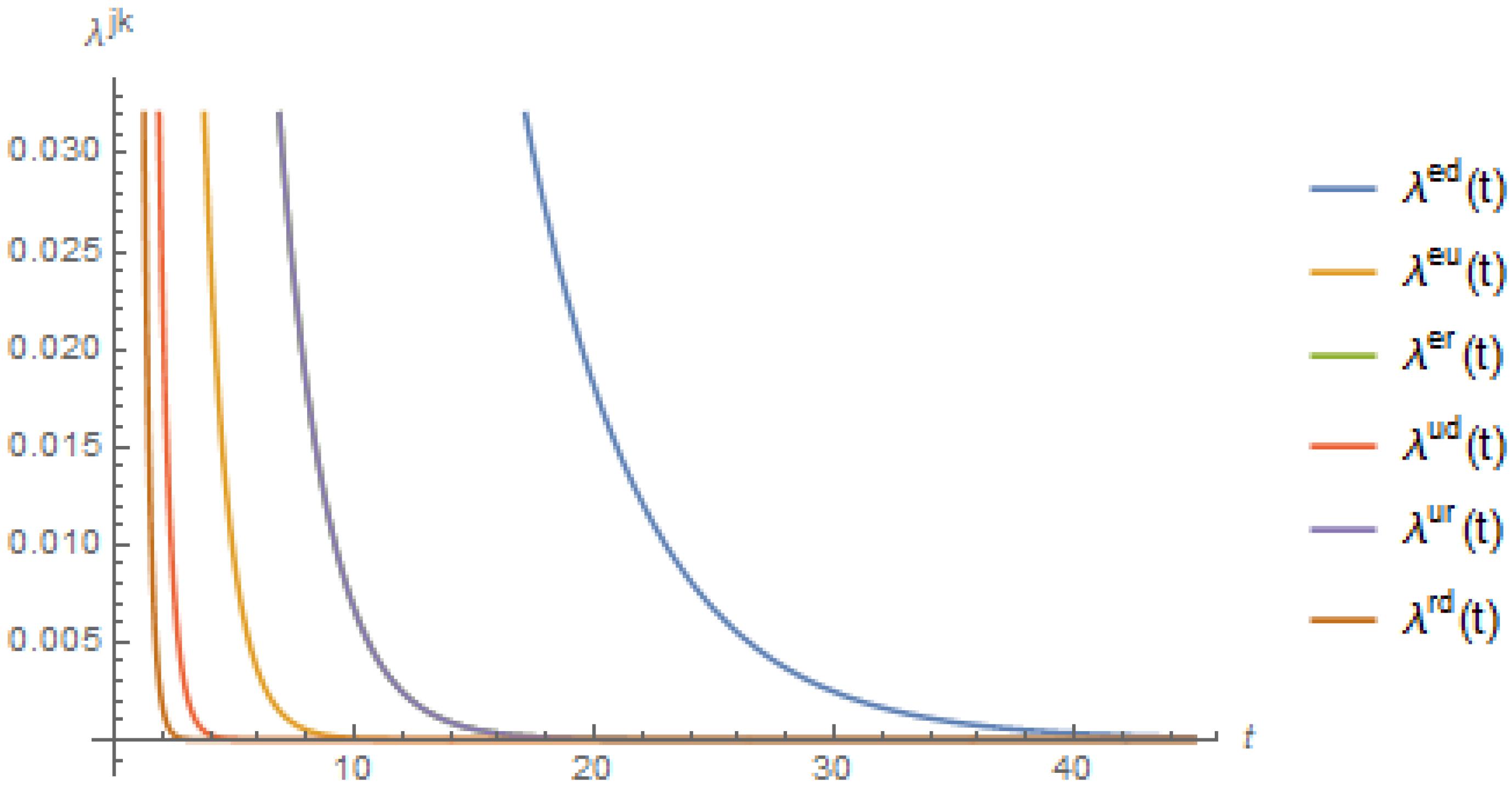
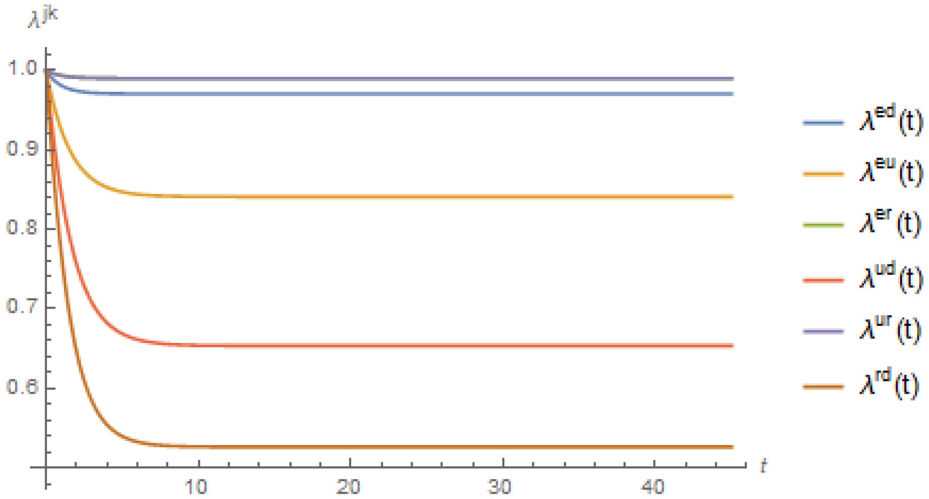
We illustrate the effect of non-zero jump coefficients in Figure 3, which shows the decrement probabilities of all states assuming the values in Table 1. We note the lower probability values for all states as the duration increased from 2 to 40. For the state $rd$, the probability value converged to zero at $t=2$, as opposed to the probability value for the same state converging to zero at $t=6$ under the CIR process, as depicted in Figure 4. A similar pattern was also shown by the decrement probability of all other states.

To highlight the quantitative effect of the shock events, we provide a numerical illustration of total reserves under eight combinations of the average jump-frequency parameters $\{{\rho }^{\left(ed\right)},{\rho }^{\left(eu\right)},{\rho }^{\left(er\right)},{\rho }^{\left(ud\right)},{\rho }^{\left(ur\right)},{\rho }^{\left(rd\right)}\}$ in

Table 2. Values of total reserves with various combinations of average jump frequency (rounded to 4 decimal places). The term Comp. denotes Component.

Combination of Average Jump Frequency	Comp. 1 ${\mathit{T}}_{\mathbf{1}}\mathbf{=}\mathbf{65}\mathbf{;}$ ${\mathit{T}}_{\mathbf{1}}\mathbf{=}\mathbf{70}$	Comp. 2 ${\mathit{T}}_{\mathbf{1}}\mathbf{=}\mathbf{65}\mathbf{;}$ ${\mathit{T}}_{\mathbf{1}}\mathbf{=}\mathbf{70}$	Comp. 3 ${\mathit{T}}_{\mathbf{1}}\mathbf{=}\mathbf{65}\mathbf{;}$ ${\mathit{T}}_{\mathbf{1}}\mathbf{=}\mathbf{70}$	Comp. 4 ${\mathit{T}}_{\mathbf{1}}\mathbf{=}\mathbf{65}\mathbf{;}$ ${\mathit{T}}_{\mathbf{1}}\mathbf{=}\mathbf{70}$	Comp. 5 ${\mathit{T}}_{\mathbf{1}}\mathbf{=}\mathbf{65}\mathbf{;}$ ${\mathit{T}}_{\mathbf{1}}\mathbf{=}\mathbf{70}$	Total Reserves ${\mathit{T}}_{\mathbf{1}}\mathbf{=}\mathbf{65}\mathbf{;}$ ${\mathit{T}}_{\mathbf{1}}\mathbf{=}\mathbf{70}$
${\rho }^{\left(ed\right)}=0,$ ${\rho }^{\left(eu\right)}=0,$ ${\rho }^{\left(er\right)}=0,$ ${\rho }^{\left(ud\right)}=0,$ ${\rho }^{\left(ur\right)}=0,$ ${\rho }^{\left(rd\right)}=0$	$0.0268;$ $0.0268$	$1.5123;$ $1.7983$	$0.0494;$ $0.0494$	$13.5308;$ $13.0327$	$0.6912;$ $0.8220$	$15.8106;$ $15.7292$
${\rho }^{\left(ed\right)}=1,$ ${\rho }^{\left(eu\right)}=0,$ ${\rho }^{\left(er\right)}=0,$ ${\rho }^{\left(ud\right)}=0,$ ${\rho }^{\left(ur\right)}=0,$ ${\rho }^{\left(rd\right)}=0$	$0.7658;$ $0.7713$	$1.2359;$ $1.4643$	$0.0398;$ $0.0398$	$11.0577;$ $10.6122$	$0.5649;$ $0.6693$	$13.6640;$ $13.5570$
${\rho }^{\left(ed\right)}=0,$ ${\rho }^{\left(eu\right)}=0,$ ${\rho }^{\left(er\right)}=0,$ ${\rho }^{\left(ud\right)}=3,$ ${\rho }^{\left(ur\right)}=0,$ ${\rho }^{\left(rd\right)}=0$	$0.0268;$ $0.0268$	$0.0507;$ $0.0507$	$0.1477;$ $0.1477$	$0.4534;$ $0.3672$	$0.0232;$ $0.0232$	$0.7017;$ $0.6156$
${\rho }^{\left(ed\right)}=0,$ ${\rho }^{\left(eu\right)}=0,$ ${\rho }^{\left(er\right)}=0,$ ${\rho }^{\left(ud\right)}=0,$ ${\rho }^{\left(ur\right)}=0,$ ${\rho }^{\left(rd\right)}=5$	$0.0268;$ $0.0268$	$1.5123;$ $1.7983$	$0.0494;$ $0.0494$	$0.0154;$ $0.0146$	$1.5119;$ $1.7980$	$3.1158;$ $3.6871$
${\rho }^{\left(ed\right)}=0,$ ${\rho }^{\left(eu\right)}=2,$ ${\rho }^{\left(er\right)}=0,$ ${\rho }^{\left(ud\right)}=0,$ ${\rho }^{\left(ur\right)}=0,$ ${\rho }^{\left(rd\right)}=0$	$0.0181;$ $0.0181$	$9.6481;$ $11.4474$	$0.3124;$ $0.3124$	$86.3251;$ $82.9605$	$4.4099;$ $5.2323$	$100.7137;$ $99.9708$
${\rho }^{\left(ed\right)}=0,$ ${\rho }^{\left(eu\right)}=0,$ ${\rho }^{\left(er\right)}=1,$ ${\rho }^{\left(ud\right)}=0,$ ${\rho }^{\left(ur\right)}=0,$ ${\rho }^{\left(rd\right)}=0$	$0.0200;$ $0.0200$	$0.9675;$ $1.1430$	$0.0308;$ $0.0308$	$8.6565;$ $8.2834$	$0.4422;$ $0.5224$	$10.1170;$ $9.9996$
${\rho }^{\left(ed\right)}=0,$ ${\rho }^{\left(eu\right)}=0,$ ${\rho }^{\left(er\right)}=0,$ ${\rho }^{\left(ud\right)}=0,$ ${\rho }^{\left(ur\right)}=1,$ ${\rho }^{\left(rd\right)}=0$	$0.0268;$ $0.0268$	$0.1656;$ $0.1657$	$0.0212;$ $0.0212$	$1.4821;$ $1.2005$	$0.0757;$ $0.0757$	$1.7715;$ $1.4899$
${\rho }^{\left(ed\right)}=1,$ ${\rho }^{\left(eu\right)}=2,$ ${\rho }^{\left(er\right)}=1,$ ${\rho }^{\left(ud\right)}=3,$ ${\rho }^{\left(ur\right)}=1,$ ${\rho }^{\left(rd\right)}=5$	$0.1276;$ $0.1276$	$0.1708;$ $0.1708$	$0.4133;$ $0.4133$	$0.0017;$ $0.0014$	$0.1707;$ $0.1708$	$0.8842;$ $0.8838$

. The highest total reserves ($\$100.7137$) was given by the combination $\{{\rho }^{\left(ed\right)},{\rho }^{\left(eu\right)},{\rho }^{\left(er\right)},{\rho }^{\left(ud\right)},{\rho }^{\left(ur\right)},{\rho }^{\left(rd\right)}\}=\{0,2,0,0,0,0\}$, which returned the highest unemployed/disabled probability in components 2–5. It can be also noted that ${\kappa }_G^{\left(u\right)}$ and ${\kappa }_G^{\left(r\right)}$, that is, the unemployment/disabled benefit ($\$9.6481$, component 2) and age pension benefit ($$86.3251$, component 4), were the highest paid by a government social welfare system. We recall that component 2 represents the continuous annuity payment paid to individuals who are alive but permanently unemployed/disabled between times $t_1$ and $T_1$, while component 4 is the continuous annuity payment to an individual who had become permanently unemployed/disabled between $t_1$ and $T_1$ and who survived from $T_1$ until the maximum age $T_2$. The analyses of other combinations of $\{{\rho }^{\left(ed\right)},{\rho }^{\left(eu\right)},{\rho }^{\left(er\right)},{\rho }^{\left(ud\right)},{\rho }^{\left(ur\right)},{\rho }^{\left(rd\right)}\}$ are given by points 1–7:

• For the case of zero jumps (i.e., $\{{\rho }^{\left(ed\right)},{\rho }^{\left(eu\right)},{\rho }^{\left(er\right)},{\rho }^{\left(ud\right)},{\rho }^{\left(ur\right)},{\rho }^{\left(rd\right)}\}=\{0,0,0,0,0,0\}$), the employment probability in component 1 increased (on the other hand, the unemployment/disabled probability for components 2–5 decreased). Thus, the payments of components 2–4 were lower than for their counterpart (i.e., the combination $\{0,2,0,0,0,0\}$), and the payment of component 1 was also higher. Overall, the total reserves decreased to $\$15.8106$.
• For the combination $\{1,0,0,0,0,0\}$, the non-zero average jump frequency in the transition intensity from Employed to Death resulted in higher mortality in component 1 and a lower survival probability for components 2–4, resulting in a higher payment of immediate death benefits while still in the Employed state and lower payments for components 2–5 than in the zero-jumps scenario. Overall, the total reserve decreased to $\$13.6640$.
• While the combination $\{0,0,0,3,0,0\}$ did not affect component 1, the numerical effect showed a lower survival probability for components 2, 4, and 5, as well as higher mortality in component 3. These effects translated into lower payments of components 2, 4, and 5, as well as a higher payment for component 3 than for its counterpart $\{0,0,0,0,0,0\}$. Overall, the total reserves decreased, and we had $\$0.7017$.
• The non-zero average jump frequency in the transition intensity from Retired to Death, as shown by the combination $\{0,0,0,0,0,5\}$, resulted in a lower survival probability in component 4 as well as higher mortality in component 5. Although the combination did not affect components 1–3, these were then translated into a lower payment for component 4 and a higher payment for component 5, the $\{0,0,0,0,0,0\}$ combination. Overall, the total reserves decreased, and we had $\$3.1158$.
• Under the combination $\{0,0,1,0,0,0\}$, the non-retired probability while in the state Employed became lower in all components. Hence, the payments of all components were lower than for the all-zero jump-frequency combination $\{0,0,0,0,0,0\}$, resulting in a slightly lower total-reserves amount of $\$10.1170$.
• The combination $\{0,0,0,0,1,0\}$ affected only components 2–5 and had no effect on component 1. The lower non-retired probability of the Unemployed/Disabled state then translated into a lower payment than for the $\{0,0,0,0,0,0\}$ combination for components 2–5. Overall, the total reserves decreased to $\$1.7715$.
• For a combination with non-zero jump frequency for all states, such as $\{1,2,1,3,1,5\}$, the payments for components 1 and 3 were higher than for its counterpart (i.e., the all-zero average jump frequency $\{0,0,0,0,0,0\}$); this was attributable to higher mortality intensities. Simultaneously, the annuity payments for components 2 and 4 were lower than for their counterpart. Component 5 became lower as the survival probability and the non-retired probability from the Employed/Unemployed state became lower; thus the payment for component 5 was lower than for its counterpart. Overall, the total reserves decreased to $\$0.8842$.

The above analyses imply that when mortality rates are low (as in the combination $\{0,0,0,0,0,0\}$), as ${\rho }^{\left(eu\right)}$ increases, we observe higher annuity values for the states Unemployed/Disabled (component 2) and Retired (component 4). We also notice that when the currently employed individual was more likely to become unemployed/disabled, as in the combination $\{0,2,0,0,0,0\}$, the total reserves of the life insurance and social benefit scheme was approximately 6.4 times higher than in the low-mortality-rate environment: to wit, the total-reserves value increased to $\$100.7137$ from $\$15.8106$ (for $T_1=65$) and to $\$99.9708$ from $\$15.7292$ (for $T_1=70$). We also note that in comparison with the combination $\{1,2,1,3,1,5\}$, for which each state had a higher transition intensity (hence a higher chance of leaving the current state and not coming back), the total-reserves values under the low-mortality environment were approximately 18 times higher, that is, a total-reserves value of $\$15.8106$ as opposed to $\$0.8842$ (for $T_1=65$) and $\$15.7292$ as opposed to $\$0.8838$ (for $T_1=70$).

By raising the retirement age, we would see an increase in the government’s tax revenue as long as a sufficient unemployment rate is maintained. However, parallel with the findings by public economists (see Staubli and Zweim (2013) and references within), our numerical example shows that increasing the retirement age has a spillover effect that would increase government expenses for other social insurance programs, such as the unemployment/disability insurance scheme. This can be seen from Table 2, where for all combinations, component 2 (unemployment/disability annuity) showed higher annuity payments and component 4 (government expenses for age pension) decreased as the retirement age $T_1$ increased from 65 to 70.

The comparison clearly shows the numerical effect of a government policy to delay retirement age in terms of the extra monetary burden shouldered by policy makers if involuntary early retirees increase as a result of unemployment/disability. Hence, it may become necessary for individuals to count on government unemployment/disability benefits for a longer period before accessing their occupational pension funds. The need for more reserves could be made worse during periods of economic downturn, when there is an increase in the number of discouraged workers (see Topel 1983 and Topel 1984), or under conditions in which some individuals simply prefer to take benefits for a prolonged period rather than working until the extended retirement age (see Meyer 1990).

4.2. Sensitivity Analysis

We are now interested in exploring the effect of changes in retirement age on components and total reserves. We conducted a sensitivity analyses to examine the quantitative effect of increasing the retirement age $T_1$ from 65 to 67, 70, 72, and 75, with $t_1=45$ and $T_2=85$. We varied the jump-size parameter $\alpha$, average frequency of jump occurrences $\rho$, and the diffusion parameter $\sigma$ in the state ($eu$) that affects all components. We also reconfirmed the spillover effect on the unemployment/disability insurance pool due to the government policy of delaying retirement age.

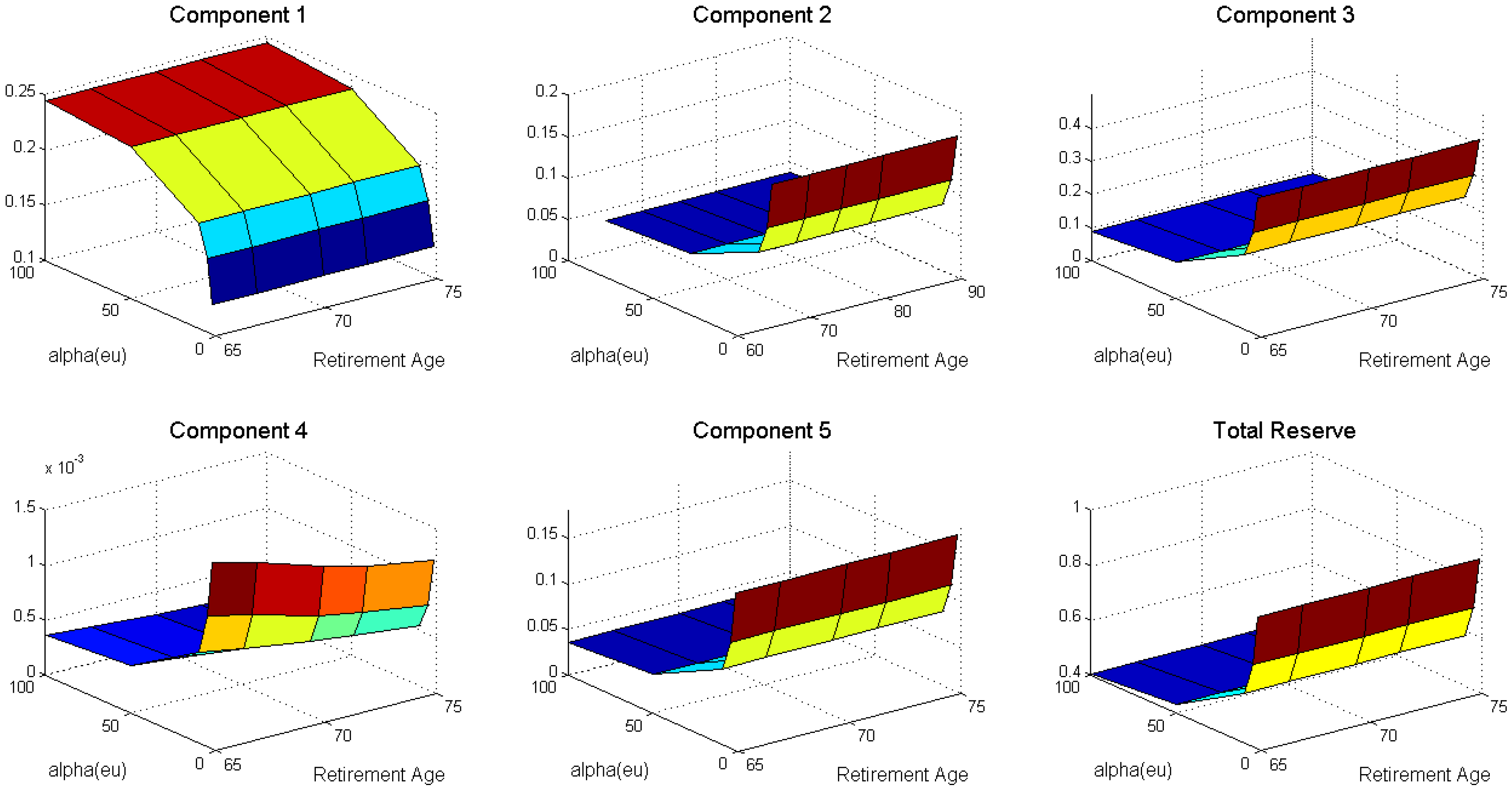
As we changed the jump-size parameter ${\alpha }^{\left(eu\right)}$, we noted that the total-reserves amount decreased as the jump-size parameter ${\alpha }^{\left(eu\right)}$ increased, as shown in Figure 5. An increase in the jump-size parameter will reduce the exponential average $\frac{1}{{\alpha }^{\left(eu\right)}},$ hence causing the employment probability to rise. Therefore we can expect to have a lower amount for components 2–5 being set aside for the individuals and a higher amount for death benefits payments because of an increasing employment probability, as represented by component 1.

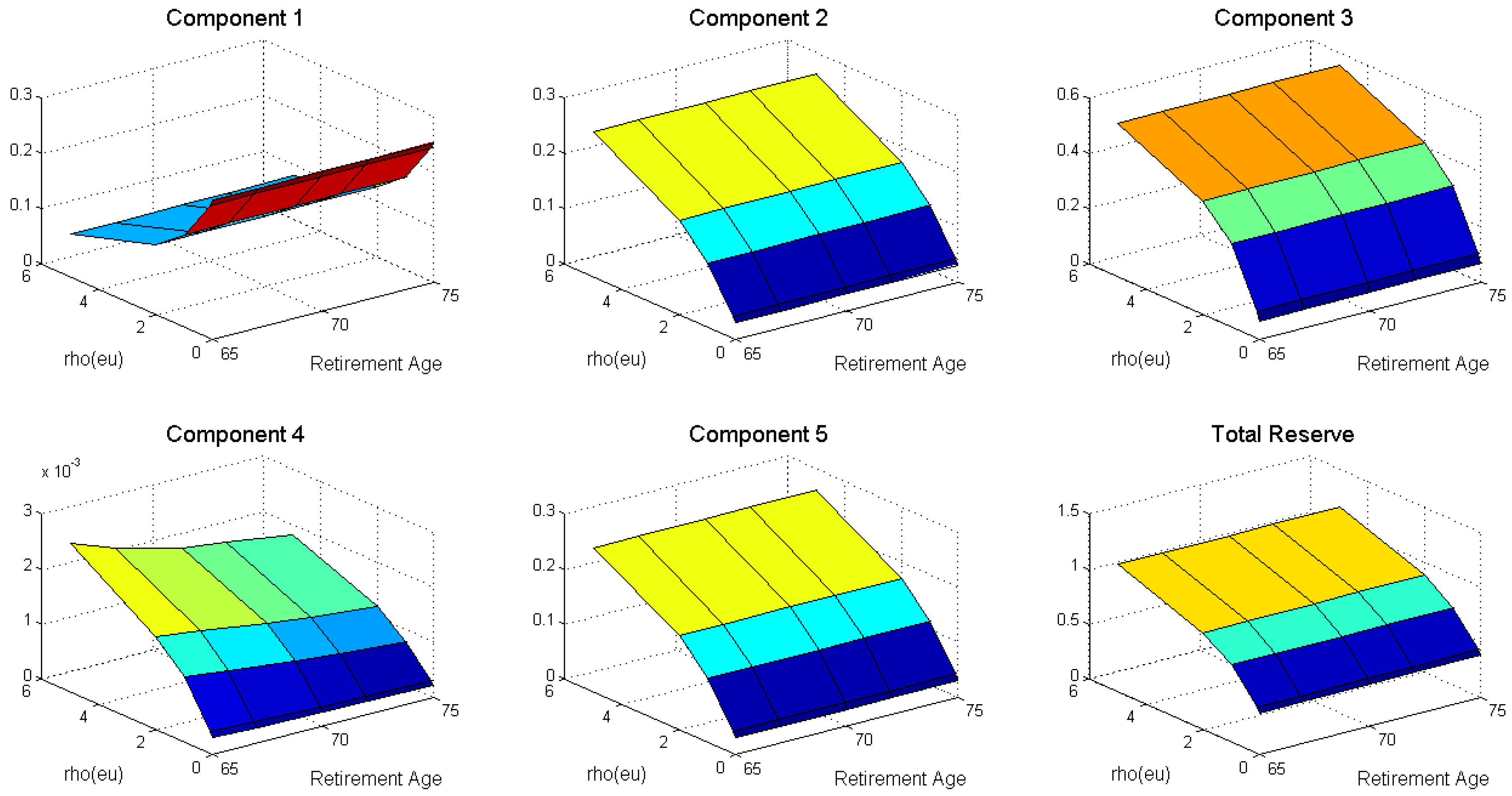
Figure 6 reveals that the total reserves increased as we increased the average frequency of jumps from Employed $(e)$ to Unemployed/Disabled $(u)$ (i.e., ${\rho }^{\left(eu\right)}$). The sources of changes were components 2–5, as these are the parts of the reserves that are affected by a decreasing employment probability. An increase in ${\rho }^{\left(eu\right)}$ would result in a higher transition intensity from the state Employed to the state Unemployed/Disabled, thereby decreasing the employment probability in component 1 and increasing the intensity to the state Unemployed/Disabled while in the state Employed for components 2–5. This implies that an increase in the average jump frequency will reduce the employment probability while in the state Employed. Thus, the social insurance provider will require a higher reserve amount to ensure that benefits are appropriately paid to beneficiaries upon transition into, and while in, the other three states.

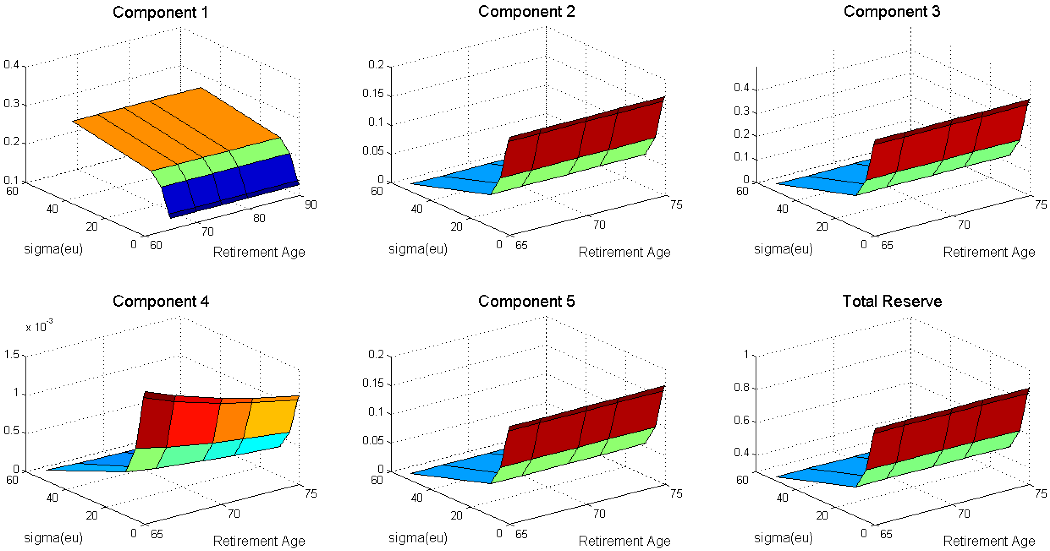
We also note that the total-reserves amount decreased as the diffusion parameter ${\sigma }^{\left(eu\right)}$ increased, as shown in Figure 7. An increase in the diffusion parameter will increase the employment probability, and thereby we can expect to allocate a higher amount of insurance to be paid to the individuals, as represented by component 1. Simultaneously, an increase in the employment probability implies a decrease in employment probability; we see that components 2–5 showed a decreasing pattern as a function of ${\sigma }^{\left(eu\right)}$.

Concerning the duration of life and the social insurance scheme, the values of the total reserves decreased as the retirement age $T_1$ increased from 65 to 67, 70, 72, and 75 for all three parameters (as shown in Figure 5, Figure 6 and Figure 7). As seen in the previous subsection, the pension annuity paid to individuals who had become permanently unemployed/disabled between ages 45 and $T_1$ but who survived until the maximum age $T_2=85$ from $T_1$ (i.e., component 4) also decreased. We also note that component 2 increased for all three parameters when we increased the retirement age $T_1$.

Keeping the maximum survival age fixed at 85 years old, our computation also indicated that the total reserves changed by $-63\%$ as $\alpha$ increased from 2 to 100 and by $-54\%$ as $\sigma$ increased from 0.5 to 50. On the other hand, the total reserves changed by $+203\%$ as $\rho$ increased from 0.01 to 5. Maintaining the variation in parameters, as the retirement age increased from 65 to 75 years old, the total reserves decreased by 3–6 basis points (bps) as a result of the increase in $\alpha$, by 3–8 bps as a result of the increase in $\rho$, and by 1–6 bps as a result of the increase in $\sigma$.

It is of interest to look at the effect of increasing the maximum survival age $T_2$ from 85 to 90, 95, 100, and 105 by changing the average jump-size parameter $\alpha$, jump-frequency occurrence $\rho$, and diffusion parameters $\sigma$ for the transition intensity from Employed to Unemployed/Disabled with $t_1=45$ and $T_1=85$, as the changes will be reflected in all components. Additionally, it is also of interest to examine the applicability of the model on a set of mortality and market data, which we leave as the next objective of further research.

5. Conclusions

While improved longevity is considered a blessing to individuals, it may cause a financial burden to a government if not appropriately managed. As providers of social insurance schemes, many governments consider increasing the retirement age as part of pension reforms. However, to understand the effect of this change, we need to examine how people react to the fact that they have to work longer until reaching the increased retirement age before they gain access to their occupational pension fund. In particular, individuals may react by taking government unemployment/disability benefits rather than working until the increased retirement age, thus offsetting the increase in the income tax revenues for the unemployment/disability benefits. In this study, therefore, we assessed the burden to the policy makers/government if working individuals become reliant on unemployment/disability benefits instead of working until reaching a retirement age that is higher than usual. The assessment was based on a hierarchical four-state Markov chain supporting a life insurance and pension annuity model, which was essential to probe the impact of delaying retirement age.

We modeled the interstate transition intensities using the multivariate jump-diffusion process and used its Laplace transform to compute the decrement probability. Assuming independence and a deterministic interest rate, we then evaluated the prospective reserves for a social benefit scheme for a nation. We utilized the CIR process with jump diffusion after taking into account the advantage it presented over the usual CIR process without jumps. In addition to demonstrating the vast difference between the reserves amount under the jump-diffusion and CIR environment, we also conducted sensitivity analyses by changing the relevant parameters in the unemployed/disabled and retired states, which are the average jump size $\alpha$, the jump frequency $\rho$, and the diffusion parameters $\sigma$. Our numerical findings are in line with Staubli and Zweim (2013), whereby an increase in the retirement age would result in a spillover effect on unemployment/disability benefits.