Credit Risk Analysis Using Machine and Deep Learning Models †

Abstract
1. Introduction
2. A Unified Presentation of Models
2.1. Elastic Net
- Linear regression: The response belongs to R. Thus, we use the model (1). In that case, the parameter of interest is , and another set of parameters to be estimated is . The existence of correlation must be considered to verify if the values used for those parameters are efficient or not.
- Logistic regression: The response is binary (0 or 1). In that case, the logistic regression represents the conditional probabilities through a nonlinear function of the predictors where , then we solve:
- Multinomial regression: The response has possibilities. In that case, the conditional probability is2:
2.2. Random Forest Modeling
2.3. A Gradient Boosting Machine
2.4. Deep Learning
3. The Criteria
4. Data and Models
4.1. The Data
4.2. The Models
4.2.1. Precisions on the Parameters Used to Calibrate the Models
- The Logistic regression model M1: To fit the logistic regression modeling, we use the elastic net: logistic regression and regularization functions. This means that the parameter in Equation (1) and Equation (2) can change. In our exercise, in Equation (3) (the fitting with provides the same results) and (this very small value means that we have privileged the ridge modeling) are used.
- The random forest model M2: Using Equation (6) to model the random forest approach, we choose the number of trees (this choice permits testing the total number of features), and the stopping criterion is equal to . If the process converges quicker than expected, the algorithm stops, and we use a smaller number of trees.
- The gradient boosting model M3: To fit this algorithm, we use the logistic binomial log-likelihood function: , for classification, and the stopping criterion is equal to . We need a learning rate that is equal to . At each step, we use a sample rate corresponding to 70% of the training set used to fit each tree.
- Deep learning: Four versions of the deep learning neural networks models with stochastic gradient descent have been tested.
- D1: For this model, two hidden layers and 120 neurons have been implemented. This number depends on the number of features, and we take 2/3 of this number. It corresponds also to the number used a priori with the random forest model and gives us a more comfortable design for comparing the results.
- D2: Three hidden layers have been used, each composed of 40 neurons, and a stopping criteria equal to has been added.
- D3: Three hidden layers with 120 neurons each have been tested. A stopping criteria equal to and the and regularization functions have been used.
- D4: Given that there are many parameters that can impact the model’s accuracy, hyper-parameter tuning is especially important for deep learning. Therefore, in this model, a grid of hyper-parameters has been specified to select the best model. The hyper0parameters include the drop out ratio, the activation functions, the and regularization functions and the hidden layers. We also use a stopping criterion. The best model’s parameters yields a dropout ratio of 0, , , hidden layers = , and the activation function is the rectifier ( if , if not .
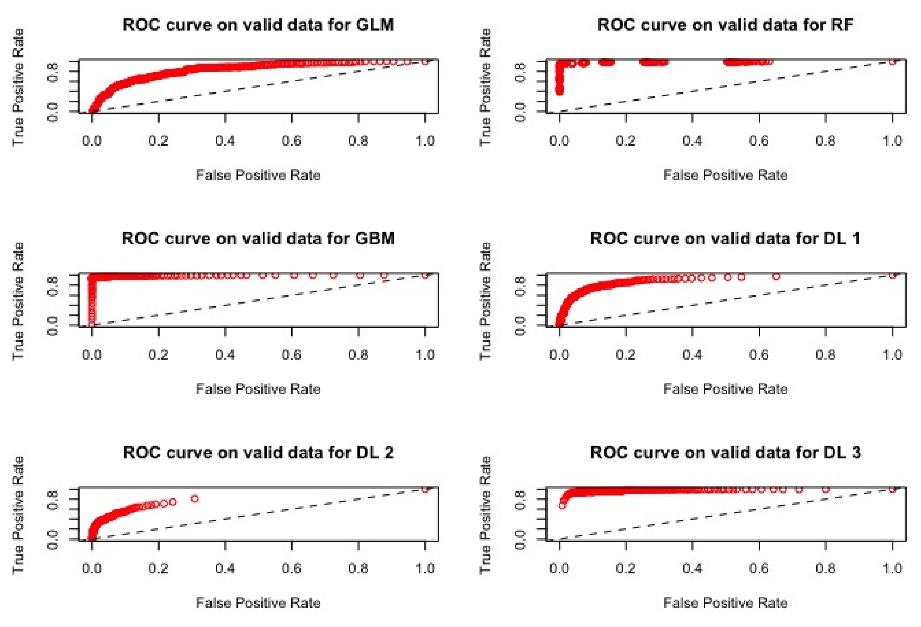
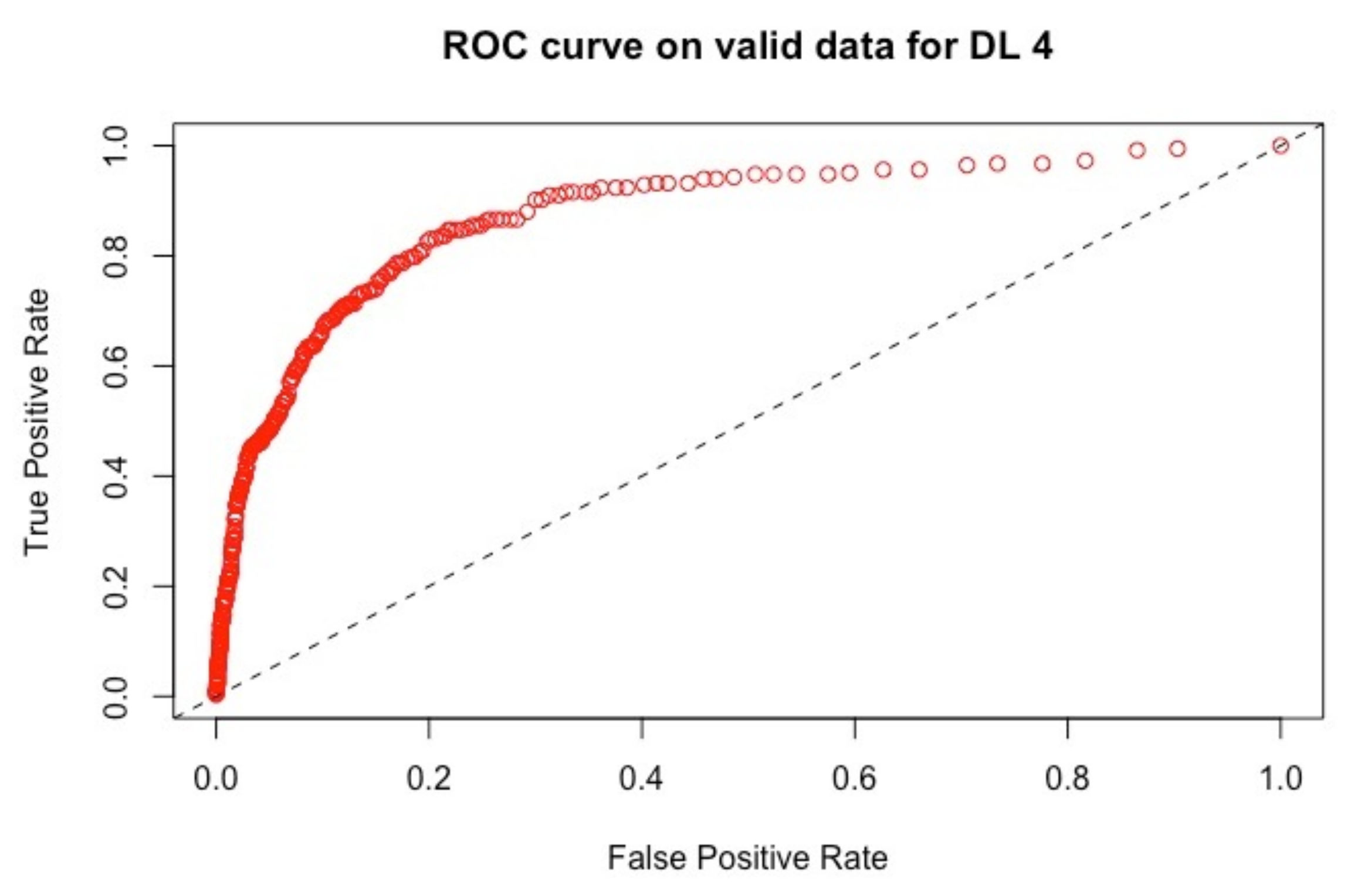
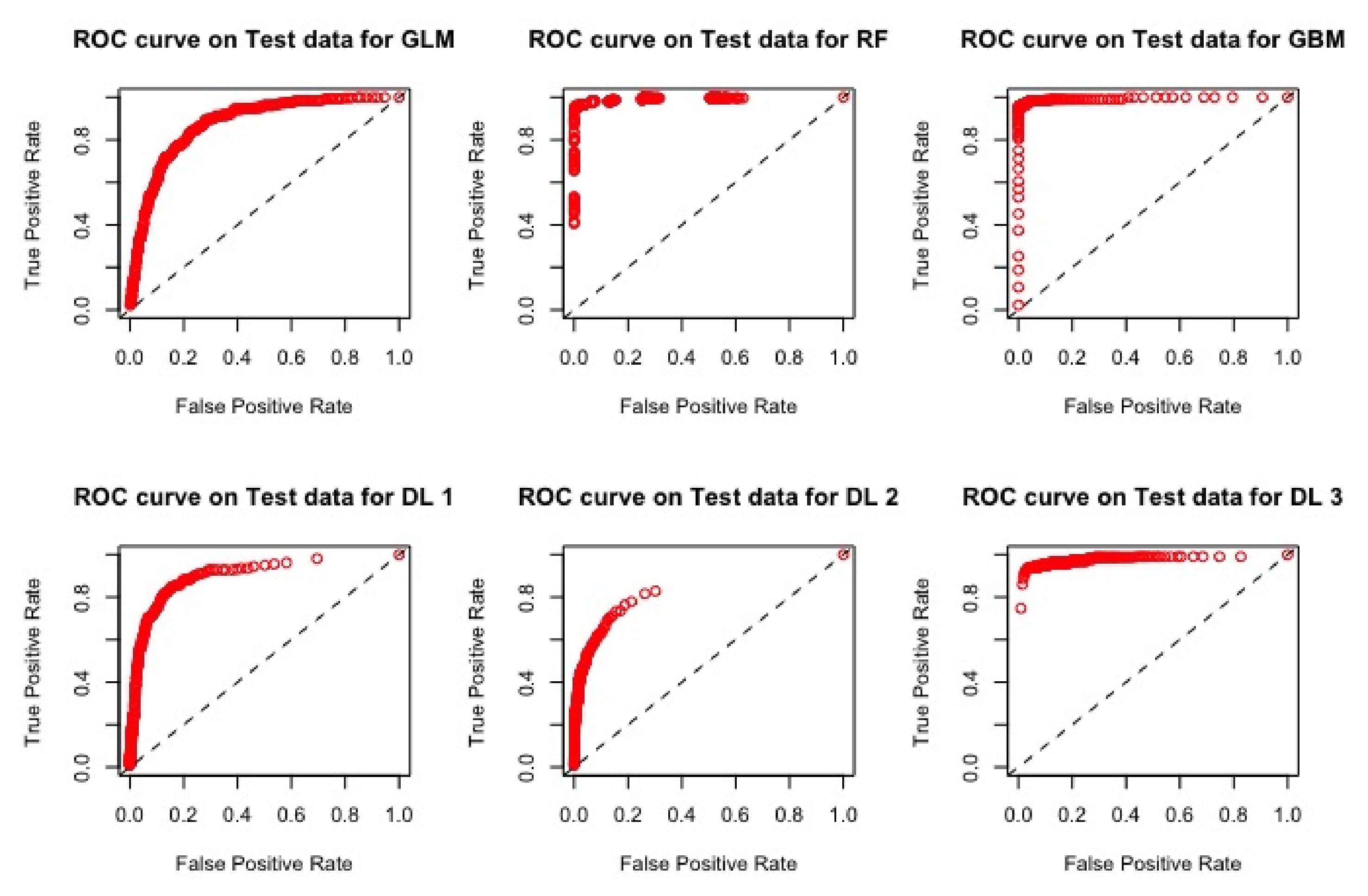
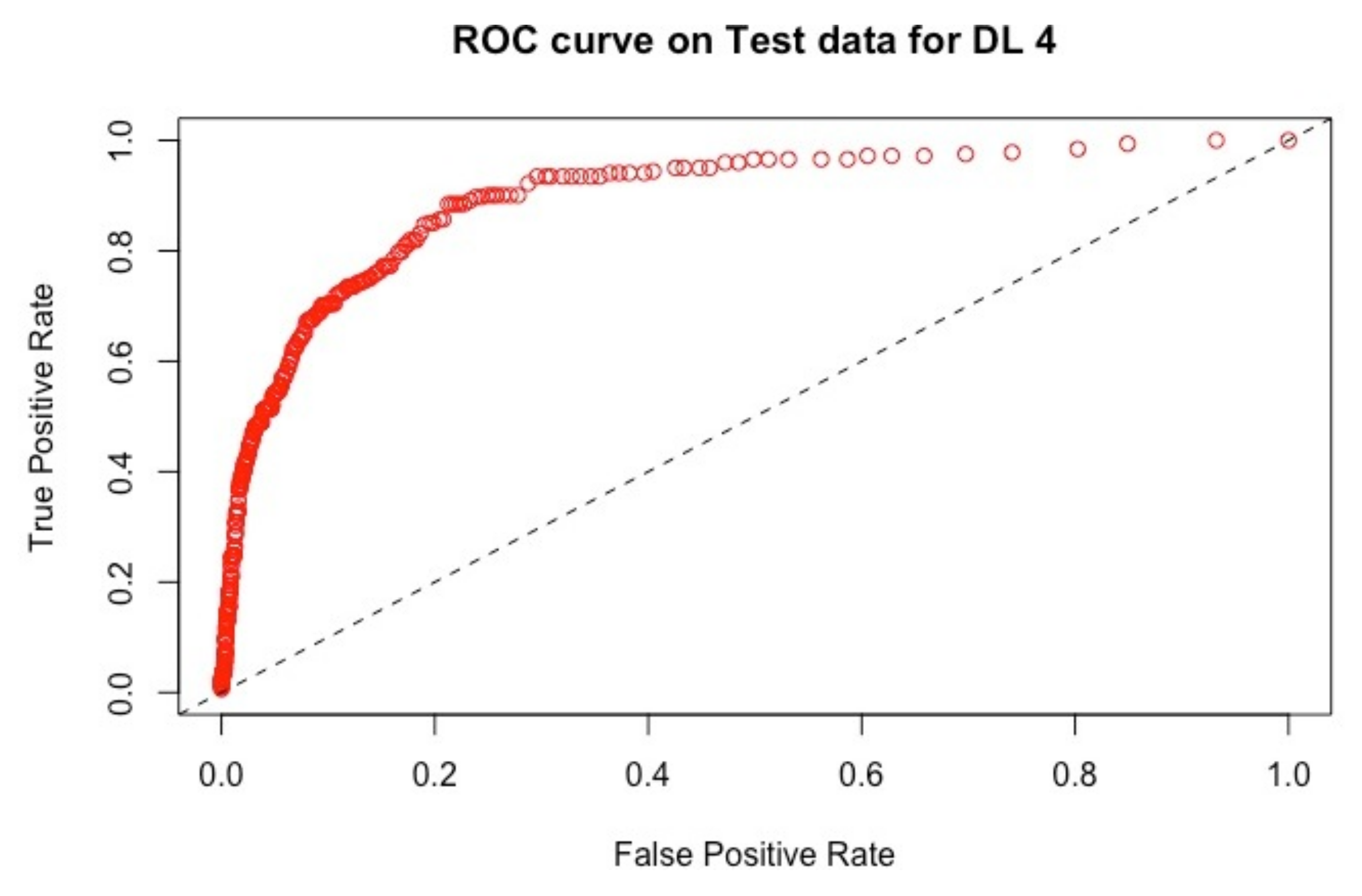
4.2.2. Results
5. Conclusions
Acknowledgments
Author Contributions
Conflicts of Interest
References
- Angelini, Eliana, Giacomo di Tollo, and Andrea Roli. 2008. A neural network approach for credit risk evaluation. The Quarterly Review of Economics and Finance 48: 733–55. [Google Scholar] [CrossRef]
- Anisha Arora, Arno Candel, Jessica Lanford, Erin LeDell, and Viraj Parmar. 2015. The Definitive Performance Tuning Guide for H2O Deep Learning. Leghorn St. Mountain View, CA, USA: H2O.ai, Inc. [Google Scholar]
- Bahrammirzaee, Arash. 2010. A comparative survey of artificial intelligence applications in finance: Artificial neural networks, expert system and hybrid intelligent systems. Neural Computing and Applications 19: 1165–95. [Google Scholar] [CrossRef]
- Balzer, Robert. 1985. A 15 year perspective on automatic programming. IEEE Transactions on Software Engineering 11: 1257–68. [Google Scholar] [CrossRef]
- Biau, Gérard. 2012. Analysis of a random forests model. Journal of Machine Learning Research 13: 1063–95. [Google Scholar]
- Breiman, Leo. 2000. Some Infinity Theory for Predictors Ensembles. Technical Report. Berkeley: UC Berkeley, vol. 577. [Google Scholar]
- Breiman, Leo. 2004. Consistency for a Sample Model of Random Forests. Technical Report 670. Berkeley: UC Berkeley, vol. 670. [Google Scholar]
- Butaru, Florentin, Qingqing Chen, Brian Clark, Sanmay Das, Andrew W. Lo, and Akhtar Siddique. 2016. Risk and risk management in the credit card industry. Journal of Banking and Finance 72: 218–39. [Google Scholar] [CrossRef]
- Ling, Charles X., and Chenghui Li. 1998. Data Mining for Direct Marketing Problems and Solutions. Paper presented at International Conference on Knowledge Discovery from Data (KDD 98). New York City, August 27–31; pp. 73–79. [Google Scholar]
- Chawla, Nitesh V., Kevin W. Bowyer, Lawrence O. Hall, and W. Philip Kegelmeyer. 2002. Smote: Synthetic minority over-sampling technique. Journal of Artificial Intelligence Research 16: 321–57. [Google Scholar]
- CNIL. 2017. La loi pour une république numérique: Concertation citoyenne sur les enjeux éthiques lies à la place des algorithmes dans notre vie quotidienne. In Commission nationale de l’informatique et des libertés. Montpellier: CNIL. [Google Scholar]
- Deville, Yves, and Kung-Kiu Lau. 1994. Logic program synthesis. Journal of Logic Programming 19: 321–50. [Google Scholar] [CrossRef]
- Pierre Geurts, Damien Ernst, and Louis Wehenkel. 2006. Extremely randomized trees. Machine Learning 63: 3–42. [Google Scholar] [CrossRef]
- Fan, Jianqing, and Runze Li. 2001. Variable selection via nonconcave penalized likelihood and its oracle properties. Journal of the American Statistical Society 96: 1348–60. [Google Scholar] [CrossRef]
- Friedman, Jerome, Trevor Hastie, and Rob Tibshirani. 2001. The elements of statistical learning. Springer Series in Statistics 1: 337–87. [Google Scholar]
- Friedman, Jerome, Trevor Hastie, and Rob Tibshirani. 2010. Regularization paths for generalized linear models via coordinate descent. Journal of Statistical Software 33: 1. [Google Scholar] [CrossRef] [PubMed]
- Friedman, Jerome H. 2001. Greedy function approximation: A gradient boosting machine. The Annals of Statistics 29: 1189–232. [Google Scholar] [CrossRef]
- Galindo, Jorge, and Pablo Tamayo. 2000. Credit risk assessment using statistical and machine learning: Basic methodology and risk modeling applications. Computational Economics 15: 107–43. [Google Scholar] [CrossRef]
- Gastwirth, Joseph L. 1972. The estimation of the lorenz curve and the gini index. The Review of Economics and Statistics 54: 306–16. [Google Scholar] [CrossRef]
- GDPR. 2016. Regulation on the Protection of Natural Persons with Regard to the Processing of Personal Data and on the Free Movement of Such Data, and Repealing Directive 95/46/EC (General Data Protection Regulation). EUR Lex L119. Brussels: European Parliament, pp. 1–88. [Google Scholar]
- Gedeon, Tamás D. 1997. Data mining of inputs: Analyzing magnitude and functional measures. International Journal of Neural Systems 8: 209–17. [Google Scholar] [CrossRef] [PubMed]
- Genuer, Robin, Jean-Michel Poggi, and Christine Tuleau. 2008. Random Forests: Some Methodological Insights. Research Report RR-6729. Paris: INRIA. [Google Scholar]
- Hinton, Geoffrey E., and Ruslan R. Salakhutdinov. 2006. Reducing the dimensionality of data with neural networks. Science 313: 504–7. [Google Scholar] [CrossRef] [PubMed]
- Siegelmann, Hava T., and Eduardo D. Sontag. 1991. Turing computability with neural nets. Applied Mathematics Letters 4: 77–80. [Google Scholar] [CrossRef]
- Huang, Zan, Hsinchun Chen, Chia-Jung Hsu, Wun-Hwa Chen, and Soushan Wu. 2004. Credit rating analysis with support vector machines and neural networks: A market comparative study. Decision Support Systems 37: 543–58. [Google Scholar] [CrossRef]
- Kenett, Ron S., and Silvia Salini. 2011. Modern analysis of customer surveys: Comparison of models and integrated analysis. Applied Stochastic Models in Business and Industry 27: 465–75. [Google Scholar] [CrossRef]
- Khandani, Amir E., Adlar J. Kim, and Andrew W. Lo. 2010. Consumer credit-risk models via machine-learning algorithms. Journal of Banking and Finance 34: 2767–87. [Google Scholar] [CrossRef]
- Kubat, Miroslav, Robert C. Holte, and Stan Matwin. 1999. Machine learning in the detection of oil spills in satellite radar images. Machine Learning 30: 195–215. [Google Scholar] [CrossRef]
- Kubat, Miroslav, and Stan Matwin. 1997. Addressing the curse of imbalanced training sets: One sided selection. Paper presented at Fourteenth International Conference on Machine Learning. San Francisco, CA, USA, July 8–12; pp. 179–186. [Google Scholar]
- Lerman, Robert I., and Shlomo Yitzhaki. 1984. A note on the calculation and interpretation of the gini index. Economic Letters 15: 363–68. [Google Scholar] [CrossRef]
- Menardi, Giovanna, and Nicola Torelli. 2011. Training and assessing classification rules with imbalanced data. Data Mining and Knowledge Discovery 28: 92–122. [Google Scholar] [CrossRef]
- Mladenic, Dunja, and Marko Grobelnik. 1999. Feature selection for unbalanced class distribution and naives bayes. Paper presented at 16th International Conference on Machine Learning. San Francisco, CA, USA, June 27–30; pp. 258–267. [Google Scholar]
- Raileanu, Laura Elena, and Kilian Stoffel. 2004. Theoretical comparison between the gini index and information gain criteria. Annals of Mathematics and Artificial Intelligence 41: 77–93. [Google Scholar] [CrossRef]
- Schmidhuber, Jurgen. 2014. Deep Learning in Neural Networks: An Overview. Technical Report IDSIA-03-14. Lugano: University of Lugano & SUPSI. [Google Scholar]
- Schölkopf, Bernhard, Christopher J. C. Burges, and Alexander J. 1998. Advances in Kernel Methods—Support Vector Learning. Cambridge: MIT Press, vol. 77. [Google Scholar]
- Seetharaman, A, Vikas Kumar Sahu, A. S. Saravanan, John Rudolph Raj, and Indu Niranjan. 2017. The impact of risk management in credit rating agencies. Risks 5: 52. [Google Scholar] [CrossRef]
- Sirignano, Justin, Apaar Sadhwani, and Kay Giesecke. 2018. Deep Learning for Mortgage Risk. Available online: https://ssrn.com/abstract=2799443 (accessed on 9 February 2018).
- Tibshirani, Robert. 1996. Regression shrinkage and selection via the lasso. Journal of the Royal Statistical Society, Series B 58: 267–88. [Google Scholar]
- Tibshirani, Robert. 2011. Regression shrinkage and selection via the lasso:a retrospective. Journal of the Royal Statistical Society, Series B 58: 267–88. [Google Scholar]
- Vapnik, Vladimir. 1995. The Nature of Statistical Learning Theory. Berlin: Springer. [Google Scholar]
- Yitzhaki, Shlomo. 1983. On an extension of the gini inequality index. International Economic Review 24: 617–28. [Google Scholar] [CrossRef]
- Zou, Hui. 2006. The adaptive lasso and its oracle properties. Journal of the American Statistical Society 101: 1418–29. [Google Scholar] [CrossRef]
- Zou, Hui, and Trevor Hastie. 2005. Regulation and variable selection via the elastic net. Journal of the Royal Statistical Society 67: 301–20. [Google Scholar] [CrossRef]
| 1. | There exist a lot of other references concerning Lasso models; thus, this introduction does not consider all the problems that have been investigated concerning this model. We provide some more references noting that most of them do not have the same objectives as ours. The reader can read with interest Fan and Li (2001), Zhou (2006) and Tibschirani (2011). |
| 2. | Here, T stands for transpose |
| 3. | As soon as the AUC is known, the Gini index can be obtained under specific assumptions |
| 4. | In medicine, it corresponds to the probability of the true negative |
| 5. | In medicine, corresponding to the probability of the true positive |
| 6. | The code implementation in this section was done in ‘R’. The principal package used is H2o.ai Arno et al. (2015). The codes for replication and implementation are available at https://github.com/brainy749/CreditRiskPaper. |


| Models | AUC | RMSE |
|---|---|---|
| M1 | 0.842937 | 0.247955 |
| M2 | 0.993271 | 0.097403 |
| M3 | 0.994206 | 0.041999 |
| D1 | 0.902242 | 0.120964 |
| D2 | 0.812946 | 0.124695 |
| D3 | 0.979357 | 0.320543 |
| D4 | 0.877501 | 0.121133 |
| Models | AUC | RMSE |
|---|---|---|
| M1 | 0.876280 | 0.245231 |
| M2 | 0.993066 | 0.096683 |
| M3 | 0.994803 | 0.044277 |
| D1 | 0.904914 | 0.114487 |
| D2 | 0.841172 | 0.116625 |
| D3 | 0.975266 | 0.323504 |
| D4 | 0.897737 | 0.113269 |
| M1 | M2 | M3 | D1 | D2 | D3 | D4 | |
|---|---|---|---|---|---|---|---|
| X1 | A1 | A11 | A11 | A25 | A11 | A41 | A50 |
| X2 | A2 | A5 | A6 | A6 | A32 | A42 | A7 |
| X3 | A3 | A2 | A17 | A26 | A33 | A43 | A51 |
| X4 | A4 | A1 | A18 | A27 | A34 | A25 | A52 |
| X5 | A5 | A9 | A19 | A7 | A35 | A44 | A53 |
| X6 | A6 | A12 | A20 | A28 | A36 | A45 | A54 |
| X7 | A7 | A13 | A21 | A29 | A37 | A46 | A55 |
| X8 | A8 | A14 | A22 | A1 | A38 | A47 | A56 |
| X9 | A9 | A15 | A23 | A30 | A39 | A48 | A57 |
| X10 | A10 | A16 | A24 | A31 | A40 | A49 | A44 |
| TYPE | METRIC |
|---|---|
| EBITDA | EBITDA/FINACIAL EXPENSES |
| EBITDA/Total ASSETS | |
| EBITDA/EQUITY | |
| EBITDA/SALES | |
| EQUITY | EQUITY/TOTAL ASSETS |
| EQUITY/FIXED ASSETS | |
| EQUITY/LIABILITIES | |
| LIABILITIES | LONG-TERM LIABILITIES/TOTAL ASSETS |
| LIABILITIES/TOTAL ASSETS | |
| LONG TERM FUNDS/FIXED ASSETS | |
| RAW FINANCIALS | LN (NET INCOME) |
| LN(TOTAL ASSETS) | |
| LN (SALES) | |
| CASH-FLOWS | CASH-FLOW/EQUITY |
| CASH-FLOW/TOTAL ASSETS | |
| CASH-FLOW/SALES | |
| PROFIT | GROSS PROFIT/SALES |
| NET PROFIT/SALES | |
| NET PROFIT/TOTAL ASSETS | |
| NET PROFIT/EQUITY | |
| NET PROFIT/EMPLOYEES | |
| FLOWS | (SALES (t) −SALES (t−1))/ABS(SALES (t−1)) |
| (EBITDA (t) −EBITDA (t−1))/ABS(EBITDA (t−1)) | |
| (CASH-FLOW (t) −CASH-FLOW (t−1))/ABS(CASH-FLOW (t−1)) | |
| (EQUITY (t) − EQUITY (t−1))/ABS(EQUITY (t−1)) |
| Models | AUC | RMSE |
|---|---|---|
| M1 | 0.638738 | 0.296555 |
| M2 | 0.98458 | 0.152238 |
| M3 | 0.975619 | 0.132364 |
| D1 | 0.660371 | 0.117126 |
| D2 | 0.707802 | 0.119424 |
| D3 | 0.640448 | 0.117151 |
| D4 | 0.661925 | 0.117167 |
| Models | AUC | RMSE |
|---|---|---|
| M1 | 0.595919 | 0.296551 |
| M2 | 0.983867 | 0.123936 |
| M3 | 0.983377 | 0.089072 |
| D1 | 0.596515 | 0.116444 |
| D2 | 0.553320 | 0.117119 |
| D3 | 0.585993 | 0.116545 |
| D4 | 0.622177 | 0.878704 |
| Models | AUC | RMSE |
|---|---|---|
| M1 | 0.667479 | 0.311934 |
| M2 | 0.988521 | 0.101909 |
| M3 | 0.992349 | 0.077407 |
| D1 | 0.732356 | 0.137137 |
| D2 | 0.701672 | 0.116130 |
| D3 | 0.621228 | 0.122152 |
| D4 | 0.726558 | 0.120833 |
| Models | AUC | RMSE |
|---|---|---|
| M1 | 0.669498 | 0.308062 |
| M2 | 0.981920 | 0.131938 |
| M3 | 0.981107 | 0.083457 |
| D1 | 0.647392 | 0.119056 |
| D2 | 0.667277 | 0.116790 |
| D3 | 0.6074986 | 0.116886 |
| D4 | 0.661554 | 0.116312 |
| Models | AUC | RMSE |
|---|---|---|
| M1 | 0.669964 | 0.328974 |
| M2 | 0.989488 | 0.120352 |
| M3 | 0.983411 | 0.088718 |
| D1 | 0.672673 | 0.121265 |
| D2 | 0.706265 | 0.118287 |
| D3 | 0.611325 | 0.117237 |
| D4 | 0.573700 | 0.116588 |
| Models | AUC | RMSE |
|---|---|---|
| M1 | 0.640431 | 0.459820 |
| M2 | 0.980599 | 0.179471 |
| M3 | 0.985183 | 0.112334 |
| D1 | 0.712025 | 0.158077 |
| D2 | 0.838344 | 0.120950 |
| D3 | 0.753037 | 0.117660 |
| D4 | 0.711824 | 0.814445 |
| Models | AUC | RMSE |
|---|---|---|
| M1 | 0.650105 | 0.396886 |
| M2 | 0.985096 | 0.128967 |
| M3 | 0.984594 | 0.089097 |
| D1 | 0.668186 | 0.116838 |
| D2 | 0.827911 | 0.401133 |
| D3 | 0.763055 | 0.205981 |
| D4 | 0.698505 | 0.118343 |
© 2018 by the authors. Licensee MDPI, Basel, Switzerland. This article is an open access article distributed under the terms and conditions of the Creative Commons Attribution (CC BY) license (http://creativecommons.org/licenses/by/4.0/).
Share and Cite
Addo, P.M.; Guegan, D.; Hassani, B. Credit Risk Analysis Using Machine and Deep Learning Models. Risks 2018, 6, 38. https://doi.org/10.3390/risks6020038
Addo PM, Guegan D, Hassani B. Credit Risk Analysis Using Machine and Deep Learning Models. Risks. 2018; 6(2):38. https://doi.org/10.3390/risks6020038
Chicago/Turabian StyleAddo, Peter Martey, Dominique Guegan, and Bertrand Hassani. 2018. "Credit Risk Analysis Using Machine and Deep Learning Models" Risks 6, no. 2: 38. https://doi.org/10.3390/risks6020038
APA StyleAddo, P. M., Guegan, D., & Hassani, B. (2018). Credit Risk Analysis Using Machine and Deep Learning Models. Risks, 6(2), 38. https://doi.org/10.3390/risks6020038