Review

Multivariate Birnbaum-Saunders Distributions: Modelling and Applications

by
Robert G. Aykroyd
1,*,†,
Víctor Leiva
2,† and
Carolina Marchant
3,†
1
Department of Statistics, University of Leeds, Leeds LS2 9JT, UK
2
School of Industrial Engineering, Pontificia Universidad Católica de Valparaíso, Valparaíso 2362807, Chile
3
Faculty of Basic Sciences, Universidad Católica del Maule, Talca 3480112, Chile
*
Author to whom correspondence should be addressed.
These authors contributed equally to this work.
Risks 2018, 6(1), 21; https://doi.org/10.3390/risks6010021
Submission received: 21 January 2018 / Revised: 19 February 2018 / Accepted: 22 February 2018 / Published: 8 March 2018

Abstract

:
Since its origins and numerous applications in material science, the Birnbaum–Saunders family of distributions has now found widespread uses in some areas of the applied sciences such as agriculture, environment and medicine, as well as in quality control, among others. It is able to model varied data behaviour and hence provides a flexible alternative to the most usual distributions. The family includes Birnbaum–Saunders and log-Birnbaum–Saunders distributions in univariate and multivariate versions. There are now well-developed methods for estimation and diagnostics that allow in-depth analyses. This paper gives a detailed review of existing methods and of relevant literature, introducing properties and theoretical results in a systematic way. To emphasise the range of suitable applications, full analyses are included of examples based on regression and diagnostics in material science, spatial data modelling in agricultural engineering and control charts for environmental monitoring. However, potential future uses in new areas such as business, economics, finance and insurance are also discussed. This work is presented to provide a full tool-kit of novel statistical models and methods to encourage other researchers to implement them in these new areas. It is expected that the methods will have the same positive impact in the new areas as they have had elsewhere.

1. Introduction and Literature Review

The Birnbaum–Saunders (BS) family of distributions was first proposed as a failure-time model in material science; in particular, for situations following a mechanism of small incremental changes in crack length until a critical threshold is reached. This univariate distribution has a single mode, is positively skewed (but nearly symmetric in some cases) and is defined over a non-negative range of values making it suitable as a more general lifetime model; see Birnbaum and Saunders (1969a); Leiva and Saunders (2015); Leiva (2016) and Leiva and Vivanco (2016).
Since its first use in the late 1960s, research into the BS distribution can be divided into three distinct periods. The initial period (1969–1999) contains few published papers reflecting the slow development of the methodology; see, for example, Birnbaum and Saunders (1969a); Rieck and Nedelman (1991); Johnson et al. (1995); Dupuis and Mills (1998) and Owen and Padgett (1999). The second period (2000–2010) includes papers that discuss varied aspects of estimation, modelling and diagnostics, as well as generalizations, computational issues and novel modelling examples, but with justifications still mainly based on an argument of cumulative effects; see, for example, Owen and Padgett (2000); Volodin and Dzhungurova (2000); Tsionas (2001); Rieck (2003); Galea et al. (2004); Owen (2006); Xie and Wei (2007); Lemonte et al. (2008); Leiva et al. (2008, 2009); Balakrishnan et al. (2009) and Vilca et al. (2010). The third period (2011 to the present) is characterized by a new inventiveness, breaking the link with lifetime data analysis and hence extended application in new areas such as: biology, crop yield assessment, econometrics, energy production, forestry, industry, informatics, insurance, inventory management, medicine, psychology, neurology, pollution monitoring, quality control, sociology and seismology; see, for example, Bhatti (2010); Kotz et al. (2010); Balakrishnan et al. (2011); Leiva et al. (2010, 2011, 2012, 2014, 2014, 2014, 2015, 2015, 2016, 2016, 2017); Vilca et al. (2010); Villegas et al. (2011); Azevedo et al. (2012); Ferreira et al. (2012); Paula et al. (2012); Santos-Neto et al. (2012, 2014, 2016); Marchant et al. (2013, 2016); Saulo et al. (2013, 2018); Barros et al. (2014); Rojas et al. (2015); Wanke and Leiva (2015); Bourguignon et al. (2017); Garcia-Papani et al. (2017); Leiva and Saulo (2017); Lillo et al. (2018) and the references therein. In addition, risk and hazard analysis applications, in engineering and medicine, using the BS distribution were performed by Bebbington et al. (2008); Kundu et al. (2008); Azevedo et al. (2012); Athayde (2017); Leão et al. (2017, 2018a, 2018b); Athayde et al. (2018) and Desousa et al. (2018). Furthermore, the issue of robust parameter estimation has been considered, for example, by Wang et al. (2013, 2015) and Lemonte (2016).
The univariate BS distribution has many closed-form properties, due to the relationship with the normal distribution, making it a convenient model. In particular, all random variables following a BS distribution can be written as transformations of a random variable following the standard normal distribution; see Johnson et al. (1995, pp. 651–63) and Leiva (2016, p. 18). In addition, a logarithmic verion of the BS distribution (log-BS) was introduced by Rieck and Nedelman (1991) allowing the extension to BS log-linear regression models; see Tsionas (2001); Galea et al. (2004); Xie and Wei (2007); Desmond et al. (2008); Lemonte (2011); Lemonte and Ferrari (2011a, 2011b).
Bivariate BS distributions were proposed by Kundu et al. (2010) and Vilca et al. (2014), being then extended to the multivariate case by Kundu et al. (2013), with a matrix version introduced by Caro-Lopera et al. (2012); see also Sánchez et al. (2015). Other work related to the multivariate BS distribution include Jamalizadeh and Kundu (2015); Khosravi et al. (2015); Kundu (2015b); Lemonte et al. (2015); Marchant et al. (2016, 2018); Garcia-Papani et al. (2017). The work in Kundu (2015a) presented the bivariate log-BS distribution, but studies on multivariate log-BS distributions and BS log-linear regression models have only appeared recently; see Marchant et al. (2016). The multivariate BS and log-BS distributions were extended to BS spatial modelling with a first application in tourism proposed by Xia et al. (2011), based on Markov processes, who compared several distributions including the BS model. The work in Garcia-Papani et al. (2017) provided a detailed and mathematically rigorous study of spatial modelling based exclusively on BS distributions.
A crucial step in any statistical analysis is the validation of modelling assumptions. Goodness-of-fit (GOF) tests of an assumed BS distribution were proposed by Barros et al. (2014); see D’Agostino and Stephens (1986) for details on GOF tests. Another important stage in modelling is the identification of potentially influential data, which usually considers the stability of parameter estimates to small changes in the data or in the model. Influence diagnostics are widely used for normality-based linear regression models, and a variety of approaches is well reported in the literature; see, for classical examples, Cook and Weisberg (1982) and Chatterjee and Hadi (1988). The local influence method, proposed by Cook (1987), has had an important role in regression diagnostics by assessing the effect of small perturbations in the model and/or data on the maximum likelihood (ML) estimates in the normality-based linear regression model context. Influence diagnostics have subsequently been studied for other modelling situations; see Paula (1993); Shi (1997); Galea et al. (2004); Osorio et al. (2007); Atkinson (2009); Santana et al. (2011); Villegas et al. (2011); Paula et al. (2012) and Leiva et al. (2014). Recent works have extended influence diagnostic methods for multivariate BS regression models and BS spatial models; see Marchant et al. (2016) and Garcia-Papani et al. (2017).
Turning attention away from regression and spatial modelling, another important area in statistics has been control charts to monitor the quality of a dynamic process. Control charts for single quality characteristics were introduced by Shewhart (1931), but it is often necessary to consider several characteristics simultaneously. When dealing with correlated characteristics, using multiple univariate control charts is usually not sufficient. Then, Hotelling (1947) introduced the multivariate control chart (see also, Alt 1985), which takes into account the correlation structure and the requirement to have a single control scheme. The aim of multivariate control charts, as with all control charts, is to identify the existence of special causes of variation. In particular, they can be used to discover multivariate outliers, mean shifts and distributional deviations from the in-control process. The works by Lio and Park (2008) and Leiva et al. (2015), for example, considered univariate BS control charts, with Marchant et al. (2018) presenting work on BS-based multivariate control charts.
The objectives of the present paper are: (i) to present univariate and multivariate BS and log-BS distributions; (ii) to propose multivariate BS log-linear regression models with their ML estimation and diagnostics; (iii) to introduce multivariate BS spatial models considering ML estimation and their diagnostics; and (iv) to derive multivariate BS quality control charts.
This paper is structured into seven sections including the introduction section. Section 2 presents the univariate BS and log-BS distributions and their use in data modelling. Then, in Section 3, we describe the multivariate BS and log-BS distributions, illustrating them graphically. In Section 4, multivariate BS regression models, considering their estimation and diagnostics, are derived and illustrated with real-world data. Section 5 introduces and illustrates with real-world data a methodology for estimation and diagnostics in BS spatial models. In Section 6, we develop and illustrate with real-world data multivariate quality control charts based on the BS distribution using a modified Hotelling statistic. All illustrations are performed with aid of the R software. Finally, Section 7 provides the discussion and conclusions, as well as some ideas for future research.

2. Univariate Birnbaum–Saunders Distributions

In this section, univariate BS and log-BS distributions are defined along with discussion of corresponding data modelling. The section finishes with an illustration based on a graphical comparison of probability density functions (PDFs).

2.1. Genesis and Features of the Univariate BS Distribution

The work in Birnbaum and Saunders (1969a) used knowledge of the failure process of materials, due to fatigue, to construct the BS distribution. They considered a material that is subject to cyclic loading producing a crack, with failure then occurring when the crack length exceeds a threshold ω . The total crack length, Y k + 1 , due to multiple shocks during the ( k + 1 ) -th cycle, is a random variable of finite mean μ and variance σ 2 defined by:
Y k + 1 = X k m + 1 + + X k m + m , k = 0 , 1 , 2 , m N ,
where X i is the crack length during the i-th load cycle, with Y k + 1 in different cycles assumed independent. The BS distribution corresponds to the smallest number of cycles, N , such that S n = j = 1 n Y k > ω , that is, N = inf { n N : S n > ω } . Thus, based on the classical central limit theorem and the above assumptions, as n , it is possible to establish that S n · N ( n μ , n σ 2 ) , that is E ( S n ) = n μ and Var ( S n ) = n σ 2 . Therefore, we get:
Z n = S n n μ σ n · N ( 0 , 1 ) .
Let N be the number of cycles required until failure of the material. Given that Y k > 0 for all k 1 , the damage is irreversible, and then, we have { N n } { S n > ω } . Thus, from (1), we obtain that:
P ( N n ) = P ( S n > ω ) = P Z n > μ ω σ n μ ω 1 n ω μ Φ μ ω σ n μ ω 1 n ω μ ,
where Φ is the cumulative distribution function (CDF) of the standard normal distribution. The work in Birnbaum and Saunders (1969a) used (2) to define a life distribution based on the discrete random variable N through a continuous random variable T. Specifically, the number of cycles until the failure N is converted to the total time until the occurrence of a failure T. Hence, from (2), defining α = σ / μ ω and λ = ω / μ , we obtain the CDF of the univariate BS distribution with shape parameter α R + and scale parameter λ R + as:
F T ( t ; α , λ ) = Φ ( A ( t ; α , λ ) ) , t R + ,
where:
A ( t ; α , λ ) = 1 α t λ 1 2 λ t 1 2 .
If a random variable T has a CDF as in (3), the notation T BS ( α , λ ) is used. This means we are accepting that, if T BS ( α , λ ) , it can be written as:
T = T ( V ; α , λ ) = λ α V 2 + α V 2 2 + 1 1 2 2 ,
where V is a random variable following the standard normal distribution. Then,
V = 1 α T λ λ T N ( 0 , 1 ) .
Thus, the PDF of T BS ( α , λ ) is expressed as:
f T ( t ; α , λ ) = ϕ ( A ( t ; α , λ ) ) a ( t ; α , λ ) , t R + ,
where ϕ is the PDF of the standard normal distribution and a ( t ; α , λ ) , the derivative of A ( t ; α , λ ) , is given by:
a ( t ; α , λ ) = 1 2 α λ λ t 1 2 + λ t 3 2 .
Therefore, two approaches can be used to generate the BS distribution. The first originates from material science (see Leiva 2016), which enables the BS model to be considered as a life distribution. The second approach is based on (4) and (5), which is used as the definition of the BS distribution. In such an approach, we can assume that any random variable following a BS distribution is a transformation of a random variable with a standard normal distribution, which allows the BS model to be considered as a general distribution.
Three properties of the BS distribution, T BS ( α , λ ) , are:
(A1)
k T BS ( α , k λ ) , with k R + .
(A2)
1 / T BS ( α , 1 / λ ) .
(A3)
V 2 = [ T / λ + λ / T 2 ] / α 2 χ 2 ( 1 ) , that is, V 2 follows a χ 2 distribution with one degree of freedom.
It is also worth noting that the system of ML equations, to find the corresponding estimators of the BS model parameters, has a unique solution (Birnbaum and Saunders 1969b). Hence, although numerical methods are needed, estimation is straight forward.

2.2. Univariate Log-BS Distribution and BS Modelling

Consider the regression model proposed by Rieck and Nedelman (1991) defined as:
T i = exp ( β x i ) ζ i , i = 1 , , n ,
where T i is the response variable, x i = ( x i 1 , , x i p ) is a p × 1 vector of values for p explanatory variables (called covariates hereafter); β = ( β 1 , , β p ) is a 1 × p vector of parameters, with β j corresponding to x j , for j = 1 , , p , and x 1 = 1 ; with model errors ζ i BS ( α , 1 ) . From this definition and Property (A1), then T i BS ( α , exp ( β x i ) ) . Taking the logarithm of the model defined in (7), the BS univariate log-linear regression model can be defined as:
Y i = β x i + ε i , i = 1 , , n ,
where Y i = log ( T i ) is the log-response and ε i is the model error under a log-scale, with  ε i = log ( ζ i ) log-BS ( α , 0 ) . That is, since ζ i , defined in (7), follows a BS distribution, then its logarithm, ε i = log ( ζ i ) , follows a log-BS distribution. More generally, if T BS ( α , λ ) , then  Y = log ( T ) log-BS ( α , μ ) , where μ = log ( λ ) . Thus, the corresponding PDF of Y is expressed as:
f Y ( y ; α , μ ) = ϕ ( B ( y ; α , μ ) ) b ( y ; α , μ ) , y R ,
with shape parameter α R + and mean μ R , where ϕ is defined in (6) and b ( y ; α , μ ) is expressed as:
b ( y ; α , μ ) = 1 α cosh y μ 2 ,
which is the derivative of:
B ( y ; α , μ ) = 2 α sinh y μ 2 .
Three properties of the log-BS distribution, Y log-BS ( α , μ ) , are:
(B1)
Y = μ + 2 arcsinh ( α W / 2 ) log-BS ( α , μ ) , with W N ( 0 , 1 ) , that is, a random variable with log-BS distribution can be obtained directly from a random variable with standard normal distribution.
(B2)
W = B ( Y ; α , μ ) = [ 2 / α ] sinh ( [ Y μ ] / 2 ) N ( 0 , 1 ) .
(B3)
W 2 = B 2 ( Y ; α , μ ) χ 2 ( 1 ) , that is, V 2 follows a χ 2 distribution with one degree of freedom.

2.3. Illustration

Figure 1a shows the PDF for the univariate BS distribution with α { 0.2 , 0.5 , 1.0 , 3.0 } and λ = 1.0 (without loss of generality). Note that, as α increases, the PDF becomes more asymmetric, and hence, α  modifies the kurtosis and shape of the distribution, of course also its symmetry. Figure 1b displays the PDF for the univariate log-BS distribution with α { 0.2 , 0.5 , 1.0 , 3.0 } and μ = 0.0 . From this figure, note that, when α 2 , the PDF has a single mode, whereas when α > 2 , the PDF is bimodal. Hence, α  controls the kurtosis and bimodality of the log-BS distribution.

3. Multivariate Birnbaum–Saunders Distributions

In this section, first, we summarise the multivariate normal distribution and present the multivariate BS distribution. Second, we introduce the multivariate log-BS distribution. Third, the Mahalanobis distance is defined, and methods for the generation of log-BS random vectors are derived. This section finishes with a discussion of the shape of multivariate BS and log-BS PDFs.

3.1. Multivariate Normal Distribution

Let random vector V = ( V 1 , , V m ) R m follow a multivariate normal distribution, denoted by V N m ( μ , Σ ) , with mean vector μ = ( μ i ) R m and variance-covariance matrix Σ = ( σ j k ) R m × m ( rank ( Σ ) = m ). The PDF of V is given by:
f V ( v ; μ , Σ ) = [ 2 π ] m / 2 | Σ | 1 / 2 exp 1 2 [ v μ ] Σ 1 [ v μ ] , v = ( v 1 , , v m ) R m ,
where its CDF is denoted by F V ( v ; μ , Σ ) . When the mean vector is zero, μ = 0 m × 1 , with 0 m × 1 being an m × 1 vector of zeros, then we use the notation ϕ m ( · ; · ) and Φ m ( · ; · ) for the PDF and CDF, respectively.

3.2. Multivariate BS Distribution

The random vector T = ( T 1 , , T m ) R + m follows a multivariate BS distribution with parameters α = ( α 1 , , α m ) R + m , λ = ( λ 1 , , λ m ) R + m and scale matrix Σ R m × m if T i = T ( V i ; α i , λ i ) , for i = 1 , , m , where T is given in (4) and V = ( V 1 , , V m ) R m N m ( 0 m × 1 , Γ ) , with Γ R m × m being a correlation matrix. Furthermore, since for the BS case σ k k = 1 , for all k = 1 , , m , then:
Σ = 1 ρ 12 ρ 1 m ρ 12 1 ρ 2 m ρ 1 m ρ 2 m 1 = Γ .
Hence, we denote the m-variate BS distribution by T BS m ( α , λ , Γ ) . Thus, the CDF and PDF of T are, respectively, defined as:
F T ( t ; α , λ , Γ ) = Φ m ( A ; Γ ) , f T ( t ; α , λ , Γ ) = ϕ m ( A ; Γ ) a ( t ; α , λ ) , t = ( t 1 , , t m ) R + m ,
where A = A ( t ; α , λ ) = ( A 1 , , A m ) , with A j = A ( t j ; α j , λ j ) ,
a ( t ; α , λ ) = j = 1 m a ( t j ; α j , λ j ) ,
and both A ( t j ; α j , λ j ) and a ( t j ; α j , λ j ) given in (6).
Three properties of the m-variate BS distribution, T BS m ( α , λ , Γ ) , are:
(C1)
k T BS m ( α , k λ , Γ ) , with k R + .
(C2)
T * = ( 1 / T 1 , , 1 / T m ) BS m ( α , λ * , Γ ) , with λ * = ( 1 / λ 1 , , 1 / λ m ) .
(C3)
A ( T ; α , λ ) Γ 1 A ( T ; α , λ ) χ 2 ( m ) .
Unlike parameter estimation in the case of the univariate BS distribution, where uniqueness is guaranteed (see Birnbaum and Saunders 1969b), in the multivariate case, there is no certainty that the system of ML equations has a unique solution. Then, care must be taken to ensure that numerical procedures yield a global maximum.

3.3. Multivariate Log-BS Distribution

Let T = ( T 1 , , T m ) BS m ( α , λ , Γ ) . Then, Y = ( log ( T 1 ) , , log ( T m ) ) follows a multivariate log-BS distribution with shape parameters α = ( α 1 , , α m ) , mean vector:
μ = E [ Y ] = ( E [ Y 1 ] , , E [ Y m ] ) = ( log ( λ 1 ) , , log ( λ m ) ) R m ,
and correlation matrix Γ R m × m given in (11). This is denoted by Y log-BS m ( α , μ , Γ ) . The CDF of Y is defined as:
F Y ( y ; α , μ , Γ ) = Φ m ( B ; Γ ) , y = ( y 1 , , y m ) R m ,
where B = B ( y ; α , μ ) = ( B 1 , , B m ) , with B j = B ( y j ; α j , μ j ) , for j = 1 , , m , as given in (9). The PDF of Y is expressed as:
f Y ( y ; α , μ , Γ ) = ϕ m ( B ; Γ ) b ( y ; α , μ ) , y R m ,
where ϕ m is given in (10) and b ( y ; α , μ ) = j = 1 m b ( y i ; α j , μ j ) , with b ( y j ; α j , μ j ) as given in (9), for  j = 1 , , m .
If Y log-BS m ( α , μ , Γ ) , then from (B2) and (11), we have the following two properties:
(D1)
D ( α ) B ( Y ; α , μ ) N m ( 0 , D ( α ) Γ D ( α ) ) , where D ( α ) = diag ( α 1 , , α m ) and
D ( α ) Γ D ( α ) = α 1 2 α 1 α 2 ρ 12 α 1 α m ρ 1 m α 1 α 2 ρ 12 α 2 2 α 2 α m ρ 2 m α 1 α m ρ 1 m α 2 α m ρ 2 m α m 2 .
(D2)
B ( Y ; α , μ ) Γ 1 B ( Y ; α , μ ) χ 2 ( m ) , that is, a χ 2 distribution with m degrees of freedom.

3.4. Mahalanobis Distance and Generation of Log-BS Random Vectors

The Mahalanobis distance (MD) for observation i, using Property (D2), is given by:
MD i ( θ ) = B ( Y i ; α , μ ) Γ 1 B ( Y i ; α , μ ) , i = 1 , , n ,
with θ = ( α , μ , svec ( Γ ) ) , where ‘svec’ denotes vectorization of a symmetric matrix. Note that later, MD is used to identify multivariate outliers and to assess the goodness of fit in multivariate log-BS distributions. Random vectors from multivariate log-BS distributions can be generated using Algorithm 1; see Leiva et al. (2008) for details of the generation of numbers following BS and log-BS distributions.
Algorithm 1 Generator of random vectors from multivariate log-BS distributions.
1:
Make a Cholesky decomposition of Γ as Γ = L L , where L is a lower triangular matrix with real and positive diagonal entries. 
2:
Generate m independent standard normal random numbers, namely W = ( W 1 , , W m )
3:
Compute Z = ( Z 1 , , Z m ) = L W
4:
Obtain the vector Y with elements Y j = μ j + 2 arcsin ( α j Z j / 2 ) for j = 1 , , m
5:
Repeat Steps 1 to 4 until the required vector of data is generated.

3.5. Illustration

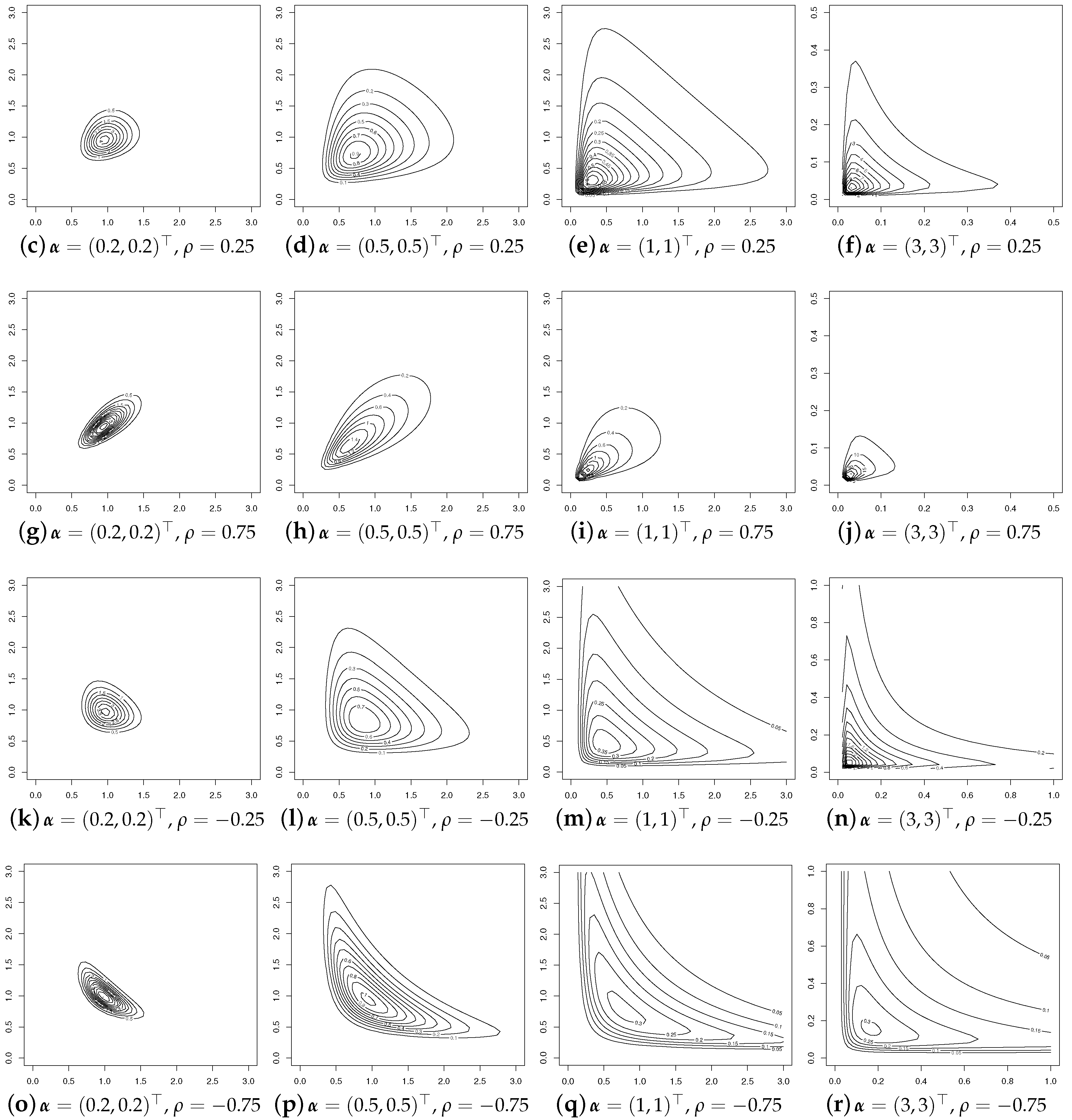
Figure 2 shows contour plots of the BS 2 PDF for ρ { 0.25 , 0.75 , 0.25 , 0.75 } and α = ( α 1 , α 2 ) , with α 1 = α 2 { 0.2 , 0.5 , 1.0 , 3.0 } and λ = ( 1 , 1 ) . Note that the BS 2 distribution is more asymmetric as α 1 and α 2 increase. In addition, it is observed that, as the magnitude of the correlation between the variables increases, the degree of asymmetry in the PDF also increases.
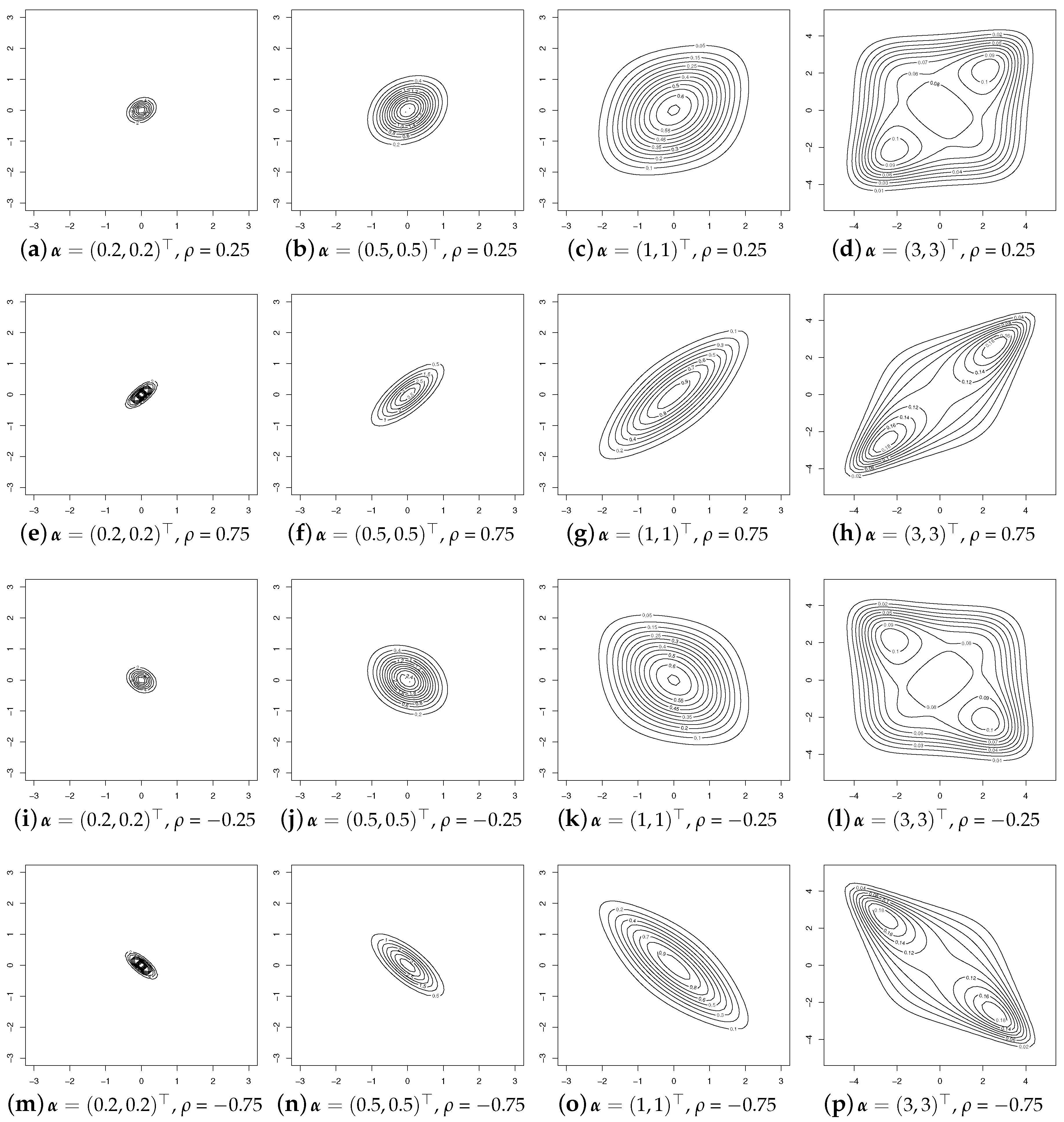
Figure 3 displays contours of the log-BS 2 PDF for ρ { 0.25 , 0.75 , 0.25 , 0.75 } and α = ( α 1 , α 2 ) , with α 1 = α 2 { 0.2 , 0.5 , 1.0 , 3.0 } and μ = ( 0 , 0 ) . Observe that the log-BS 2 distribution is also more asymmetric as α 1 = α 2 increases. Note also that, when α 1 , α 2 > 2 , the log-BS 2 distribution is bimodal, as in the univariate case, but such values are likely to be rare in practice; see Lepadatu et al. (2005); Leiva et al. (2015) and Desousa et al. (2018).

4. Regression Modelling Based on Multivariate Birnbaum–Saunders Distributions

In this section, the regression methodology based on the multivariate BS distribution is presented along with a diagnostic analysis and results from a lifetime modelling example from material science.

4.1. Formulation

The BS log-linear regression model, defined in (8), can be extended to the multivariate case as:
Y = X β + E ,
where Y = ( Y i j ) R n × m is the log-response matrix and X = ( x i s ) R n × p is the model design matrix of rank p, which contains values of p covariates. Here, X , Y are linked by a coefficient matrix β = ( β s j ) = ( β 1 , , β m ) R p × m , and E = ( ε i j ) R n × m is the error matrix. Furthermore, let Y i , x i and ε i be the i-th rows of Y , X and E , respectively. Thus, the model defined in (16) can be rewritten as:
Y i = μ i + ε i = β x i + ε i , i = 1 , , n ,
where ε 1 , , ε n are independently and identically log-BS m ( α 1 m × 1 , 0 m × 1 , Γ ) distributed, with 1 m × 1 being an m × 1 vector of ones.
Consider a sample from a multivariate log-BS distribution, Y = ( Y 1 , , Y n ) , with E [ Y i ] = β x i and observations y = ( y 1 , , y n ) . Then, the log-likelihood function for θ = ( α , vec ( β ) , svec ( Γ ) ) , with ‘vec’ representing the vectorization of a general matrix and ‘svec’ as above, is given by:
( θ ) = m log ( 2 ) m 2 log ( 2 π ) 1 2 log ( | Γ | ) 1 2 ϕ i Γ 1 ϕ i + j = 1 m log ( ξ i j ) ,
where ϕ i = ( ϕ i 1 , , ϕ i m ) , with:
ϕ i j = B ( y i j ; α , μ i j ) = 2 α sinh y i j μ i j 2 , ξ i j = 2 b ( y i j ; α , μ i j ) = 2 α cosh y i j μ i j 2 ,
and μ i j = β j x i , for i = 1 , , n , j = 1 , , m .
The ML estimate θ ^ of θ is defined as the values maximising the log-likelihood function defined in (18). When this corresponds to a stationary point, it can be obtained from the solution of a homogeneous system of equations given by:
( θ ) α = 0 , ( θ ) β * = 0 ( p m ) × 1 , ( θ ) Γ * = 0 ( m ( m 1 ) / 2 ) × 1 ,
where β * = vec ( β ) and Γ * = svec ( Γ ) ; see the details in Marchant et al. (2016). As this system cannot be solved analytically, the ML estimate θ ^ of θ must be found using an iterative procedure. Here, we use the Broyden–Fletcher–Goldfarb–Shanno (BFGS) quasi-Newton procedure (see Lange 2001; Nocedal and Wright 1999) implemented in the R software; see www.R-project.org and R Core Team (2016). In addition, the Hessian matrix is examined to confirm that a valid maximum is obtained.

4.2. Illustration

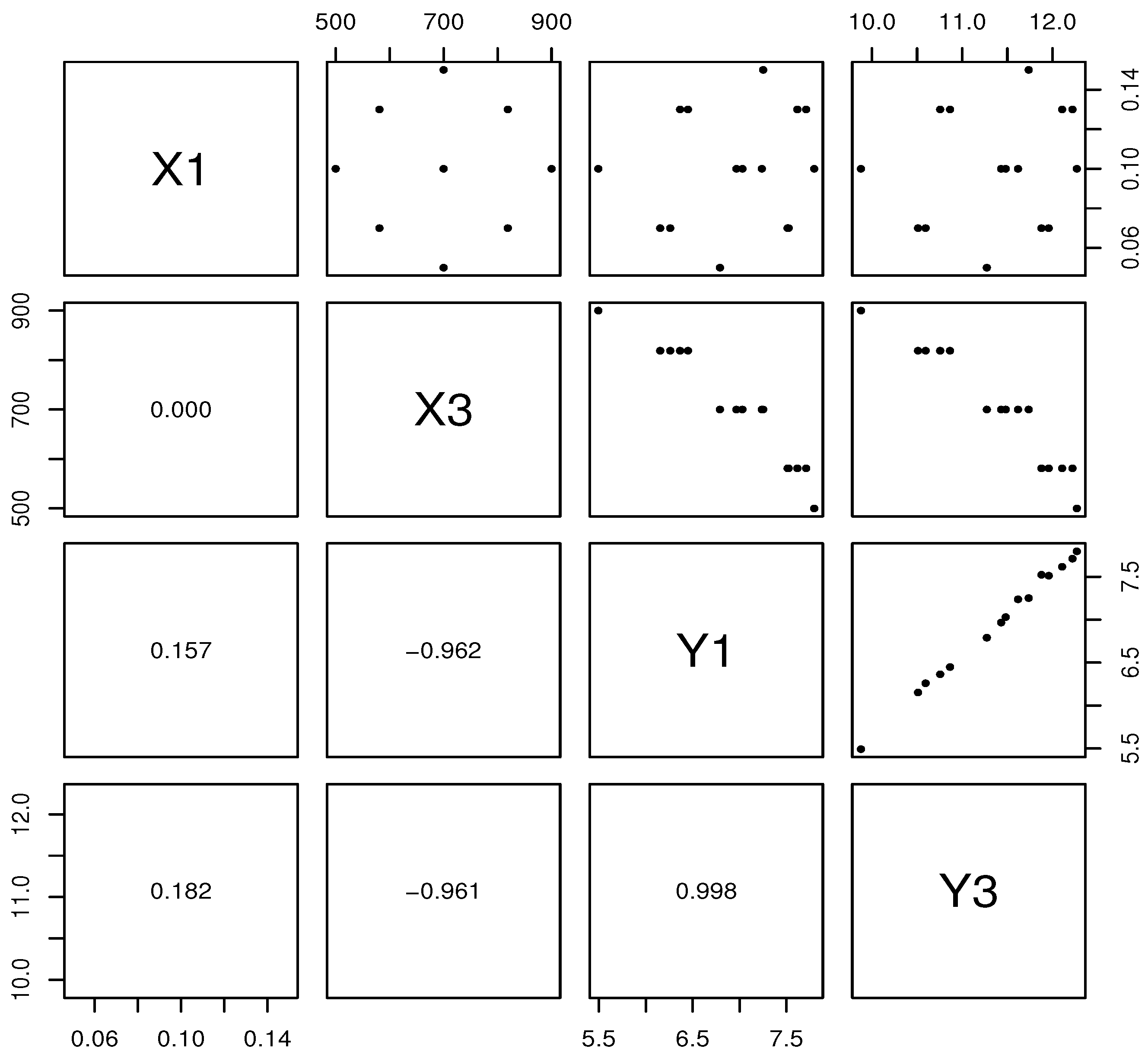
Next, a typical dataset on metal die fatigue in material science is considered, where stress during the regular life cycle of the die eventually leads to failure; see Lepadatu et al. (2005). Although the die lifetime is the main measure of fatigue, other response variables can also be studied. We consider as responses: (i) von Mises stress ( T 1 , in N/mm 2 ) and (ii) manufacturing force ( T 2 , in Newtons (N)); and as covariates: (i) the friction coefficient ( X 1 , dimensionless) and (ii) the working temperature ( X 2 , in °C). Figure 4 shows scatter-plots for log-responses, Y 1 and Y 2 , and covariates, from which we observe that: (i) no correlation exists between ( X 1 , X 2 ) , removing any collinearity concerns; (ii) there is a strong correlation between ( Y 1 , Y 2 ) , justifying the use of a multivariate distribution; (iii) a weak correlation exists between ( X 1 , Y 1 ) and between ( X 1 , Y 2 ) ; and (iv) there is a strong correlation between ( X 2 , Y 1 ) and between ( X 2 , Y 2 ) .
Consider a multivariate BS log-linear regression model to describe ( Y 1 , Y 2 ) as a function of X 2 (since X 1 is omitted due to its weak correlations with the responses). Therefore, the proposed multivariate regression model is given by:
Y i = β x i + ε i , i = 1 , , 15 ,
where ε i = ( ε i 1 , ε i 2 ) log-BS 2 ( α 1 2 × 1 , 0 2 × 1 , Γ ) . ML estimates for the model parameters are shown in Table 1, with corresponding estimated standard errors (SE) and p-values. It can be seen that: (i) the estimated correlation, ρ ^ , is statistically significant at 5%, confirming the conjecture from the exploratory analysis; and (ii) the regression coefficients β 11 , β 12 , β 21 and β 12 must be included in the model.
Validation of the model is based on the MD, after being transformed to normality using the Wilson–Hilferty (WH) approximation; see Ibacache-Pulgar et al. (2014). Probability-probability (PP) plots and acceptance bands associated with the Kolmogorov–Smirnov (KS) statistic for testing normality are constructed using Algorithm 2; for details, see Barros et al. (2014).
Algorithm 2 PP plots with acceptance bands for testing normality.
1:
Consider the data y 1 , , y n , and order them as y 1 : n , , y n : n
2:
Estimate the mean and standard deviation of the normal distribution by y ¯ = j = 1 n y j / n and s y = [ j = 1 n { y ^ j y ¯ } 2 / { n 1 } ] 1 / 2 , respectively. 
3:
Compute o j : n = Φ ( [ y j : n y ¯ ] / s y ) , for j = 1 , , n
4:
Draw the PP plot with points q j : n = [ 2 j 1 ] / [ 2 n ] versus o j : n , for j = 1 , , n
5:
Specify a significance level 1 η
6:
Construct acceptance bands as ( max { q d η + 1 / [ 2 n ] , 0 } , min { q + d η 1 / [ 2 n ] , 1 } ) , where d η is the 100 × η -th percentile of the KS distribution and q is a continuous version of q j : n
7:
Determine the p-value of the KS statistic, and reject the null hypothesis of a normal distribution for the specified significance level based on this p-value. 
8:
Corroborate agreement between Steps 6 and 7.
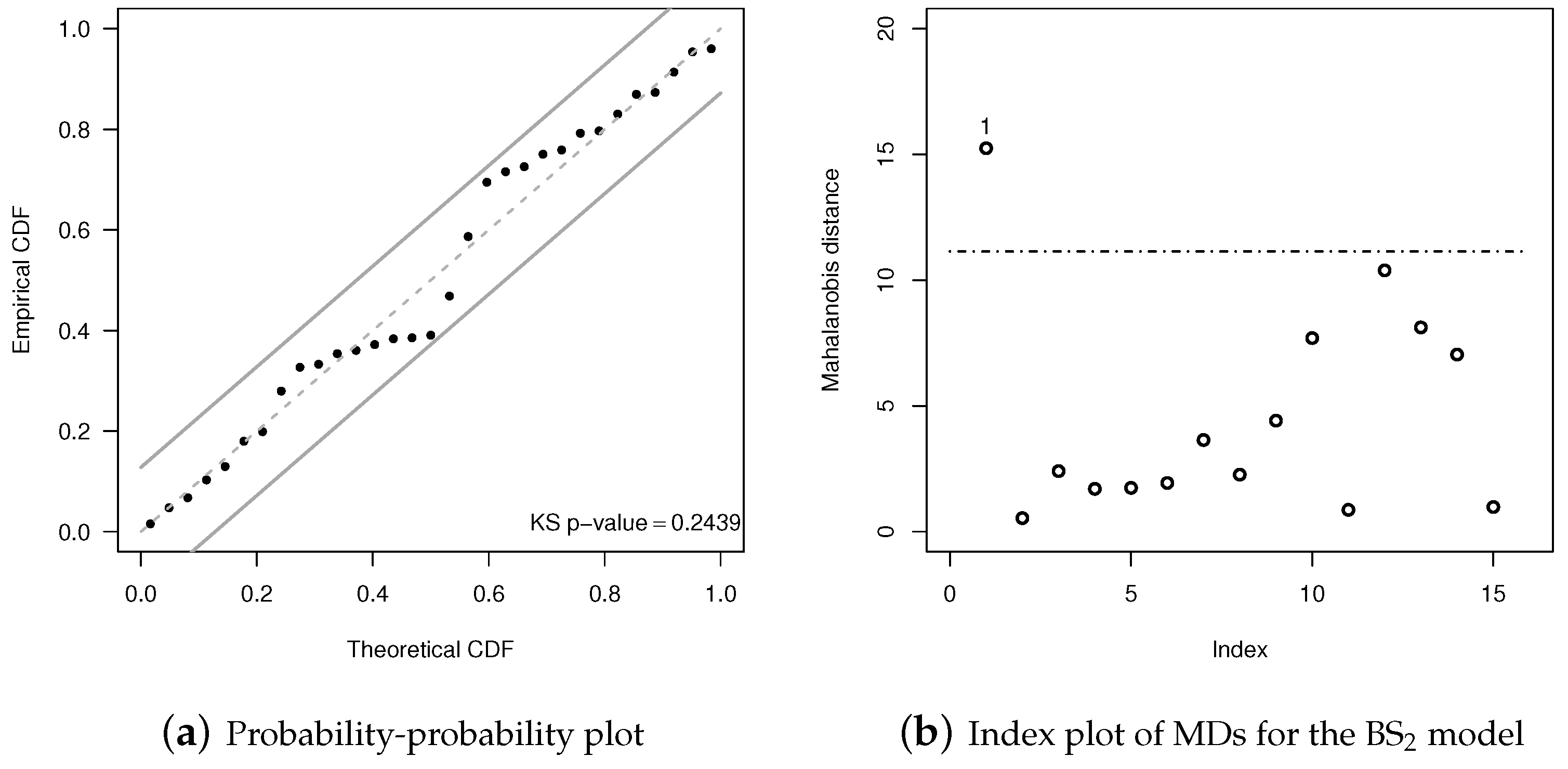
From Figure 5a, which shows the PP plot with acceptance bands for a significance level of 5%, it can be seen that the BS 2 model provides a good fit, which agrees with the p-value of 0.2480 from the associated KS test. Figure 5b displays the MD index plot for the BS 2 log-linear regression model where Observation #1 is identified as a potential multivariate outlier. Figure 6 shows the index plots of total local influence ( C i ) (see Marchant et al. 2016) under the case-weight, correlation, covariate and response perturbation schemes for θ ^ . From this figure, note that Observation #1 has a large influence on the BS 2 log-linear regression model under all perturbation schemes. This observation coincides with that detected by the MD. In addition, Observation #14 seems to have a large influence on the model under case-weight and correlation perturbation schemes. However, when these potentially influential observations are removed, no inferential changes are produced. Therefore, Observations #1 and #14 do not need to be removed, and the prediction model can be estimated considering them.

5. Spatial Modelling Based on Multivariate BS Distributions

In this section, the methodology for estimation and diagnostic analysis using a BS spatial model is presented, along with an example from agricultural engineering.

5.1. Formulation

Consider a stochastic process, { T ( s ) , s D } , defined over region D R 2 . Let T = ( T 1 , , T n ) , where T i = T ( s i ) , for i = 1 , , n , is a collection of n measurements recorded at known locations s = { s 1 , , s n } . Suppose that a suitable spatial model is of the form:
T i = exp ( μ ) η i , i = 1 , , n ,
where η i = η ( s i ) BS ( α , 1 ) , for i = 1 , , n . This assumes that the process is stationary, that is, μ i = μ ( s i ) = μ , and the shape parameter, α , is also assumed to be constant across the spatial locations; see Marchant et al. (2016) and Garcia-Papani et al. (2017). The BS spatial log-linear model is then obtained by taking a logarithmic transformation of (20) to produce:
Y i = log ( T i ) = μ + log ( η i ) = μ + ε i , i = 1 , , n ,
where ε i = log ( η i ) log-BS ( α , 0 ) , for i = 1 , , n . For ease of notation, this is written as:
Y = μ 1 n × 1 + ε ,
where Y = ( Y 1 , , Y n ) R n , ε = ( ε 1 , , ε n ) R n with E ( ε ) = 0 n × 1 and 1 n × 1 as given below (17). Suppose that the covariance between pairs ( Y i , Y j ) is determined by the n × n scale matrix Γ , whose elements can be well described by a Matérn model. This introduces additional parameters φ = ( φ 1 , φ 2 , φ 3 ) ; see details in Garcia-Papani et al. (2017).
Let θ = α , μ , φ 1 , φ 2 , φ 3 be the, just augmented, unknown parameter vector of the model defined in (22). Then, based on the observations y = ( y 1 , , y n ) , the log-likelihood function for θ can be expressed as:
( θ ) = n 2 log ( 2 π ) 1 2 log | Γ | n log ( α ) 2 α 2 V Γ 1 V + i = 1 n log cosh y i μ 2 ,
where V = ( V 1 , , V n ) is an n × 1 vector with elements V i = sinh ( [ y i μ ] / 2 ) , for i = 1 , , n . As in Section 4, we estimate the parameter vector θ with the ML method, but now from the score vector given by:
( θ ) α = 0 , ( θ ) μ = 0 , ( θ ) φ = 0 4 × 1 ;
see the details in Garcia-Papani et al. (2017). As before, there is no analytical solution to this system, and hence, the ML estimate, θ ^ , is again computed using the BFGS iterative procedure.

5.2. Illustration

In this illustration, spatial data from an agricultural study are analysed; for full details, see Garcia-Papani et al. (2017). In the study, the phosphorus content concentration was measured at n = 105 locations over a commercial grain production area of about 170 ha near the town of Cascavel, in the western region of the state of Paraná, Brazil. Phosphorus is an important soil nutrient affecting plant growth, and hence, monitoring its spatial variability is a crucial part of agricultural management. For soy bean, levels are considered low below 3 mg/dm 3 ; medium between about 3 and 6 mg/dm 3 ; high between 6 and 9 mg/dm 3 ; and very high greater than 9 mg/dm 3 . Whereas for corn, the corresponding values are: less than 2 mg/dm 3 , between 2 and 4.5 mg/dm 3 , between 4.6 and 11 mg/dm 3 and greater than 11 mg/dm 3 for low, medium, high and very high, respectively.
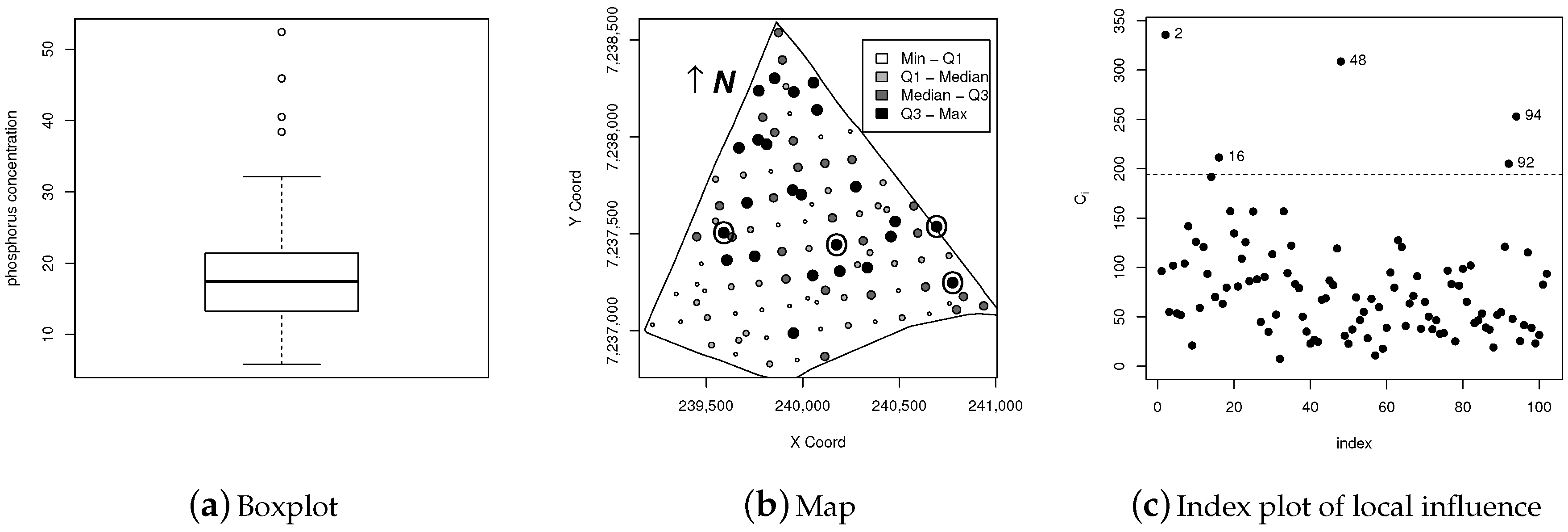
Over the whole study area, the mean phosphorus concentration is 18.11 mg/dm 3 , which is in the very high category for each of the two crops, with coefficients of variation CV = 0.41 (41%), skewness CS = 1.787 and kurtosis CK = 5.104. These indicate a reasonable degree of homogeneity around the mean, a positive skewness and a high kurtosis level, which supports the use of the BS model. Figure 7a shows a boxplot of the data, which identifies Observations #32, #53, #57 and #59 as outliers and contributing to the positive skewness. These values are shown as circled points in Figure 7b, identifying their locations in the lower part of the study area. Examination of directional sample variograms (not displayed here) indicates an isotropic spatial structure, which is described with a Matérn model.
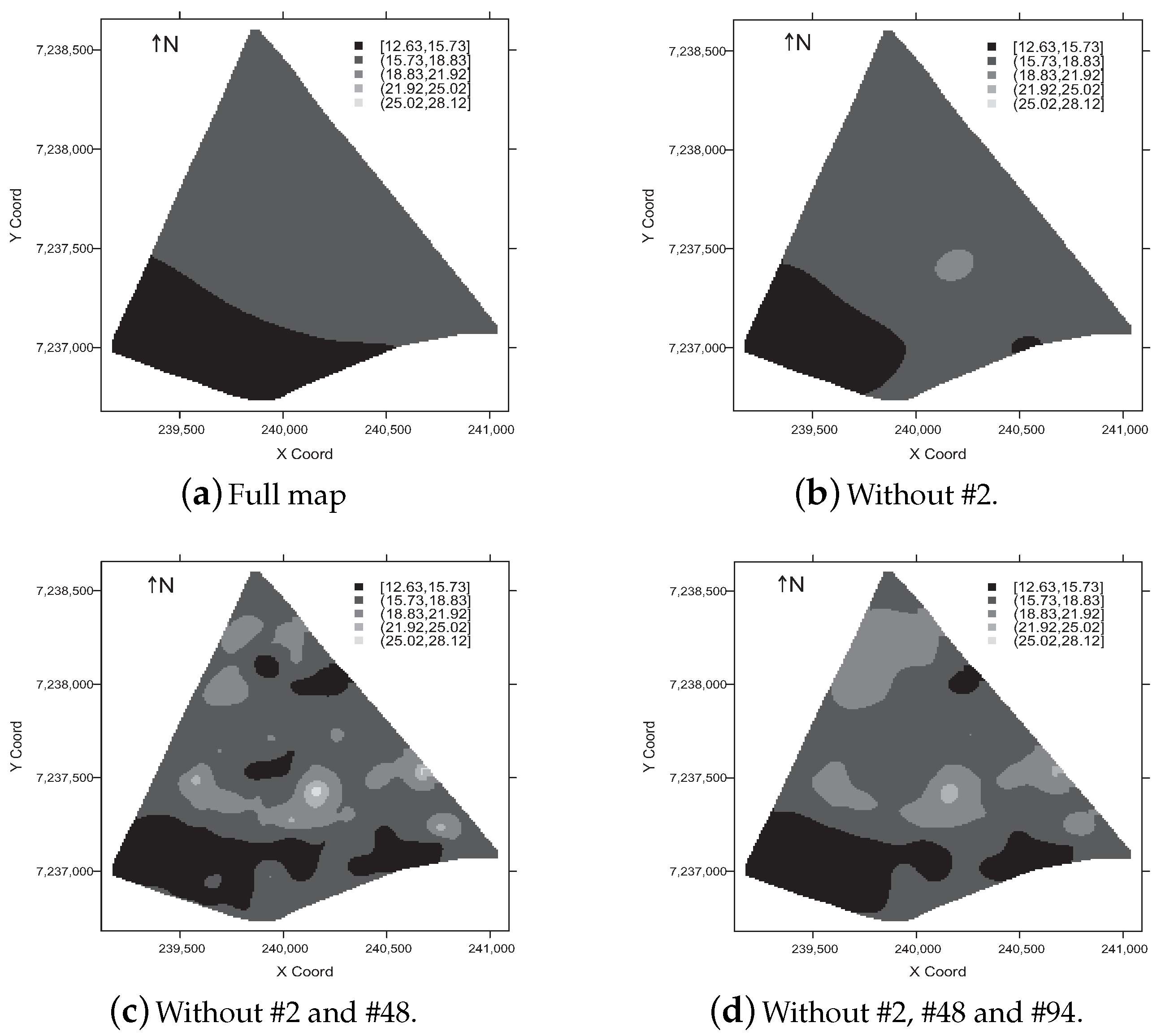
The model parameter, θ , is estimated using the ML method, but the parameter δ , corresponding to the order of the variogram model in the Matérn family, is chosen by cross-validation to avoid identifiability problems in the estimation of the spatial covariance parameters in the Matérn model; see Garcia-Papani et al. (2017). This approach leads to order δ = 2.5 , estimated BS model and variogram parameters (with estimated asymptotic SE in parenthesis) as α ^ = 0.997 ( 3.521 ) , μ ^ = 2.807 ( 0.082 ) , φ ^ 1 = 0.134 ( 0.946 ) , φ ^ 2 = 0.020 ( 0.142 ) , φ ^ 3 = 177.940 ( 0.0000014 ) and a ^ = 1.053 ( 0.0000083 ) ; see Table 2. The fitted scale matrix is then Γ ^ = 0.134 I n + 0.020 R ^ and δ = 2.5 , where I n is the n × n identity matrix; for details of the scale matrix, see Garcia-Papani et al. (2017). Figure 8a shows the resulting fitted spatial map with ordinary kriging interpolation. In all locations, the phosphorus concentration is considered very high and hence is suitable for both crops.
To confirm the suitability of the spatial BS model, it was compared to a Gaussian model using the Akaike information criteria, AIC = 2 ( θ ^ ) + 2 d , and the Bayesian information criteria, BIC = 2 ( θ ^ ) + d log ( n ) , where d is the number of parameters and n the size of the dataset: a smaller value of the information criterion indicates a better model; see Ferreira et al. (2012); Leiva et al. (2015) and the references therein. Numerical values for this example are given in Table 3 showing that the BS model is superior to the Gaussian model. As a further comparison, the Bayes factor (BF), B 12 , allows us to compare two models, denoted by M1 and M2, using 2 log ( B 12 ) BIC M 2 BIC M 1 . An interpretation of the BF, see Table 3, is given in Table 4 leading to the conclusion that the BS model is superior to the Gaussian model with very strong evidence.
Local influence diagnostics are used to assess the effect of the data values on the fitted spatial map shown in Figure 8. Firstly, Figure 7c displays an index plot of C i using the response variable perturbation scheme. This identifies Observations #2, #48 and #94 as potentially influential. Note that the outliers identified by the boxplot in Figure 7a do not include these influential points, which emphasises the importance of using influence methods with preferences for simple univariate outlier detection.
It is now important to see the effects of these three potentially influential points on the parameter estimates and fitted models. Estimated model parameters with corresponding SEs are shown in Table 2 for the full dataset and for subsets with the influential points removed individually and jointly. There are dramatic changes in a ^ , the spatial range parameter, due to corresponding changes in φ ^ 3 since a is a function of φ 3 , and even a change in the Matérn variogram model due to a change in δ . The p-values for hypotheses of the type H 0 : θ j = 0 against H 1 : θ j 0 , where θ j is any of the parameters, are also shown in this table calculated based on the usual asymptotic normal approximation. These identify that μ and φ 3 are significantly different from zero, but that α , φ 1 and φ 2 are not. It is important to also note that removing the potentially influential points has no effect on these inference results.
To visualize the effects of the potentially influential points on the fitted phosphorus concentration maps, consider Figure 8, which uses ordinary kriging interpolation. The map using the full dataset, the reference map, is shown in Figure 8a, with Figure 8b to Figure 8d displaying the maps after removing selected data points. Note that there is a much greater change due to removal of points together rather than individually again, which highlights the importance of considering joint influence. To give a numerical assessment of the changes, two indices have been calculated, the global accuracy (GA) and kappa ( κ ); see Table 2 and the details in Garcia-Papani et al. (2017). Pairs of maps have an acceptable similarity if GA is greater than 0.85, or a low similarity if κ < 0.67 , a medium similarity if 0.67 κ 0.80 and a high similarity if κ > 0.80 ; see Anderson et al. (1976) and Krippendorff (2004). Again, it can be seen that when the potentially influential points are removed separately, the resulting fitted map is similar to the reference map, whereas there is a low similarity when the points are removed together. In particular, removing Observations #2 and #94 leads to a medium similarity, and the others have a low similarity, suggesting that the data points are jointly influential.

6. Multivariate Birnbaum–Saunders Control Charts

In this section, the multivariate log-BS distribution is used in the construction of multivariate control charts, and an application to environmental monitoring is presented. In particular, the parametric bootstrap method (see Hall 2013) is applied to calculate Phase I control limits, and the resulting control chart is used to monitor the process in Phase II.

6.1. Formulation

Suppose that we are interested in modelling a dynamic process with p quality characteristics and that for each there is a sample of n observations from the evolving process. Let  Y i = ( Y i 1 , , Y i p ) R p denote the vector of measured values corresponding to subset i, for  i = 1 , , n . Assume that Y i follows a p-variate log-BS distribution, that is, Y i log-BS p ( α , μ , Γ ) , the vectors Y i are independent over time and μ 0 is the mean vector of the in-control process. To confirm that the process is in control requires testing the hypothesis:
H 0 : μ = μ 0 = ( μ 01 , , μ 0 p ) versus H 1 : μ μ 0 .
This can be achieved using a modified Hotelling T 2 statistic constructed as follows. Using Property (A2) and considering that b i = ( 2 sinh ( [ Y i 1 μ 01 ] / 2 ) , , 2 sinh ( [ Y i p μ 0 p ] / 2 ) has a p-variate normal distribution, that is, b i N p ( 0 p × 1 , D ( α ) Γ D ( α ) ) , for i = 1 , , n , we obtain a Hotelling T 2 statistic adapted for multivariate log-BS distributions as:
T 2 = n ( n 1 ) b ¯ C 1 b ¯ , with b ¯ = i = 1 n b i / n , and C = i = 1 n b i b i .
Note that, if Y log-BS p ( α , μ , Γ ) , then T 2 has a Fisher distribution with degrees of freedom p and n p , that is, T 2 F ( p , n p ) ; see Kundu (2015a). Algorithm 1 can be used to construct the bootstrap distribution of the T 2 statistic using random vectors generated from the p-variate log-BS distribution, and then, Algorithm 3 may be used used to construct the corresponding control limits.
Once constructed, the multivariate BS control chart can be used in Phase II to identify if the evolving process remains in control. Consider a new vector of values of the quality characteristics, and let T new 2 be the corresponding Hotelling statistic calculated using (26). As the process evolves, a sequence of values T new 2 is produced. Algorithm 4 details how to construct p-variate control charts based on BS distributions for process monitoring.
Algorithm 3 Computation of BS control chart limits in Phase I.
1:
Collect k samples ( y 1 h , , y n h ) of size n for an in-control process, with h = 1 , , k , assuming that the p-variate vector with the logarithms of the data follows a log-BS p ( α , μ , Γ ) distribution. 
2:
Compute the ML estimates of α , μ and Γ using the data of the pooled sample of size N = k × n collected in Step 1, and check the distributional assumption using GOF tools. 
3:
Generate a parametric bootstrap sample ( y 1 * , , y n * ) of size n from a p-variate log-GB distribution using the ML estimates obtained in Step 2 as the distribution parameters. 
4:
Compute T 2 defined in (26) with ( y 1 * , , y n * ) , which is denoted by T 2 * , assuming a target μ 0
5:
Repeat Steps 3 to 4 a large number of times (for example, B = 10,000) and obtain B bootstrap statistics of T 2 , denoted by T 1 2 * , , T B 2 *
6:
Fix η as the desired false alarm rate (FAR) of the chart. 
7:
Use the B bootstrap statistics obtained in Step 5 to find the 100 ( η / 2 ) -th and 100 ( 1 η / 2 ) -th quantiles of the distribution of T 2 , which are the lower and upper control limits for the chart of FAR η , respectively.
Algorithm 4 Process monitoring using the multivariate BS chart in Phase II.
1:
Take a sample of size n, namely ( y 1 , , y n ) , from the process. 
2:
Calculate the T new 2 statistic from the sample obtained in Step 1. 
3:
Declare the process as in control if T new 2 falls between lower and upper control limits obtained in Algorithm 3; otherwise, the chart indicates an out-of-control state. 
4:
Repeat Steps 1 to 3 for each sample taken at regular time intervals.

6.2. Illustration

In this illustration, we analyse environmental risk using a multivariate BS quality control chart to monitor urban pollution produced by particulate matter (PM); for further details, see Marchant et al. (2013). The data were collected by the Chilean Metropolitan Environmental Health Service and are available at http://sinca.mma.gob.cl. The data, taken over a calendar year, are hourly averaged concentrations (in μ g/Nm 3 ) of: (i) fine particles of less than 2.5 micrometers, denoted PM2.5 ( X 1 ) and (ii) coarse particles of between 2.5 and 10 micrometers, denoted PM10 ( X 2 ), recorded at 10 monitoring stations from across the metropolitan region of Chile. Here, only the Pudahuel station, near to the city of Santiago, is considered as it is believed to have the worst levels of PM pollution and hence requires careful study. For illustrative purposes, the target values are set at the maximum permitted under Ministry of the Environment guidelines, that is, 50 and 150 μ g/Nm 3 , during 24 h for PM2.5 and PM10, respectively; see CONAMA (1998) and MMA (2011). Figure 9 shows the time series, boxplot and scatter-plot for X 1 and X 2 . From the times series plots, it is clear that the PM2.5 and PM10 concentrations frequently far exceed the target values, and the boxplot indicates substantial positive skewness, suggesting that BS distributions are appropriate, with a large number of potential outliers. In addition, the scatter-plot demonstrates a moderate correlation (0.60) between X 1 and X 2 , which confirms the need to use a multivariate control chart for this dataset.
To construct the control chart in Phase I, data for the first two months are used in Algorithm 3 with k = 59 , n = 24 , N = 1416 , B = 10,000 bootstrap replications and a FAR η = 0.0027 . These months correspond to good and stable air quality representing an in-control process. The modified MD is used with data transformed by the WH approximation to give a normal distribution, and the GOF methods described in Section 4 are used to confirm Step 2 in Algorithm 3. The corresponding PP plots, with KS acceptance regions at 5%, are shown in Figure 10a. These indicate that the BS 2 distribution has a good fit, and this is further supported by the p-value of 0.245 from the corresponding KS test.
In Phase II, the multivariate BS control chart is then used to monitor the air quality for the remaining 10 months of the dataset. This period is partitioned into m = 30 new subgroups each of size n = 24 , giving 720 observations. As illustration, the monitoring of the month of April is provided. Figure 10b shows the PP plot, with 5% acceptance regions, indicating that the BS 2 distribution has a good fit to the data in Phase II, which is again in agreement with the p-value 0.238 from the corresponding KS test. The modified MD index plot in Figure 10c identifies 19 April (labelled as #19) as a multivariate outlier. Figure 10d displays the bivariate BS control chart for monitoring April in Phase II indicating that 10 April (labelled as #10) and 19 April exceed the upper control limit and hence represent an out-of-control state. These would lead to alerts (on the following days) due to dangerous air quality levels with significant risk for human health in the Metropolitan region of Santiago, Chile. This is in agreement with the official information released by the Chilean Ministry of Health, which declared an environmental alert for 11 April; see www.seremisaludrm.cl/sitio/pag/aire/indexjs3airee001.asp.

7. Discussion, Conclusions and Future Research

It has now been 50 years since the birth of the Birnbaum–Saunders distribution, but in that time, it has come a long way. The initial conception was as a model for cumulative damage describing the build-up of fatigue and the eventual failure of materials. As a unimodal distribution and skewed to the right, it found widespread use as a life distribution over a range of applications even outside material science, but initially still based on an argument of cumulative effects. Extensions and generalisations led to multivariate and univariate Birnbaum–Saunders and logarithmic Birnbaum–Saunders distributions, allowing much more varied applications in regression-type modelling. In the last decade, there have also been major advances in goodness of fit assessment and model diagnostics.
In the early development of statistics, methods were linear and usually based on normal distributions. As such, they were tractable for ease of calculation, but lacked flexibility, and hence, appropriate application was constrained. In practice, a wide variety of statistical approaches, built on equally varied distributional foundations, are needed. Each application requires a suitable model. To this end, the Birnbaum–Saunders distribution provides another tool to apply when necessary. In such situations, it has already proven to be sharp, providing reliable and insightful results. The study of Birnbaum–Saunders distributions is now a mature topic, with a substantial literature, which has had significant impact in important and interesting areas. Methods are rigorously defined with theoretical results well understood and developed. We have brought together these theoretical results in a unified and consistent notation to allow greater appreciation of an elegant framework.
There are few uses of Birnbaum–Saunders distributions in the financial and economic sciences, but the potential is substantial. The interpretation of the Birnbaum–Saunders model as an accumulation of incremental damage leading to an abrupt change once a threshold is reached provides a natural description of many financial events. Worldwide financial crises over recent decades have sometimes been attributed to non-normality; for example, the greater downside risk in market movements. In addition, there is a widely acknowledged belief that such processes are skewed and leptokurtic. Through rigorous modelling and the application of appropriate model diagnostics, more robust analyses are possible. This can lead to more accurate understanding of financial processes and more efficient management of products. In particular, a relevant problem in generalized autoregressive conditional heteroskedasticity models is the non-normality of the standardized error distribution, especially the presence of skewness to the right. Although there are several skew distributions to treat this problem, allowing us to capture the skewness and leptokurtosis present in diverse high-frequency financial time series, most of these distributions are focused on the mean. However, when asymmetry is detected, it is well known that the median is a better central tendency indicator than the mean. Then, generalized autoregressive conditional heteroskedasticity type models defined in terms of the median are more suitable than those models based on the mean. The Birnbaum–Saunders distribution has this particular property, putting it ahead of other asymmetric distributions. Some key works that consider this concept related to the autoregressive conditional duration model proposed by Engle and Russell (1998), but based on the Birnbaum–Saunders distribution, are attributed to Bhatti (2010); Leiva et al. (2014) and Saulo et al. (2018). In these works, high-frequency data on financial transactions related to trade duration are studied. Note that the autoregressive conditional duration model is the counterpart of generalized autoregressive conditional heteroskedasticity models for dealing with trade duration data. Therefore, in that context, the Birnbaum–Saunders distributions can capture situations that other asymmetric distributions cannot capture.
Moreover, some distributions can be expressed as a mixture of normal distributions, which may be useful to carry out Bayesian analysis using Monte Carlo Markov chain or variational methods; see, for example, Wand et al. (2011). Some generalizations of the Birnbaum–Saunders distribution can also be represented as a mixture of normal distributions, so that these ideas on Bayesian analysis will be explored in a future work; see Balakrishnan et al. (2009) and Leiva et al. (2014).
In summary, with more sophisticated, yet more appropriate, statistical models, future risks can be more reliably assessed and major financial crises potentially avoided. We have presented new tools for further investigation within this important application area, and we challenge other researchers to start this new exploration in the belief that it can make a worthwhile impact.

Acknowledgments

The research was partially supported by FONDECYT 1160868 project grant from the Chilean Government.

Author Contributions

These authors contributed equally to this article.

Conflicts of Interest

The authors declare no conflict of interest.

References

  1. Alt, Frank. 1985. Multivariate quality control. In The Encyclopedia of Statistical Sciences. Edited by S. Kotz, N. L. Johnson and C. Read. New York: Wiley, pp. 110–12. [Google Scholar]
  2. Anderson, James R., Ernest E. Hardy, John T. Roach, and Richard E. Witmer. 1976. A Land Use and Land Cover Classification System for Use with Remote Sensor Data; Technical Report 964. Washington: US Government Printing Office.
  3. Athayde, Emilia. 2017. A characterization of the Birnbaum–Saunders distribution. REVSTAT Statistical Journal 15: 333–54. [Google Scholar]
  4. Athayde, Emilia, Assis Azevedo, Michelli Barros, and Víctor Leiva. 2018. Failure rate of Birnbaum–Saunders distributions: Shape, change-point, estimation and robustness. Brazilian Journal of Probability and Statistics. in press. [Google Scholar]
  5. Atkinson, Anthony C. 2009. Econometric applications of the forward search in regression: Robustness, diagnostics, and graphics. Econometric Reviews 28: 21–39. [Google Scholar] [CrossRef]
  6. Azevedo, Cecilia, Víctor Leiva, Emilia Athayde, and Narayanaswamy Balakrishnan. 2012. Shape and change point analyses of the Birnbaum–Saunders-t hazard rate and associated estimation. Computational Statistics and Data Analysis 56: 3887–97. [Google Scholar] [CrossRef] [Green Version]
  7. Balakrishnan, Narayanaswamy, Ramesh Gupta, Debasis Kundu, Víctor Leiva, and Antonio Sanhueza. 2011. On some mixture models based on the Birnbaum–Saunders distribution and associated inference. Journal of Statistical Planning and Inference 141: 2175–90. [Google Scholar] [CrossRef]
  8. Balakrishnan, Narayanaswamy, Víctor Leiva, Antonio Sanhueza, and Filidor Vilca. 2009. Estimation in the Birnbaum–Saunders distribution based on scale-mixture of normals and the EM-algorithm. Statistics and Operations Research Transactions 33: 171–92. [Google Scholar]
  9. Barros, Michelli, Víctor Leiva, Raydonal Ospina, and Aline Tsuyuguchi. 2014. Goodness-of-fit tests for the Birnbaum–Saunders distribution with censored reliability data. IEEE Transactions on Reliability 63: 543–54. [Google Scholar] [CrossRef]
  10. Bebbington, Mark, Chin-Diew Lai, and Ricardas Zitikis. 2008. A proof of the shape of the Birnbaum–Saunders hazard rate function. Mathematical Scientist 33: 49–56. [Google Scholar]
  11. Bhatti, Chad. 2010. The Birnbaum–Saunders autoregressive conditional duration model. Mathematics and Computers in Simulation 80: 2062–78. [Google Scholar] [CrossRef]
  12. Birnbaum, Zygmunt W., and Sam C. Saunders. 1969a. A new family of life distributions. Journal of Applied Probability 6: 319–27. [Google Scholar] [CrossRef]
  13. Birnbaum, Zygmunt W., and Sam C. Saunders. 1969b. Estimation for a family of life distributions with applications to fatigue. Journal of Applied Probability 6: 328–47. [Google Scholar] [CrossRef]
  14. Bourguignon, Marcelo, Jeremias Leão, Víctor Leiva, and Manoel Santos-Neto. 2017. The transmuted Birnbaum–Saunders distribution. REVSTAT Statistical Journal 15: 601–28. [Google Scholar]
  15. Caro-Lopera, Francisco, Víctor Leiva, and Narayanaswamy Balakrishnan. 2012. Connection between the Hadamard and matrix products with an application to matrix-variate Birnbaum–Saunders distributions. Journal of Multivariate Analysis 104: 126–39. [Google Scholar] [CrossRef]
  16. Chatterjee, Samprit, and Ali S. Hadi. 1988. Sensitivity Analysis in Linear Regression. New York: Wiley. [Google Scholar]
  17. CONAMA. 1998. Establishment of Primary Quality Guideline for PM10 That Regulates Environmental Alerts; Technical Report Decree 59. Santiago: The Ministry of Environment (CONAMA) of the Chilean Government.
  18. Cook, R. Dennis. 1987. Influence assessment. Journal of Applied Statistics 14: 117–31. [Google Scholar] [CrossRef]
  19. Cook, R. Dennis, and Sanford Weisberg. 1982. Residuals and Influence in Regression. London: Chapman and Hall. [Google Scholar]
  20. D’Agostino, Ralph B., and Michael A. Stephens. 1986. Goodness-of-Fit Techniques. New York: Marcel Dekker. [Google Scholar]
  21. Desmond, Anthony F., Gabriel A. Rodríguez-Yam, and Xuewen Lu. 2008. Estimation of parameters for a Birnbaum–Saunders regression model with censored data. Journal of Statistical Computation and Simulation 78: 983–97. [Google Scholar] [CrossRef]
  22. Desousa, Mario F., Helton Saulo, Víctor Leiva, and Paulo Scalco. 2018. On a tobit-Birnbaum–Saunders model with an application to antibody response to vaccine. Journal of Applied Statistics 45: 932–55. [Google Scholar] [CrossRef]
  23. Dupuis, Debbie J., and Joanna E. Mills. 1998. Robust estimation of the Birnbaum–Saunders distribution. IEEE Transactions on Reliability 1: 88–95. [Google Scholar] [CrossRef]
  24. Engle, Robert, and Jeffrey R. Russell. 1998. Autoregressive conditional duration: A new method for irregularly spaced transaction data. Econometrica 66: 1127–62. [Google Scholar] [CrossRef]
  25. Ferreira, Marta, M. Ivette Gomes, and Víctor Leiva. 2012. On an extreme value version of the Birnbaum–Saunders distribution. REVSTAT Statistical Journal 10: 181–210. [Google Scholar]
  26. Galea, Manuel, Víctor Leiva, and Gilberto A. Paula. 2004. Influence diagnostics in log-Birnbaum–Saunders regression models. Journal of Applied Statistics 31: 1049–64. [Google Scholar] [CrossRef]
  27. Garcia-Papani, Fabiana, Miguel A. Uribe-Opazo, Víctor Leiva, and Robert G. Aykroyd. 2017. Birnbaum-Saunders spatial modelling and diagnostics applied to agricultural engineering data. Stochastic Environmental Research and Risk Assessment 31: 105–24. [Google Scholar] [CrossRef]
  28. Hall, Peter. 2013. The Bootstrap and Edgeworth Expansion. New York: Springer. [Google Scholar]
  29. Hotelling, Harold. 1947. Multivariate Quality Control Illustrated by Air Testing of Sample Bombsights. In Techniques of Statistical Analysis. Edited by C. Eisenhart, M. W. Hastay and W. A. Wallis. New York: McGraw Hill, pp. 111–84. [Google Scholar]
  30. Ibacache-Pulgar, Germán, Gilberto A. Paula, and Manuel Galea. 2014. On influence diagnostics in elliptical multivariate regression models with equicorrelated random errors. Statistical Modelling 16: 14–21. [Google Scholar] [CrossRef]
  31. Jamalizadeh, Ahad, and Debasis Kundu. 2015. Multivariate Birnbaum–Saunders distribution based on multivariate skew-normal distribution. Journal of the Japan Statistical Society 45: 1–20. [Google Scholar] [CrossRef]
  32. Johnson, Norman L., Samuel Kotz, and Narayanaswamy Balakrishnan. 1995. Continuous Univariate Distributions. New York: Wiley, vol. 2. [Google Scholar]
  33. Khosravi, Mohsen, Debasis Kundu, and Ahad Jamalizadeh. 2015. On bivariate and mixture of bivariate Birnbaum-Saunders distributions. Statistical Methodology 23: 1–17. [Google Scholar] [CrossRef]
  34. Kotz, Samuel, Víctor Leiva, and Antonio Sanhueza. 2010. Two new mixture models related to the inverse Gaussian distribution. Methodology and Computing in Applied Probability 12: 199–212. [Google Scholar] [CrossRef]
  35. Krippendorff, Klaus. 2004. Content Analysis: An Introduction to its Methodology. Thousand Oaks: Sage. [Google Scholar]
  36. Kundu, Debasis. 2015a. Bivariate log-Birnbaum-Saunders distribution. Statistics 49: 900–17. [Google Scholar] [CrossRef]
  37. Kundu, Debasis. 2015b. Bivariate sinh-normal distribution and a related model. Brazilian Journal of Probability and Statistics 20: 590–607. [Google Scholar] [CrossRef]
  38. Kundu, Debasis, Narayanaswamy Balakrishnan, and Ahad Jamalizadeh. 2010. Bivariate Birnbaum–Saunders distribution and associated inference. Journal of Multivariate Analysis 101: 113–25. [Google Scholar] [CrossRef]
  39. Kundu, Debasis, Narayanaswamy Balakrishnan, and Ahad Jamalizadeh. 2013. Generalized multivariate Birnbaum–Saunders distributions and related inferential issues. Journal of Multivariate Analysis 116: 230–44. [Google Scholar] [CrossRef]
  40. Kundu, Debasis, N. Kannan, and Narayanaswamy Balakrishnan. 2008. On the hazard function of Birnbaum–Saunders distribution and associated inference. Computational Statistics and Data Analysis 52: 2692–702. [Google Scholar] [CrossRef]
  41. Lange, Kenneth. 2001. Numerical Analysis for Statisticians. New York: Springer. [Google Scholar]
  42. Leão, Jeremias, Víctor Leiva, Helton Saulo, and Vera Tomazella. 2017. Birnbaum–Saunders frailty regression models: Diagnostics and application to medical data. Biometrical Journal 59: 291–314. [Google Scholar] [CrossRef] [PubMed]
  43. Leão, Jeremias, Víctor Leiva, Helton Saulo, and Vera Tomazella. 2018a. A survival model with Birnbaum–Saunders frailty for uncensored and censored cancer data. Brazilian Journal of Probability and Statistics. in press. [Google Scholar]
  44. Leão, Jeremias, Víctor Leiva, Helton Saulo, and Vera Tomazella. 2018b. Incorporation of frailties into a cure rate regression model and its diagnostics and application to melanoma data. Statistics in Medicine. under review. [Google Scholar]
  45. Leiva, Víctor. 2016. The Birnbaum–Saunders Distribution. New York: Academic Press. [Google Scholar]
  46. Leiva, Víctor, Emilia Athayde, Cecilia Azevedo, and Carolina Marchant. 2011. Modeling wind energy flux by a Birnbaum–Saunders distribution with unknown shift parameter. Journal of Applied Statistics 38: 2819–38. [Google Scholar] [CrossRef]
  47. Leiva, Víctor, Marta Ferreira, M. Ivette Gomes, and Camilo Lillo. 2016. Extreme value Birnbaum–Saunders regression models applied to environmental data. Stochastic Environmental Research and Risk Assessment 30: 1045–58. [Google Scholar] [CrossRef]
  48. Leiva, Víctor, Carolina Marchant, Fabrizio Ruggeri, and Helton Saulo. 2015. A criterion for environmental assessment using Birnbaum–Saunders attribute control charts. Environmetrics 26: 463–76. [Google Scholar] [CrossRef]
  49. Leiva, Víctor, Carolina Marchant, Helton Saulo, Muhammad Aslam, and Fernando Rojas. 2014. Capability indices for Birnbaum–Saunders processes applied to electronic and food industries. Journal of Applied Statistics 41: 1881–902. [Google Scholar] [CrossRef]
  50. Leiva, Víctor, M. Guadalupe Ponce, Carolina Marchant, and Oscar Bustos. 2012. Fatigue statistical distributions useful for modeling diameter and mortality of trees. Revista Colombiana de Estadística 35: 349–67. [Google Scholar]
  51. Leiva, Víctor, Edgardo Rojas, Manuel Galea, and Antonio Sanhueza. 2014. Diagnostics in Birnbaum–Saunders accelerated life models with an application to fatigue data. Applied Stochastic Models in Business and Industry 30: 115–31. [Google Scholar] [CrossRef]
  52. Leiva, Víctor, Fabrizio Ruggeri, Helton Saulo, and Juan F. Vivanco. 2017. A methodology based on the Birnbaum–Saunders distribution for reliability analysis applied to nano-materials. Reliability Engineering and System Safety 157: 192–201. [Google Scholar] [CrossRef]
  53. Leiva, Víctor, Antonio Sanhueza, and José M. Angulo. 2009. A length-biased version of the Birnbaum–Saunders distribution with application in water quality. Stochastic Environmental Research and Risk Assessment 23: 299–307. [Google Scholar] [CrossRef]
  54. Leiva, Víctor, Antonio Sanhueza, Samuel Kotz, and Nelson Araneda. 2010. A unified mixture model based on the inverse Gaussian distribution. Pakistan Journal of Statistics 26: 445–60. [Google Scholar]
  55. Leiva, Víctor, Antonio Sanhueza, Pranab K. Sen, and Gilberto A. Paula. 2008. Random number generators for the generalized Birnbaum–Saunders distribution. Journal of Statistical Computation and Simulation 78: 1105–18. [Google Scholar] [CrossRef]
  56. Leiva, Víctor, Manoel Santos-Neto, Francisco José A. Cysneiros, and Michelli Barros. 2014. Birnbaum–Saunders statistical modelling: A new approach. Statistical Modelling 14: 21–48. [Google Scholar] [CrossRef]
  57. Leiva, Víctor, Manoel Santos-Neto, Francisco José A. Cysneiros, and Michelli Barros. 2016. A methodology for stochastic inventory models based on a zero-adjusted Birnbaum–Saunders distribution. Applied Stochastic Models in Business and Industry 32: 74–89. [Google Scholar] [CrossRef]
  58. Leiva, Víctor, and Helton Saulo. 2017. Environmental applications based on Birnbaum–Saunders models. In Mathematical and Statistical Applications in Life Sciences and Engineering. Edited by A. Adhikari, M. Adhikari and Y. Chaubey. New York: Springer, pp. 283–304. [Google Scholar]
  59. Leiva, Víctor, Helton Saulo, Jeremias Leão, and Carolina Marchant. 2014. A family of autoregressive conditional duration models applied to financial data. Computational Statistics and Data Analysis 79: 175–91. [Google Scholar] [CrossRef]
  60. Leiva, Víctor, and Sam C. Saunders. 2015. Cumulative damage models. Wiley StatsRef: Statistics Reference Online 1: 1–10. [Google Scholar]
  61. Leiva, Víctor, Mauricio Tejo, Pierre Guiraud, Oliver Schmachtenberg, Patricio Orio, and Fernando Marmolejo-Ramos. 2015. Modeling neural activity with cumulative damage distributions. Biological Cybernetics 109: 421–33. [Google Scholar] [CrossRef] [PubMed]
  62. Leiva, Víctor, and Juan F. Vivanco. 2016. Fatigue models. Wiley StatsRef: Statistics Reference Online 1: 1–10. [Google Scholar]
  63. Lemonte, Artur J. 2011. Covariance matrix formula for Birnbaum–Saunders regression models. Journal of Statistical Computation and Simulation 81: 899–908. [Google Scholar] [CrossRef]
  64. Lemonte, Artur J., and Silvia L. P. Ferrari. 2011a. Signed likelihood ratio tests in the Birnbaum–Saunders regression model. Journal of Statistical Planning and Inference 141: 1031–40. [Google Scholar] [CrossRef]
  65. Lemonte, Artur J., and Silvia L. P. Ferrari. 2011b. Small-sample corrections for score tests in Birnbaum–Saunders regressions. Communications in Statistics: Theory and Methods 40: 232–43. [Google Scholar] [CrossRef]
  66. Lemonte, Artur J., Guillermo Martínez-Flores, and Germán Moreno-Arenas. 2015. Multivariate Birnbaum–Saunders distribution: Properties and associated inference. Journal of Statistical Computation and Simulation 85: 374–92. [Google Scholar] [CrossRef]
  67. Lemonte, Artur J., Alexandre Simas, and Francisco Cribari-Neto. 2008. Bootstrap-based improved estimators for the two-parameter Birnbaum–Saunders distribution. Journal of Statistical Computation and Simulation 78: 37–49. [Google Scholar] [CrossRef]
  68. Lemonte, Artur J. 2016. Robust inference for Birnbaum–Saunders regressions. Journal of Statistical Computation and Simulation 86: 611–22. [Google Scholar] [CrossRef]
  69. Lepadatu, Daniel, Abdessamad Kobi, Ridha Hambli, and Alain Barreau. 2005. Lifetime multiple response optimization of metal extrusion die. Proceedings of the Annual Reliability and Maintainability Symposium, Institute of Electrical and Electronics Engineers 1: 37–42. [Google Scholar]
  70. Lillo, Camilo, Víctor Leiva, Orietta Nicolis, and Robert G. Aykroyd. 2018. L-moments of the Birnbaum–Saunders distribution and its extreme value version: Estimation, goodness of fit and application to earthquake data. Journal of Applied Statistics 45: 187–209. [Google Scholar] [CrossRef]
  71. Lio, Yuhlong L., and Chanseok Park. 2008. A bootstrap control chart for Birnbaum–Saunders percentiles. Quality and Reliability Engineering International 24: 585–600. [Google Scholar] [CrossRef]
  72. Marchant, Carolina, Víctor Leiva, M. Fernanda Cavieres, and Antonio Sanhueza. 2013. Air contaminant statistical distributions with application to PM10 in Santiago, Chile. Reviews of Environmental Contamination and Toxicology 223: 1–31. [Google Scholar] [PubMed]
  73. Marchant, Carolina, Víctor Leiva, and Francisco José A. Cysneiros. 2016. A multivariate log-linear model for Birnbaum–Saunders distributions. IEEE Transactions on Reliability 65: 816–27. [Google Scholar] [CrossRef]
  74. Marchant, Carolina, Víctor Leiva, Francisco José A. Cysneiros, and Shuangzhe Liu. 2018. Robust multivariate control charts based on Birnbaum–Saunders distributions. Journal of Statistical Computation and Simulation 88: 182–202. [Google Scholar] [CrossRef]
  75. Marchant, Carolina, Víctor Leiva, Franciso José A. Cysneiros, and Juan F. Vivanco. 2016. Diagnostics in multivariate generalized Birnbaum–Saunders regression models. Journal of Applied Statistics 43: 2829–49. [Google Scholar] [CrossRef]
  76. MMA. 2011. Establishment of Primary Quality Guideline for Inhalable Fine Particulate Matter PM2.5; Technical Report Decree 12. Santiago: The Ministry of Environment of the Chilean Government.
  77. Nocedal, Jorge, and Stephen J. Wright. 1999. Numerical Optimization. New York: Springer. [Google Scholar]
  78. Osorio, Felipe, Gilberto A. Paula, and Manuel Galea. 2007. Assessment of local influence in elliptical linear models with longitudinal structure. Computational Statistics and Data Analysis 51: 4354–68. [Google Scholar] [CrossRef]
  79. Owen, William J. 2006. A new three-parameter extension to the Birnbaum–Saunders distribution. IEEE Transactions on Reliability 55: 475–79. [Google Scholar] [CrossRef]
  80. Owen, William J., and William J. Padgett. 1999. Accelerated test models for system strength based on Birnbaum–Saunders distribution. Lifetime Data Analysis 5: 133–47. [Google Scholar] [CrossRef] [PubMed]
  81. Owen, William J., and William J. Padgett. 2000. A Birnbaum–Saunderss accelerated life model. IEEE Transactions on Reliability 49: 224–29. [Google Scholar] [CrossRef]
  82. Paula, Gilberto A. 1993. Assessing local influence in restricted regression models. Communications in Statistics: Theory and Methods 16: 63–79. [Google Scholar] [CrossRef]
  83. Paula, Gilberto A., Víctor Leiva, Michelli Barros, and Shuangzhe Liu. 2012. Robust statistical modeling using the Birnbaum–Saunders-t distribution applied to insurance. Applied Stochastic Models in Business and Industry 28: 16–34. [Google Scholar] [CrossRef]
  84. R Core Team. 2016. R: A Language and Environment for Statistical Computing. Vienna: R Foundation for Statistical Computing. [Google Scholar]
  85. Rieck, James R. 2003. A comparison of two random number generators for the Birnbaum–Saunders distribution. Communications in Statistics: Theory and Methods 32: 929–34. [Google Scholar] [CrossRef]
  86. Rieck, James R., and Jerry R. Nedelman. 1991. A log-linear model for the Birnbaum–Saunders distribution. Technometrics 3: 51–60. [Google Scholar]
  87. Rojas, Fernando, Víctor Leiva, Peter Wanke, and Carolina Marchant. 2015. Optimization of contribution margins in food services by modeling independent component demand. Revista Colombiana de Estadística 38: 1–30. [Google Scholar] [CrossRef]
  88. Sánchez, Luis, Víctor Leiva, Francisco J. Caro-Lopera, and Franciso José A. Cysneiros. 2015. On matrix-variate Birnbaum-Saunders distributions and their estimation and application. Brazilian Journal of Probability and Statistics 29: 790–812. [Google Scholar] [CrossRef]
  89. Santana, Lucia, Filidor Vilca, and Víctor Leiva. 2011. Influence analysis in skew-Birnbaum–Saunders regression models and applications. Journal of Applied Statistics 38: 1633–49. [Google Scholar] [CrossRef]
  90. Santos-Neto, Manoel, Franciso José A. Cysneiros, Víctor Leiva, and S. Ejaz Ahmed. 2012. On new parameterizations of the Birnbaum–Saunders distribution. Pakistan Journal of Statistics 28: 1–26. [Google Scholar]
  91. Santos-Neto, Manoel, Franciso José A. Cysneiros, Víctor Leiva, and Michelli Barros. 2014. On new parameterizations of the Birnbaum–Saunders distribution and its moments, estimation and application. REVSTAT Statistical Journal 12: 247–72. [Google Scholar]
  92. Santos-Neto, Manoel, Franciso José A. Cysneiros, Víctor Leiva, and Michelli Barros. 2016. Reparameterized Birnbaum–Saunders regression models with varying precision. Electronic Journal of Statistics 10: 2825–55. [Google Scholar] [CrossRef]
  93. Saulo, Helton, J. Leão, Víctor Leiva, and Robert G. Aykroyd. 2018. Birnbaum-Saunders autoregressive conditional duration models applied to high-frequency financial data. Statistical Papers, 1–25. [Google Scholar] [CrossRef]
  94. Saulo, Helton, Víctor Leiva, Flavio A. Ziegelmann, and Carolina Marchant. 2013. A nonparametric method for estimating asymmetric densities based on skewed Birnbaum–Saunders distributions applied to environmental data. Stochastic Environmental Research and Risk Assessment 27: 1479–91. [Google Scholar] [CrossRef]
  95. Shewhart, Walter A. 1931. Economic Control of Quality of Manufactured Product. New York: D. Van Nostrand Company. [Google Scholar]
  96. Shi, Lei. 1997. Local influence in principal components analysis. Biometrika 84: 175–86. [Google Scholar] [CrossRef]
  97. Tsionas, Efthymios G. 2001. Bayesian inference in Birnbaum–Saunders regression. Communications in Statistics: Theory and Methods 30: 179–93. [Google Scholar] [CrossRef]
  98. Vilca, Filidor, Narayanaswamy Balakrishnan, and Camila Borelli Zeller. 2014. A robust extension of the bivariate Birnbaum–Saunders distribution and associated inference. Journal of Multivariate Analysis 124: 418–35. [Google Scholar] [CrossRef]
  99. Vilca, Filidor, Antonio Sanhueza, Víctor Leiva, and George Christakos. 2010. An extended Birnbaum–Saunders model and its application in the study of environmental quality in Santiago, Chile. Stochastic Environmental Research and Risk Assessment 24: 771–82. [Google Scholar] [CrossRef]
  100. Villegas, Cristian, Gilberto A. Paula, and Víctor Leiva. 2011. Birnbaum–Saunders mixed models for censored reliability data analysis. IEEE Transactions on Reliability 60: 748–58. [Google Scholar] [CrossRef]
  101. Volodin, Igor N., and Olga A. Dzhungurova. 2000. On limit distribution emerging in the generalized Birnbaum–Saunders model. Journal of Mathematical Science 99: 1348–66. [Google Scholar] [CrossRef]
  102. Wand, Matt P., John T. Ormerod, Simone A. Padoan, and Rudi Frühwirth. 2011. Mean field variational Bayes for elaborate distributions. Bayesian Analysis 6: 847–900. [Google Scholar] [CrossRef]
  103. Wang, Min, Chanseok Park, and Xiaoqian Sun. 2015. Simple robust parameter estimation for the Birnbaum–Saunders distribution. Journal of Statistical Distributions and Applications 2: 1–11. [Google Scholar] [CrossRef]
  104. Wang, Min, Jng Zhao, Xiaoqian Sun, and Chanseok Park. 2013. Robust explicit estimation of the two-parameter Birnbaum–Saunders distribution. Journal of Applied Statistics 40: 2259–74. [Google Scholar] [CrossRef]
  105. Wanke, Peter, and Víctor Leiva. 2015. Exploring the potential use of the Birnbaum–Saunders distribution in inventory management. Mathematical Problems in Engineering 2015: 827246. [Google Scholar] [CrossRef]
  106. Xia, Jianhong, Panlop Zeephongsekul, and David Packer. 2011. Spatial and temporal modelling of tourist movements using semi-Markov processes. Tourism Management 51: 844–51. [Google Scholar] [CrossRef]
  107. Xie, Feng-Chang, and Cheng Wei. 2007. Diagnostics analysis for log-Birnbaum–Saunders regression models. Computational Statistics and Data Analysis 51: 4692–96. [Google Scholar] [CrossRef]
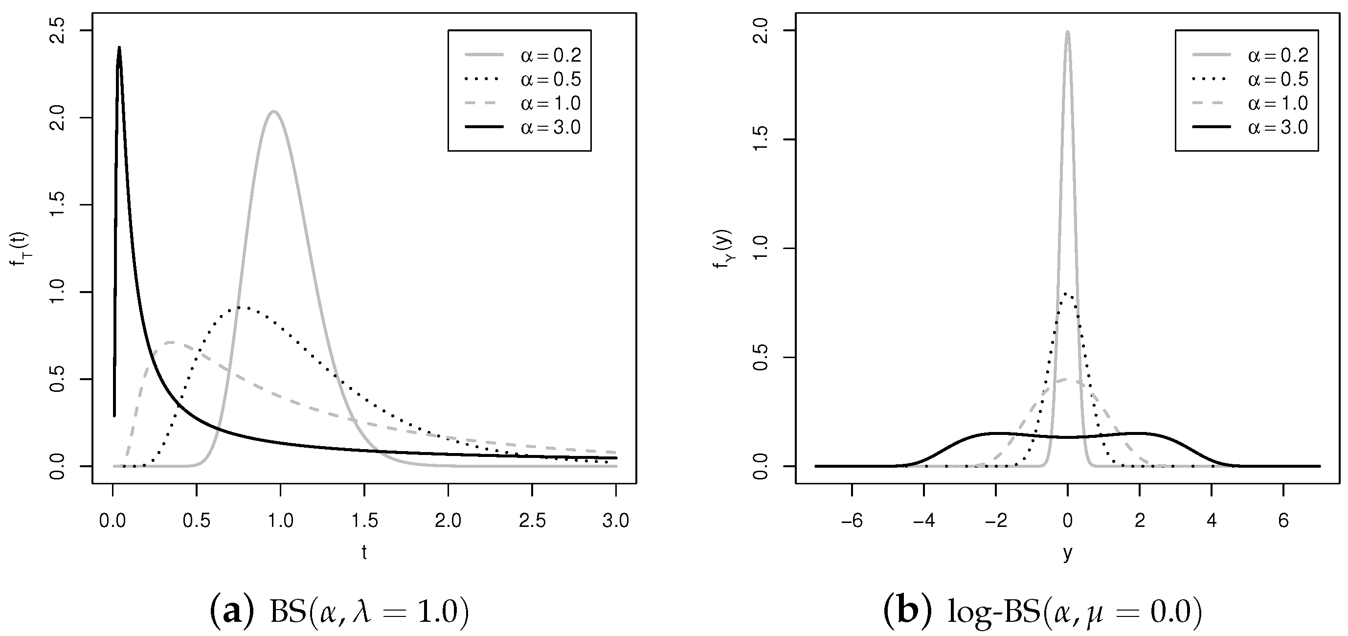
Figure 1. Probability density functions of Birnbaum–Saunders (BS) and log-BS distributions for the indicated α .
Risks 06 00021 g001
Figure 2. Contour plots for the BS 2 distribution with λ = ( 1 , 1 ) and indicated α = ( α 1 , α 2 ) , ρ .
Risks 06 00021 g002
Figure 3. Contour plots for the log-BS 2 distribution with μ = ( 0 , 0 ) and indicated α = ( α 1 , α 2 ) , ρ .
Risks 06 00021 g003
Figure 4. Scatter-plots of the die fracture data variables along with corresponding correlations.
Risks 06 00021 g004
Figure 5. (a) Probability-probability (PP) plot with KS acceptance region at 5% for transformed Mahalanobis distances (MDs) with the BS 2 model and (b) an index plot of MDs for the BS 2 model and indicated perturbation scheme with die lifetime data.
Risks 06 00021 g005
Figure 6. Index plots of total local influence for θ ^ with die lifetime data.
Risks 06 00021 g006
Figure 7. Results for phosphorus concentration data.
Risks 06 00021 g007
Figure 8. Contour plots showing the effects of removing the indicated observation(s) for phosphorus data.
Risks 06 00021 g008
Figure 9. Data summaries for X 1 and X 2 at the Pudahuel monitoring station.
Risks 06 00021 g009
Figure 10. PP plots with 5% KS acceptance regions for the modified MD using the BS 2 distribution in (a) Phase I and (b) Phase II, then (c) the MD index plot and (d) the BS control chart based on PM data.
Risks 06 00021 g010
Table 1. Maximum likelihood (ML) estimate of the indicated parameter with corresponding estimated asymptotic standard errors and p-values of the usual normal approximation hypothesis test using die lifetime data.
Parameter
α β 11 β 12 β 21 β 22 ρ
ML estimate0.14740710.89798115.524423−0.005647−0.0059300.972392
Standard error0.0148130.2361750.2358650.0003330.0003330.005219
p-value<0.001<0.001<0.001<0.001<0.001<0.001
Table 2. ML parameter estimates with SE in parenthesis and p-values in brackets, as well as the values of global accuracy (GA) and κ indices for the phosphorus concentration dataset with indicated case(s) removed.
Removed case(s)Matérn Order α ^ μ ^ φ 1 ^ φ 2 ^ φ 3 ^ a ^ GA κ
0.9972.8070.1340.020177.9401053.405--
None δ = 2.5 (3.521)(0.082)(0.946)(0.142)(0.0000014)(0.0000083)
[0.389][<0.001][0.444][0.444][<0.001][<0.001]
0.9932.8310.1250.016108.655643.2380.900.72
#2 δ = 2.5 (4.097)(0.059)(1.031)(0.132)(0.0000008)(0.0000047)
[0.404][<0.001][0.452][0.452][<0.001][<0.001]
0.9962.8240.1250.019152.374902.0540.970.92
#48 δ = 2.5 (3.417)(0.073)(0.856)(0.133)(0.0000012)(0.0000071)
[0.386][<0.001][0.442][0.443][<0.001][<0.001]
0.9972.8170.1220.028308.8281235.3120.840.69
#94 δ = 1 (3.417)(0.073)(0.856)(0.133)(0.0000012)(0.0009092)
[0.374][<0.001][0.436][0.437][<0.001][<0.001]
0.9912.8450.0710.06081.052243.1560.650.31
#2, #48 δ = 0.5
(exponential)
(6.149)(0.046)(0.882)(0.746)(0.0000884)(0.0002652)
[0.436][<0.001][0.468][0.469][<0.001][<0.001]
0.9952.8400.0970.038182.059546.1770.720.45
#2, #94 δ = 0.5
(exponential)
(3.308)(0.063)(0.644)(0.254)(0.0002974)(0.0008922)
[0.382][<0.001][0.440][0.441][<0.001][<0.001]
0.9942.8340.1140.024144.768856.7370.800.60
#48, #94 δ = 2.5 (2.980)(0.077)(0.683)(0.145)(0.0000010)(0.0000059)
[0.370][<0.001][0.434][0.435][<0.001][<0.001]
0.9822.8550.0850.041143.699431.0970.660.35
#2, #48, #94 δ = 0.5
(exponential)
(3.442)(0.056)(0.597)(0.287)(0.0002051)(0.0006153)
[0.388][<0.001][0.444][0.443][<0.001][<0.001]
Table 3. Analysis of the phosphorus concentration data; log-likelihood, Akaike information criteria (AIC), Bayesian information criteria (BIC) and 2 log ( B 12 ) for the Birnbaum-Saunders (BS) and Gaussian models.
Model ( θ ^ ) AICBIC 2 log ( B 12 )
BS 332.576 675.152 688.276 28.224
Gaussian 349.000 706.000 716.500
Table 4. Interpretation of 2 log ( B 12 ) associated with the Bayes factor (BF).
2 log ( B 12 ) Evidence in Favour of M 1
<0Negative ( M 2 is accepted)
[ 0 , 2 ) Weak
[ 2 , 6 ) Positive
[ 6 , 10 ) Strong
≥10Very strong