Article

Backtesting the Lee–Carter and the Cairns–Blake–Dowd Stochastic Mortality Models on Italian Death Rates

by
Carlo Maccheroni
1,2,* and
Samuel Nocito
2,*
1
Dondena Centre for Research on Social Dynamics, Bocconi University, 20100 Milano, Italy
2
University of Turin, 10124 Torino, Italy
*
Authors to whom correspondence should be addressed.
Risks 2017, 5(3), 34; https://doi.org/10.3390/risks5030034
Submission received: 23 December 2016 / Revised: 21 June 2017 / Accepted: 27 June 2017 / Published: 4 July 2017

Abstract

:
This work proposes a backtesting analysis that compares the Lee–Carter and the Cairns–Blake–Dowd mortality models, employing Italian data. The mortality data come from the Italian National Statistics Institute (ISTAT) database and span the period 1975–2014, over which we computed back-projections evaluating the performances of the models compared with real data. We propose three different backtest approaches, evaluating the goodness of short-run forecast versus medium-length ones. We find that neither model was able to capture the improving shock on mortality observed for the male population on the analysed period. Moreover, the results suggest that CBD forecasts are reliable prevalently for ages above 75, and that LC forecasts are basically more accurate for this data.

1. Introduction

Dowd et al. (2010a) performed a backtesting analysis on seven different stochastic mortality models with results showing that the models performed adequately by most backtests. The analysis was applied to English and Welsh male mortality data. We decided to perform a backtesting investigation using Italian mortality data. The decision was motivated by the study of the historical mortality trend, observed on the forty-past-years horizon for both the male and female populations. The gap between genders deeply decreased over the considered horizon with steep improvements in male mortality. Thus, the first aim of this paper is to scrutinize the forecast proposed by the models for both sexes, which have experienced different mortality evolutions. Moreover, in the last three decades, mortality projections have been widely used by Italian policy-makers for making decisions about public pension reforms. The study of mortality risk, intended as the uncertainty in future mortality rates as well as longevity risk for the long-term trend in mortality rates (Cairns et al. 2006), played a central role for both public and private annuity providers. For these reasons, among all the principal stochastic mortality models1, we chose to compare Lee–Carter (LC) and the Cairns–Blake–Dowd (CBD) ones. In particular, the Italian National Statistics Institute (ISTAT) adopted the original formulation of the LC model to forecast mortality over the projection horizon 2007–2051 (Istat 2008) now updated2 over the horizon 2011–2065. The National Association of Insurance Companies (ANIA) uses those projections as demographic basis for annuity computations (ANIA 2014). Therefore, we chose to compare the original formulation of the LC model to the original CBD since they also represent the two most used parametric families of mortality models.
On the one hand, the Lee–Carter model has sparked a deep methodological revolution in the field of demographic forecast, particularly in mortality. The mortality model has been used together with a similar fertility model and deterministic migration assumptions to generate stochastic forecasts about the population and its components. These stochastic population forecasts, in turn, have been used as the key component of stochastic projections of the finances of the US Social Security system. The stochastic forecast avoids some of the problems inherent to using the classic scenario method for representing forecast uncertainty (Lee 2000). Then, in concurrence with the main demographic applications, the LC model suggested:
On the other hand, the Cairns–Blake–Dowd model, even if more recent in its formulation than the LC model, has played an important role in forecasting mortality at higher ages (i.e., ages starting at 60 and over). The mortality model made great contributions for pension funds, life-insurance companies and private annuity providers in general. It is mainly used for pricing longevity bonds as suggested also by the authors in the first formulation of the model (Cairns et al. 2006).
The second aim of this work is to analyse the medium-length forecast with respect to the short term, observing potential differences in the parameter estimations (Mavros et al. 2014)3 accordingly with changes in the starting point of the database. Chan et al. (2014) have also studied the new-data-invariant property on the quality of the CBD mortality index. For this purpose, we introduced a new backtesting approach named the jumping fixed-length horizon, which makes short-run projections of five years, “jumping forward” in the historical database by five-year-steps.
Considerations of the backtesting results do not imply a conclusive evaluation of the models, since we perform the analysis exclusively for the range of ages 57 to 90. The choice for the interval of ages was motivated by the fact that, in Italy, Ragioneria dello Stato computes the so-called transformation coefficients for pension annuities, starting from age 57. Moreover, since the CBD model is recommended as a good predictor of mortality at higher ages, we chose this interval of ages to make a more prudent and accurate comparison between the models. Furthermore, we decided to take into consideration only death probabilities q x , t among all of the other possible biometric functions.
We used4 death probabilities q x , t provided by ISTAT spanning the period 1975–2014. Then, over the designated horizon of historical data, we select the “lookback” and the “lookforward” windows5, respectively, for the parameter estimation and forecast. In particular, the length of the forecast window will be different for each of the three backtesting approaches proposed by the work:
  • fixed horizon backtests: lookback and lookforward windows of 20 years;
  • jumping fixed-length horizon backtests: lookback window of 20 years and lookforward window of 5 years (short-term projections); and
  • rolling fixed-length horizon backtests: lookback window of fixed-length (20 years) and a contracting lookforward window from 20 to 2 years of projections.
The paper is organized as follows. Section 2 briefly presents the models and the adopted terminology, Section 3 shows the historical Italian mortality data, and Section 4 and subsections explain methodology and the backtesting results obtained by the different approaches. Section 5 provides conclusions.

2. Model Specifications

2.1. The Lee–Carter Model

We took into consideration the original formulation of Lee and Carter (1992), represented by the following model equation:
m x , t = e α x + β x k t + ε x , t ,
where m x , t is the central rate of mortality at age x and at time t, and it is given by the formula:
m x , t = d x , t L x , t ,
with6 d x , t representing the number of deaths that occurred between x and x + 1 , and L x , t called the age units living in x, which is simply the average number of individuals alive between x and x + 1 .
For simplicity, the model was implemented by adopting its logarithm transformation:
ln m x , t = α x + β x k t + ε x , t ,
with the following parameter interpretations:
  • k t is the time index representing the level of mortality at time t;
  • α x 
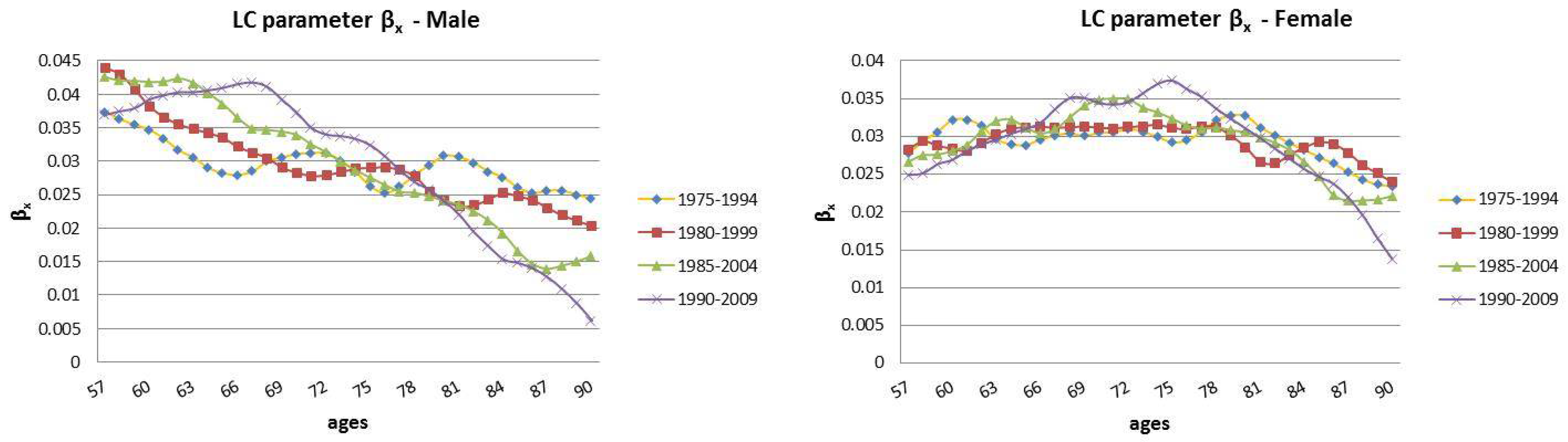
represents the average trend of mortality on the time horizon at age x;
  • β x represents a measure of the sensitivity in movement from the parameter k t . In particular, β x describes the relative speed of mortality changes, at each age, when k t changes; and
  • ε x , t is the homoskedastic error term, which incorporates historical trends not considered by the model. It is assumed to be ε x , t N ( 0 , σ ε 2 ) .
Appendix A illustrates the method adopted for the estimation and projection of the parameters.

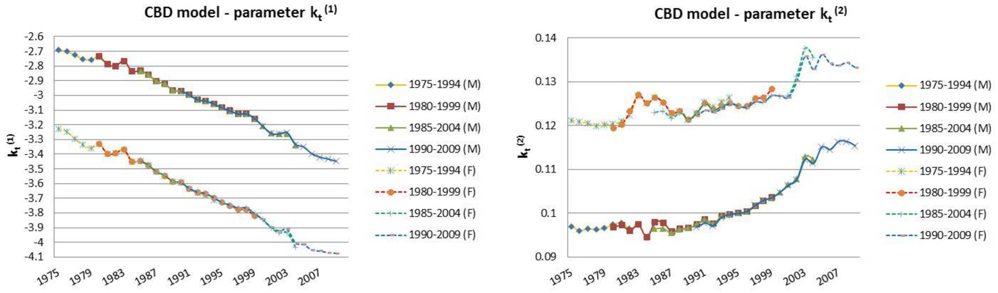
2.2. The Cairns–Blake–Dowd Model

We considered the original formulation of the model provided by Cairns et al. (2006) with the following model equation:
ln q x , t p x , t = k t ( 1 ) + k t ( 2 ) ( x x ¯ ) + ε x , t ,
where
  • k t ( 1 ) and k t ( 2 ) are two stochastic processes and represent the two time indexes of the model;
  • q x , t and p x , t represent, respectively, the death and the survival probability, at time t for an individual aged x;
  • ln q x , t p x , t = ln ( ϕ x ) = l o g i t q x , t is the logit transformation of q x , t , with ϕ x representing the mortality odds;
  • x ¯ is the mean age of the considered interval of ages; and
  • ε x , t is the error term that encloses the historical trend that the model does not express. All of the error terms are i.i.d following the Normal distribution with mean 0 and variance σ ε 2 .
The model is fully identified, so it does not require additional constraints.
Moreover, the time index k t ( 1 ) is the intercept of the model. It affects every age in the same way, and it represents the level of mortality at time t. More precisely, if it declines over time, it means that the mortality rate has been decreasing over time at all ages. The time index k t ( 2 ) represents the slope of the model: every age is differently affected by this parameter. For instance, if during the fitting period, the mortality improvements have been greater at lower ages than at higher ages, the slope period term k t ( 2 ) would be increasing over time. In such a case, the plot of the logit of death probabilities against age would become steeper as it shifts downwards over time (Pitacco et al. 2009).
Appendix B illustrates the estimation and projection methods involved.

3. Case Study: Italian Mortality Data from 1975 to 2014

The application of the presented models requires the use of the death probabilities time series for extrapolating mortality forecast. As already mentioned, we use data provided by ISTAT because these data are commonly used by private insurance companies and public pension providers. The range of ages is 57 x 90 . In particular, we chose the upper limit for taking into consideration the ISTAT graduation method of ending the life table (Istat 2001). The calculation of the probabilities of dying for ages over 95 is performed by extrapolating the q x , t graduated values following the Thatcher et al. (1998) model7:
q x , t = ϑ e γ x 1 + ϑ e γ x ; x 95 .
This kind of graduation could affect the backtesting results, comparing realized data with forecasts obtained by applying the LC (1) and the CBD (2) models, since they offer a different mortality pattern at old ages. For the ages from 5 to 94, ISTAT uses a moving average of crude rates with the length of seven values. Moreover, we selected the time period from 1975 to 2014 because, from in the mid-seventies in Italy, the successful fight against cardiovascular diseases began. More recently, efforts against tumors, which are still the main cause of death, have been launched. These successes have contributed to an extraordinary acceleration of growth in life expectancy, especially at higher ages: e.g., from 1975 to 2014, life expectancy at 60 years has seen an average increase of about four hours each day, both for men and women. In the male case, this phenomena extraordinarily occurred. Previously, life expectancy at birth had registered the first significant increase due to the control of infant and child mortality, while during the years under review, it has also benefited from the control of adult age mortality.
Currently, the probability of reaching an old age for a young adult is really high: for a 30 year old, the probability of reaching the age of 60 is almost 94% for males and 96.4% for females. However, it remains difficult to reach the threshold of 90 years, especially for men. Table 1 accurately shows8 how this probability changed starting from age 50. Moreover, it shows how the difference in probability between genders became greater as the age increased.
This process is known as the rectangularization and shift forward of the survival curves. Its measure can be derived from the entropy of a life table (Equation (4)). It was introduced by Keyfitz and Caswell (2005) and it is referred to in this paper as t H K , ξ with ξ the age by which the survival curve is built, and t the year of the period life table at which the entropy is computed (in our case t = 1975, 1976, ... 2014). Then,
t H K , ξ = j ( ln l j ) l j j l j ,
where l j is the probability of surviving from age9 ξ ( ξ = 0 , 1 , . ... , w ; l ξ = 1 ∀ ξ ) to age j ( j = ξ + 1 , ξ + 2 , w ). The entropy index becomes smaller whenever the survivorship curve l j moves towards a rectangular form; in this limit case, t H K , ξ = 0 .
Figure 1 shows how the trend of the rectangularization process has changed according to ages (i.e., from ξ = 50 to ξ = 65 , 75 ). Regarding women, this process was already in place before 1975. In particular, starting from ages 50 and 65, it is continued with a substantially linear continuity. In the case of men, the rectangularization process begins to escalate smoothly after 1984. However, the following trend shows a deep reduction of mortality, from which is derived an attenuation of the inequality between sexes even though it has not disappeared. In Figure 1, t H k , ξ shows that the mortality improvement in the elderly population has taken place at different rates over time, particularly with a faster steep decline for both sexes after 1993.
The differentiation of the pace in reducing mortality of both sexes starting from adult age up to those who are old is confirmed by the results of the Kullback and Leibler (1951) divergence:
t D K L , ξ ( h z , g z ) = z = 0 w ξ h z ln h z g z ,
where h z and g z are the probability distributions of the “time until death” random variable Z ξ for a person aged ξ , respectively, for males and females. Equation (5) measures the “difference” between these two probability distributions, which, in our case, is taken as the reference model g z . The choice is motived not only by the fact that mortality is significantly lower for women than for men, but also because the continuous decline of female mortality in the reporting period occurred much more regularly (Maccheroni 2014). The divergence in mortality between genders mortality has different characteristics depending on the considered age group.
Figure 2 shows that the divergence in mortality between sexes presents different characteristics, depending on the observed age. In particular, until 1981, the divergence gradually increased on the full range of ages. At a later time, differentials in mortality between sexes decrease whenever x is lower than 60, while they progressively increase at higher ages. These diverging trends make the application of the models interesting, especially for the comparison of results. Needless to say, the mortality forecast will be more accurate for women than men because women experienced a death risk reduction process with greater regularity than men.

4. Backtesting Analysis

In this section, we introduce the three different backtesting frameworks, and we present the related forecast results.
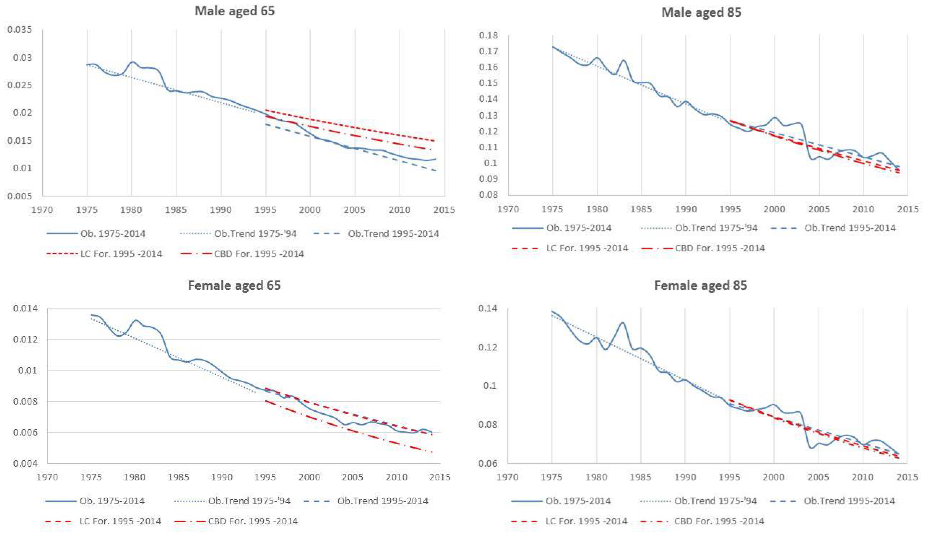
  • The fixed horizon backtest uses a fixed twenty-year historical “lookback” interval, 1975 t 1994 , and a fixed “lookforward” horizon, 1995 t 2014 (20 years).
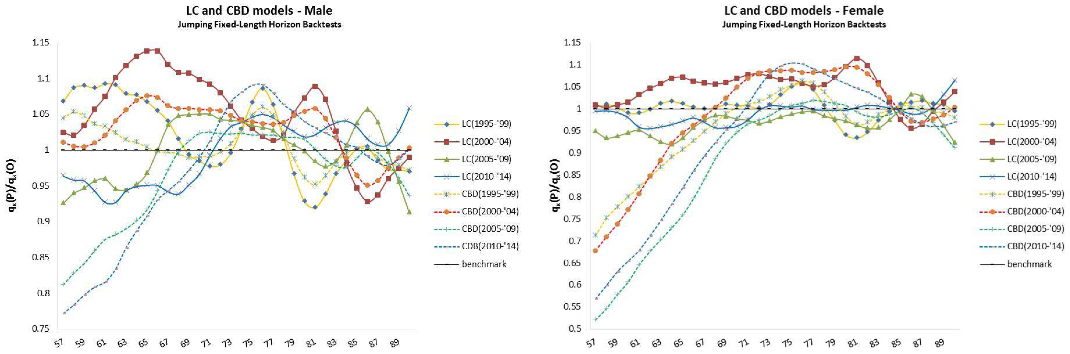
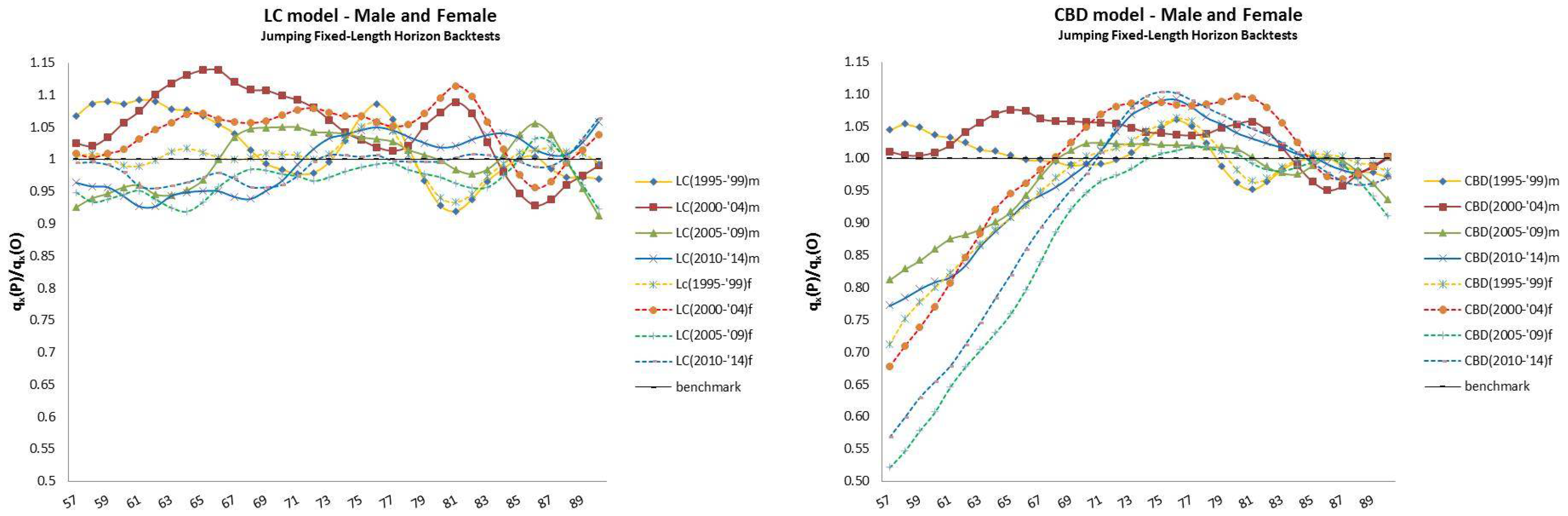
  • The jumping fixed-length horizon backtests make short run projections of five years10 and keep fixed the length of the “lookback” horizon (20 years), but make jumps of five years ahead to cover the “lookforward” interval, 1995 t 2014 . This analysis is divided into four groups of estimations and forecast, described in Table 2.
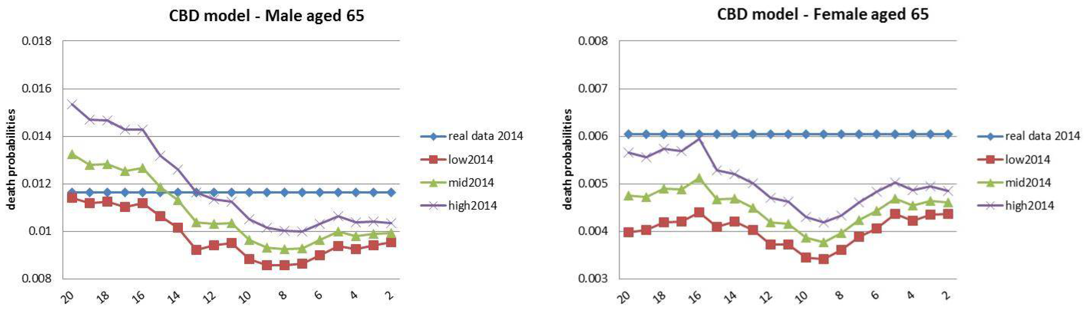
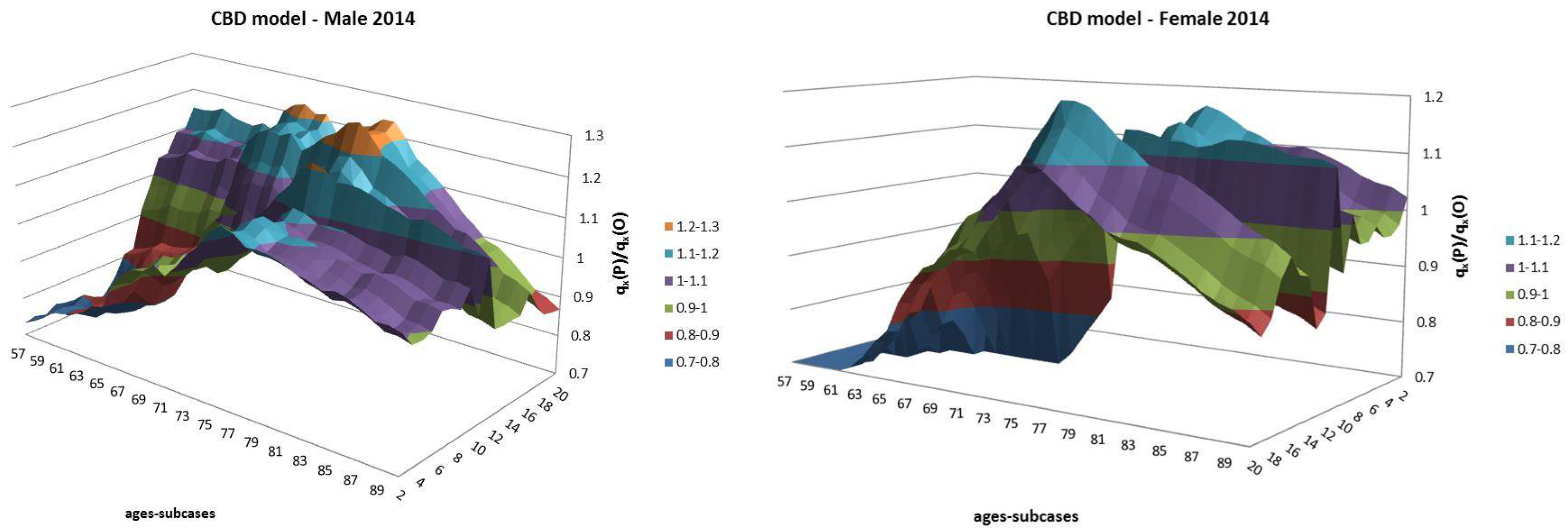
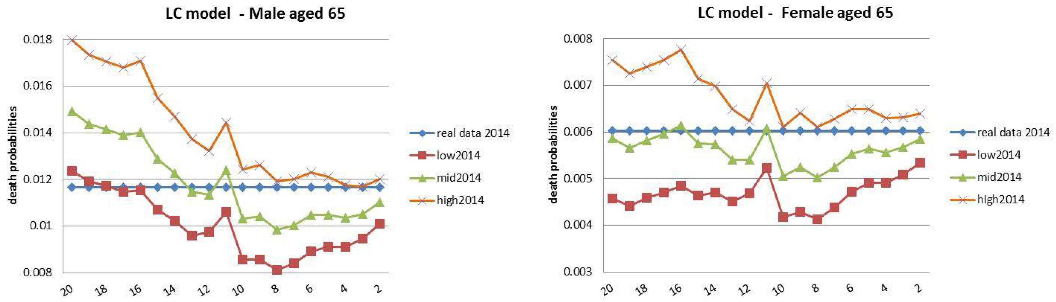
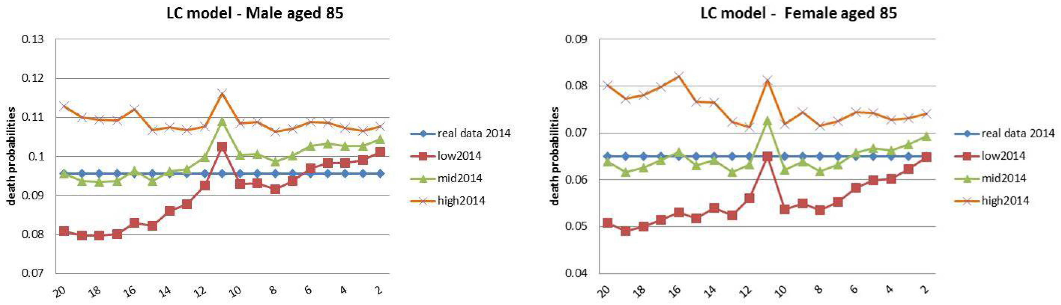
  • Finally, the rolling fixed-length horizon backtests keep fixed the length of the “lookback” horizon (i.e., 20 years) and let it roll ahead year by year. The projections are made over the remaining horizon, keeping fixed the last year of the projection at t = 2014 . This analysis is divided into nineteen groups of estimations and forecast, described in Table 3.
The numbers in parentheses show the length of the “lookforward” horizon. Moreover, they indicate the position of the year 2014 over the related projection interval. This will be particularly useful for the analysis of results that will be presented in Section 4.3.
Before going in depth about the backtesting analysis, we check for the estimation quality of the models over the historical “lookback” interval, 1975 t 1994 . For this purpose, we use the index Λ x 2 , a form of R 2 that particularly fits our case (Draper and Smith 2014), described as follows:
Λ x 2 = 1 1 n t ( q x , t O q x , t f t ) 2 1 n t ( q x , t O q x , t f t ) 2 1 n t ( q x , t O ) 2 1 n t ( q x , t O ) 2 ,
where q x , t f t is the fitted value for the q x , t and n is the total number of considered years (i.e., n = 20 ). The index provides the proportion of the temporal variance explained by the model for all 57 x 90 . Figure 3 shows that both models fit the observed data generally well. Particularly in the case of males, the share of the “explained variance” at any age is always greater than 88 % , while, for females, in the case of LC, it falls to 85 % at x = 63 . However, such a decrease takes place within a very limited age range between 61 and 65 years.
More specifically, by the analysis of the “explained variance” for both models, we see that the irregular path of the curves may be influenced by a cohort effect before the age x = 80 . This effect is diagonally observable on the graphs in Figure 4 for those individuals aged 57–59 in 1975 and 76–78 in 1994, respectively. These are the generations born during the First World War (1915-1918) who, in the course of their lives, have experienced higher mortality at the same ages than the previous and next cohorts (Maccheroni 2016). For ages older than x = 75 , the differences between the models are sharply evident. In particular, LC overestimates q x , t O and CBD underestimates (Figure 4).
Analysis of the projection results that will be presented in the next section shows that the described cohort effect has an impact on the forecast quality of the models in two ways.
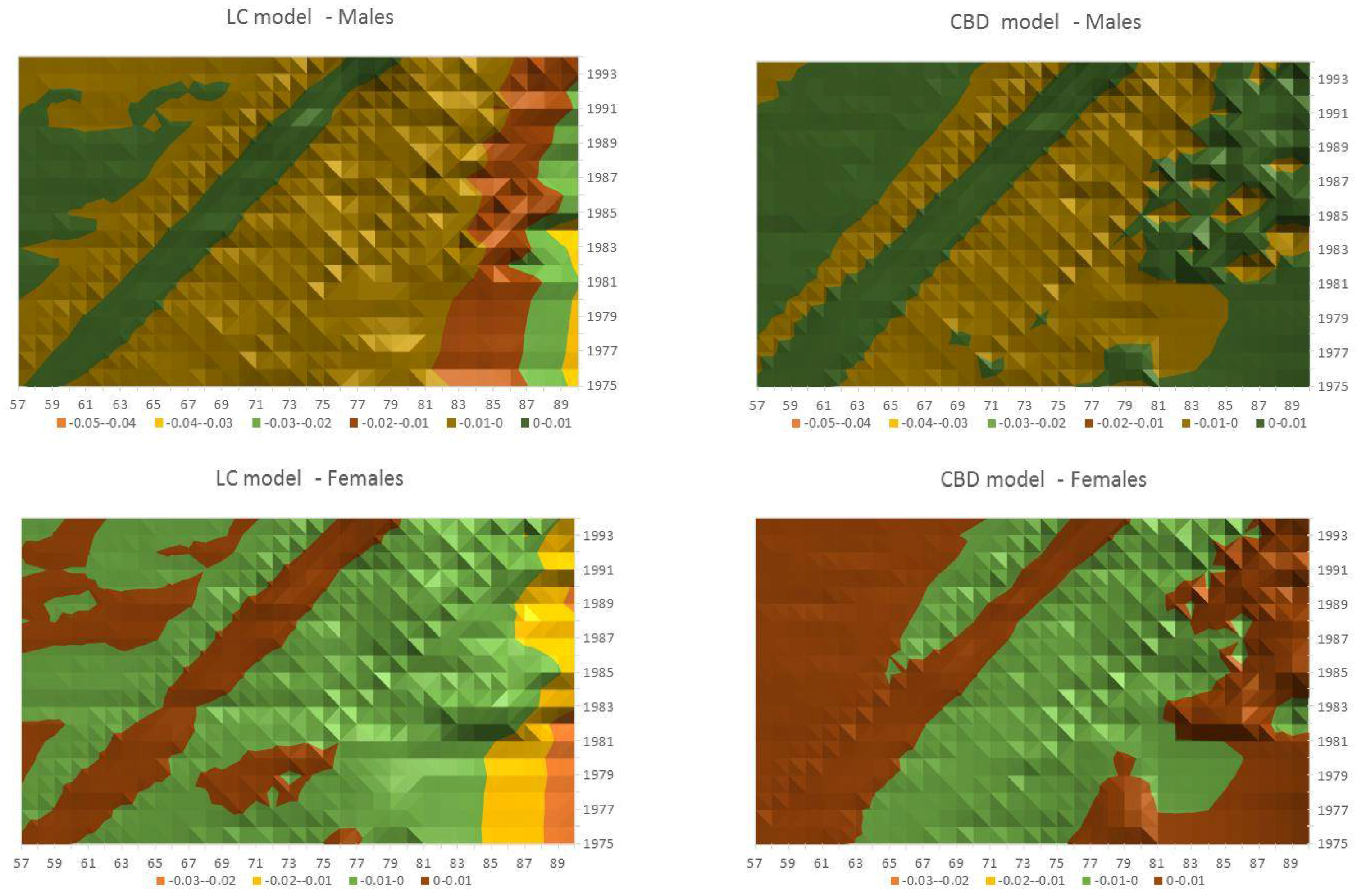
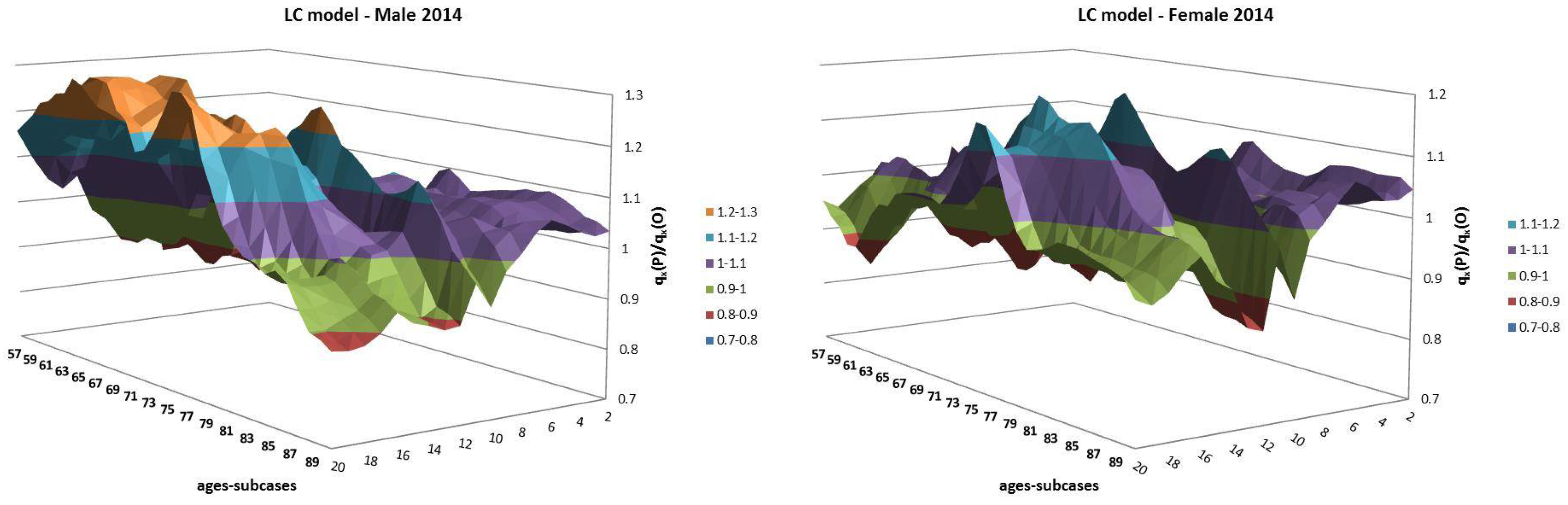
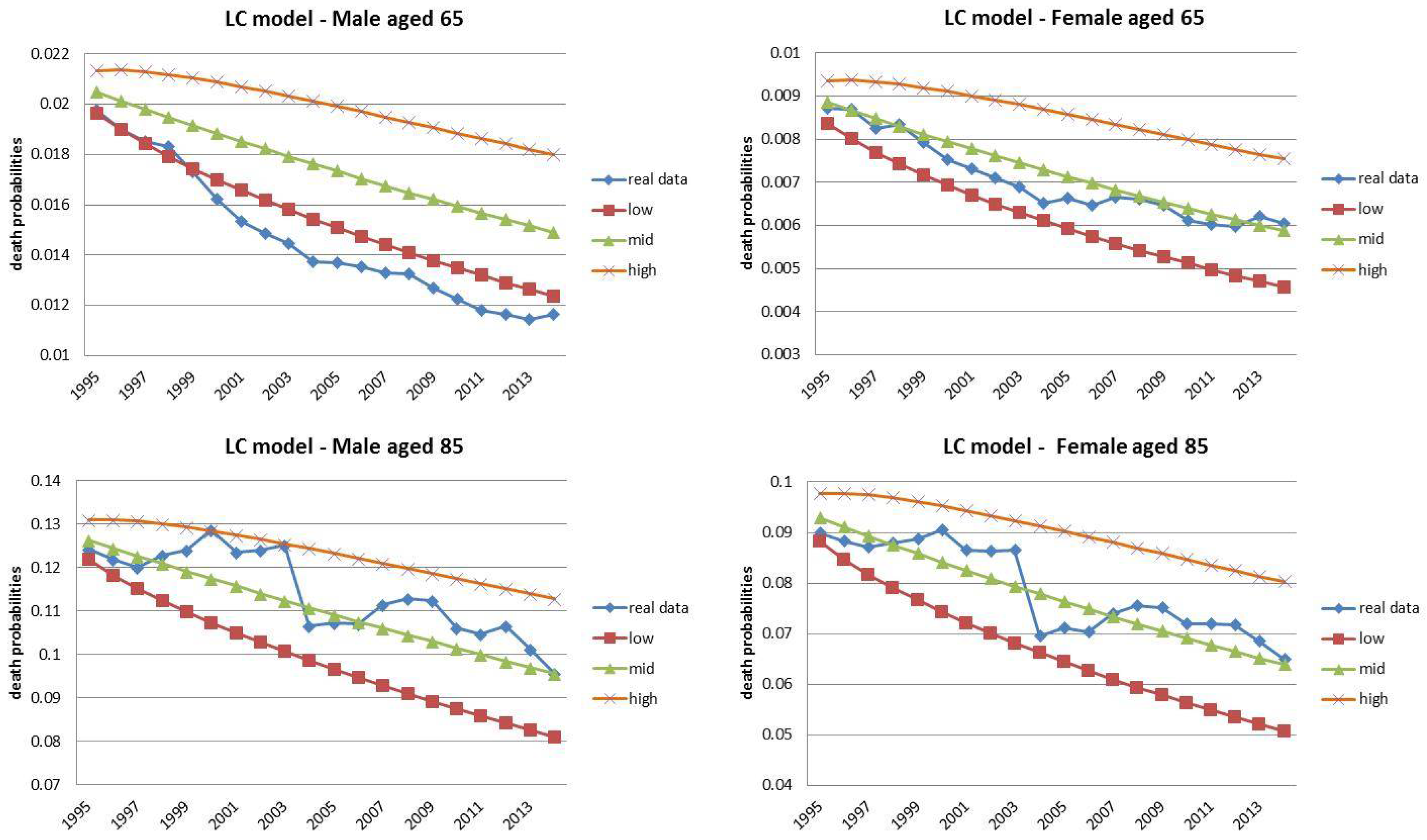
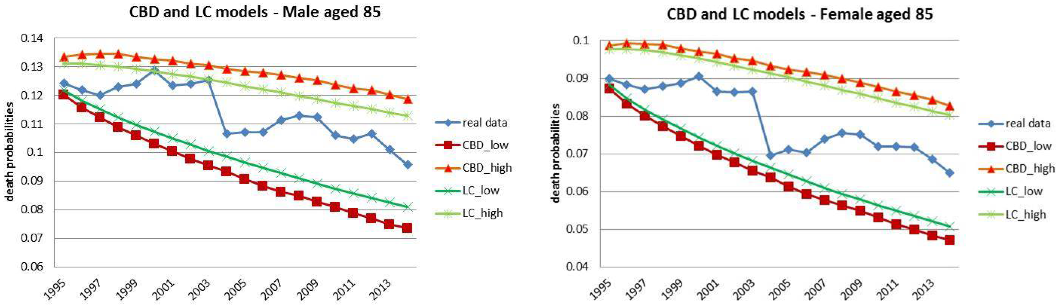
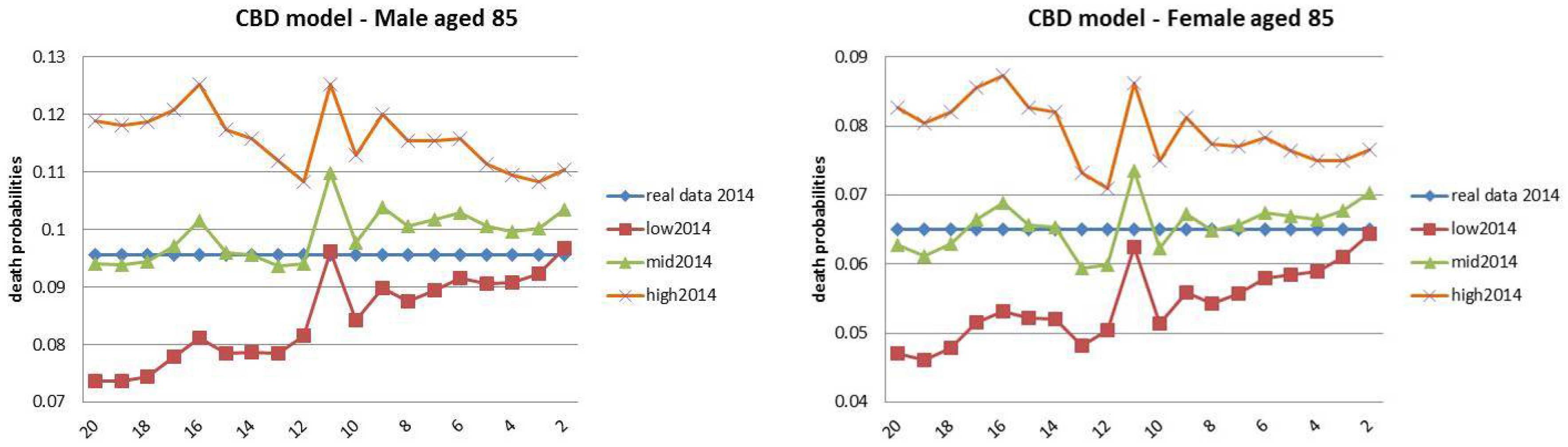
  • Both models slightly suffer the cohort effect for both populations over the projection horizon (1995–2014) for the same cohort aged 77–79 in 1995 that is no longer observed from 2006. In particular, both models show an underestimated forecast for such birth cohorts on both sexes with observed values above the upper limit of the confidence interval for some ages of the cohort. This occurred particularly for males.
  • The observed male q x , t for individuals aged 57–59 in 1995 and 76–78 in 2014, respectively, are often under the lower extreme of the forecast confidence interval. It seems that models have replicated the cohort effect over an homologous cohort in 1995, but since the male mortality evolution has changed consistently from 1975–1994 to 1995–2014, the two homologous cohorts (i.e., 57–59 in 1975 and 57–59 in 1995) showed different trends that lead to forecast errors. This scenario does not occur for females, since women experienced a more ordinary mortality evolution. Therefore, the homologous cohorts are similar, so the bias is not observable.
For these reasons, the results obtained with the three backtesting approaches need to be evaluated, taking into consideration the analysed cohort effect and its related impact on the forecast. In particular, forecasts seem to suffer the cohort effect as long as the data used for the estimation of the parameters take into account years from 1975 to 1985. After 1985, the cohort effect is small compared to the overall sample; therefore, projections do not suffer greatly from it.

4.1. Fixed Horizon Backtest (1995–2014)

The first backtesting analysis takes into account a forecast horizon that is demographically considered a medium-term projection horizon. The comparisons proposed are among the most likely values of q x , t P prediction, which is the projected central value derived by the model on which we constructed the 95% confidence interval and those observed q x , t O ; comparisons between the central value and extremes of the confidence interval occur only for the ages 65 and 85. These are the ages that in the demographic literature mark the entrance in the range of so-called “young-old” and “oldest-old”. Unfortunately, due to space limitations, it was not possible to present the comparison to the age of 75, which divides the old from the “young-old” (Vaupel 2010).
The q x , t O can present a strong temporal variability due to the observed cohort effect and to the so-called “period effect”, which is the time condition that affects mortality via a variety of factors. Among these, the best known is the climatic effect that can, for instance, cause a rise in mortality at old ages during a very hot summer (e.g., an episode occurred in Italy in 2003), or epidemiological effects that arise from flu in winter in low-mortality countries. Needless to say, the impact of those factors is stronger on the most vulnerable people. For this reason, a rise in mortality due to those factors is generally followed by a decrease in mortality, since those who remained alive have a lower frailty level. These mortality shocks can affect short-term forecasts rather than medium-term ones, since the latter are usually more capable of capturing changes in environmental and socio-economic conditions and people’s lifestyles.
From an applicative point of view, particularly focused on the insurance and social security sector, we were interested in analysing the performance of the models on assessing the risk of death at various ages. It is from this point of view that we are going to develop our analysis. For this purpose, we make a brief assessment of forecast errors that was performed using as an index the Root Mean Squared Errors (RMSE), defined as follows:
R M S E = M S E ,
with
M S E = 1 υ x t ( q x , t O q x , t P ) 2 ,
where the mean squared errors (MSE) are equal to the sum of squared errors adjusted for the residual degrees of freedom υ . Moreover, q x , t O and q x , t P are, respectively, the death probabilities observed and forecast (projected). We use the root of the adjusted SSE to take into account the difference in the number of free parameters between the models. Table 4 shows R M S E for the first and the second backtesting approach that will be presented in the following section. Moreover, it takes into account exclusively the central value of the confidence interval as the most relevant for pension policy-makers and annuity providers (Whitehouse 2007).
Table 4 shows how the LC model proposes a more accurate forecast with respect to the CBD model for the period 1995–2014 for females; it is more difficult to judge the models’ performances for males given the small difference between the RMSE results. These predictions are produced on the extrapolated parameters k t (Appendix Equations (A7) and (A9)), but the result is made more flexible by the stochastic component of the models that allows building of the forecast confidence interval. One cause of error can arise from the fact that the central value of the projection may be shifted with respect to the observed data, even though it does not differ from the observed trend recorded over the projection horizon. Figure 5 provides a graphic explanation of the phenomenon. In particular, for individuals aged 65, the male forecasts 1995–2014 are above the mortality trend observed for the same period, with divergent paths for the LC model. In the female case (age 65), only the CBD model shows divergences. However, these deviations may be instead very low, as in the case of the LC model for females aged 65, or in the case of both models for both sexes aged 85 (Figure 5). Moreover, the bias due to the continuing fluctuations of the risk of death over time has to be taken in consideration. The confidence interval provided by the two models takes into account this stochastic component of mortality (Figures 7 and 9), although this may occur with different levels of precision (Figure 10).
Figures 6 and 8 show the overall error dynamic highlighted by the ratio between the projected q x , t P and the observed q x , t O .
As far as men are concerned, the LC model initially overestimates q x , t O from ages 57 to 80 (approximately), with persistence across years. In particular, the overestimation errors become sharply evident as the projection is extended to the last year of the forecast horizon. Figure 6 multi-dimensionally shows the ratio between projected and the real death probabilities. The described LC performance trend is also graphically reported by the Figure 7, comparing projections at ages 65 and 85 to the observed data. The overestimation starts decreasing from age 80, pointing out that the divergence between q x , t O and q x , t P is really close to zero. However, for high ages at the extreme of the interval, LC forecasts systematically underestimate q x , t O .
As for women, the divergence between q x , t O and q x , t P is sharply smaller than for men. This is particularly evident in Figure 6, which shows that the forecast initially underestimates real data converging at the age 65 and then starts overestimating for a wide span of ages. Furthermore, the last part of the age range is again characterized by an underestimation path. However, the overestimation experienced at higher ages is smaller than the one observed in the male case.
The CBD forecast greatly overestimates the male mortality historical evolution, particularly for the central and last years of projection. The error is evident in the full range of ages, although it becomes smaller at the age 80, after which forecasts start underestimating q x , t O with an increasing magnitude until the last age and the last projection year (i.e., x = 90 and t = 2014 ) (Figure 8).
When we look at the female case, the accuracy of the CBD forecast is worse. In this case, in fact, we can notice a wide and systematic underestimation on approximately all of the first half of the age range for almost the totality of the forecast horizon. In particular, the forecast error reduces around the age 68, then it starts overestimating until x = 85 , after which it underestimates again. However, at x = 85 , the forecast is relatively accurate, with values of q x , t O all inside the confidence interval (Figure 9).
In conclusion, both models make similar forecast errors. On the one hand, regarding males, the error is represented by an initial overestimation that smoothly converges to the real data and then starts underestimating, although the divergences experienced with the CBD model are characterized by a smaller variability with respect to the LC model. On the other hand, the female case shows an initial underestimation converging to the real data and then a fluctuation of overestimation and final underestimation. In general, the LC model provides a better fit over a wide range of ages, showing lower variability in both over and underestimation.
In any case, the choice between the models becomes difficult at particular ages. Figure 10 shows the high and low confidence intervals for both models. Even though LC curves are nested into the CBD lines with greater differences shown in the male case, both models’ confidence intervals include the observed data, providing theoretical robustness to the projections.

4.2. Jumping Fixed-Length Horizon Backtests

From the results shown in Table 4, it is clear that the two models best capture the trend of female mortality. More specifically, the accuracy of the prediction about the next five years, using the periods 1975–1994 and 1990–2009 as the database, is far higher than the other two sub-groups of forecast. On the contrary, neither model shows the underestimating and overestimating path of the q x , t O at various ages, which was peculiar in characterizing the result in the previous backtesting case. Only the results of the CBD model show a similar pattern, although in this case with overestimates and underestimates staggered by age differently from period to period. This point will be discussed in detail hereafter.
The analysed models should be assessed on a long-term prediction, but in this case, it is particularly noticeable how a change in the starting point of the time series makes the models differently incorporate the changes in mortality that occurred in the past 20 years. This is generally accomplished through the parameter estimates, which are also reflected throughout the extrapolation process associated with the model. However, an estimation procedure cannot guarantee a priori a constant performance of the forecast. This is also due to the fact that the dynamic of mortality varies in accordance with a multiplicity of social factors that affect the life of every person. Unfortunately, mathematical models are not always able to capture such factors11. “We conclude that the deviations from exponential law at young ages can be explained by heterogeneity, namely by the presence of a subpopulation with a high initial mortality rate presumably due to congenital defects, while those for old ages can be viewed as fluctuations and explained by stochastic effects” (Avraam et al. 2013, p. 1).
Now, we analyse the immediate effects of these estimates, starting with the LC model (1). The parameters α x and β x are time-independent age-specific constants, so their estimations will depend on the historical period used as the database and do not need to be predicted. The k t index captures the time-series common risk factor in that same period, showing the main mortality trend for all ages at time t. Forecasts are produced by extrapolating the time index k t , and the mortality projections at each age are all linked together by the product12 β x k t (1).
In this backtesting framework, the shift forward of the database shows a continuous decline in mortality provided by the estimates of the parameter α x and k t . Moreover, the estimations for the parameter β x referring to the male case show greater values at the beginning of the age range ( 57 x 90 ) than at the end. This result describes a greater decrease in mortality for those ages with respect to the others, at which β x presents smaller estimated values (Figure 11, male).
This scenario is in line ex ante with the historical experience. However, the forecast for the period 2000–2004 shows a systematic overestimation of the q x , t O for both men and women until the age x = 80 (Figure 12, LC model). Taking into consideration the female case, the estimates of the parameter β x are more susceptible to changes in the starting point of the time series. Figure 11 shows this for the female case. Needless to say, the female β x trend improved the accuracy of the forecast for the periods 1995–1999 and 2010–2014 (Figure 12, LC model).
In the case of CBD model (2), the presence of two time-varying parameters k t ( 1 ) and k t ( 2 ) should increase at least a priori the forecasting performance with respect to the LC model. This result is evident for the male forecast in the short-run (Table 4). As mentioned, in the CBD model, the k t ( 1 ) mortality index represents the level of the mortality curve, after the logit transformation. A reduction in k t ( 1 ) entails a parallel downward shift of the logit-transformed mortality curve, which represents an overall mortality improvement. In particular, this is what occurred in practice, with greater effects for the female case that are enhanced by the smooth divergences of k t ( 1 ) trends between sexes. This is clear on the left-hand side of Figure 13 below, in which we also checked for the new-data-invariant property of the model (Chan et al. 2014).
In this case, the jumps of five years ahead do not seem to affect the k t ( 1 ) trend. This is also evidenced by the substantial continuity of the overall reduction in mortality. This is not the case as far as the the k t ( 2 ) mortality index is concerned. Its path drafts the slope of the logit-transformed mortality curve. An increase in k t ( 2 ) entails an increase in the steepness of the logit-transformed mortality curve, which means that mortality at younger ages i.e., those below the mean age x ¯ (here x ¯ = 73.5 ) improves more rapidly than at older ages. This is clear on the right-hand side of Figure 13. Regarding the male case, we find that the speed of increase in k t ( 2 ) is greater for the periods 1985–2004 and 1990–2009 than for the other two. For this reason, the projected q x , t P shows stronger improvements in mortality for the periods 2005–2009 and 2010–2014 than for the others, particularly for the ages lower than x = 69 . More in depth, results show an underestimation of the q x , t O for the ages lower than x = 69 and a smooth overestimation path for those higher. Despite the fact that the growth of k t ( 2 ) between 1980 and 1999 is higher than that of 1975–1994 and that the reduction of k t ( 1 ) is greater, we find that q x , t P sharply overestimates q x , t O in the period 1995–1999 and particularly in 2000–2004 for the full range of ages.
Regarding women, k t ( 2 ) presents similar records to men, whereas for the period 1990–2009, the growth rate of k t ( 1 ) is slightly attenuated. In contrast with the male scenario, in this case, q x , t P systematically and significantly underestimates q x , t O from the age x = 57 , converging gradually to the observed data as x moves towards x ¯ . Moreover, Figure 14 shows that the underestimations are larger for the projection periods 2005–2009 and 2010–2014. This error path does not influence the forecasts of ages higher than x ¯ that generally overestimate q x , t O . In particular, for ages higher than x ¯ , forecasts of the periods 1995–1999 and 2010–2014 show better results than those of the other two projection windows (Figure 12, CBD model).
Hence, comparatively, we conclude that a good result for the performance index RMSE (Table 4) can hide some compensation for the forecast error in terms of age and time. Figure 14 graphically shows the described scenario.

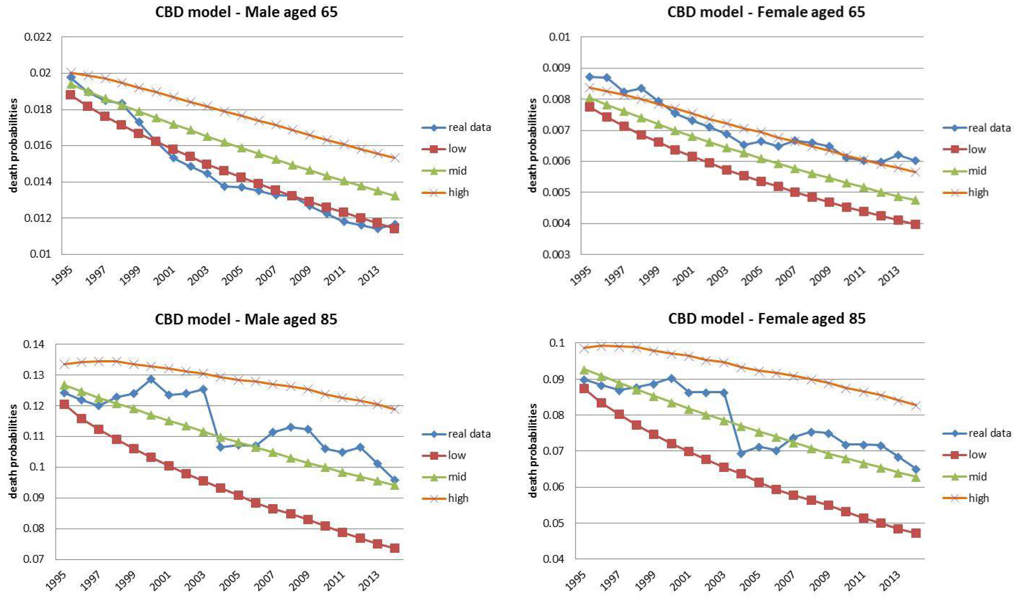
4.3. Rolling Fixed-Length Horizon Backtests

Finally, the analysis concludes with the study of the forecast convergence to the observed q x , t O in the year13 2014. For this reason, we build a framework of 19 groups of estimations and projections, rolling the database (fixed-length of 20 years) sequentially forward from14 1975 to 1993. Then, we compare the 2014 forecast obtained in each group with the realized mortality for that year. We observe that the comparison enhances the same critical issues analysed in the previous paragraphs, with particular emphasis on two main aspects.
Firstly, scrolling the database over time year by year gives rise to strong fluctuations in the performance of the prediction measured by the ratio of q x , t P and q x , t O . These oscillations (Figure 15 and Figure 16) are evident for both sexes in the results of both the LC and the CBD models. Moreover, the trend is interrupted by a deep break in correspondence of the 1985–2004 database. In particular, the previous base (1984–2003) provided a strong overestimation of q x , t O especially at old ages. The base 1985–2004 data has then reduced the size, while the next one (1986–2005) moved closer to q x , t O .
One the one hand, this result may be related to the cohort effect described at the beginning of paragraph 4, since the cohort effect is proportionally greater on the base of data including years before 1985. On the other hand, they can be partially justified by also recalling that the year 2003 was characterized by a sharp rise in mortality, especially at old ages. Therefore, this historical event may have affected the estimated parameters. However, in the male case, both models systematically underestimate q x , t O when the age is lower than x = 73 , and overestimate when it is higher.
This result is particularly evident when the “lookback” horizon is 1985–2004, and also for the following cases. In particular, CBD underestimates when the database refers to the period 1981–2000. However, for the period 1985–2004, the divergence becomes greater compared to the LC model (Figure 15 and Figure 16). As is shown, the choice of the database plays a crucial role in forecasting mortality.
Figure 15 shows the ratio between the projected and observed death probabilities for the year 2014. Table 3 shows the projections obtained for that year on each pair of “Lookback” and “Lookforward” horizons.
In particular, the sub-case index of the graph shows the position of that year on the projection horizon (i.e., 20 means that the year 2014 was the 20th year of the projection, 19 means the 19th, and so on ). Since the dataset is rolling over time and decreasing the projection horizon, we decided to show the position of the year 2014 to take into account both the specific sub-case and the related length of the forecast horizon. Figure 16 shows the same for the CBD model with an inverted order of sub-cases for males to better show the shape of each curve.
Secondly, we detected substantial differences between the performances of the two models by analysing female mortality. Figure 16 shows how the CBD model systematically underestimates real mortality until the age of 75 and then starts converging to q x , t O after that “threshold” age. This result, which was already evident in the previous analysis, is likely linked to the combined effects on the CBD model (2) of the role of the mean age x ¯ (in our case x ¯ = 73.5 ) of the age group, for which the forecast is made, and of the observed female mortality pattern. These results are also confirmed from the analysis of the confidence interval referred to the forecast. Figure 17 shows that, in the female case at age 65 ( t = 2014 ), q x , t O is always outside the confidence interval, while at age 85, it is inside with central values almost converged to the real data in each sub-case (Figure 18). In the case of the LC model, the initial underestimation of the q x , t O is much less pronounced with respect to the previous case. Moreover, the “threshold” age, with respect to which the forecast underestimates and then overestimates q x , t O , increases as the database moves forward (Figure 15).
Figure 17 and Figure 18 show the convergence of the projections to the observed data for the year 2014, at ages 65 and 85. The x-axis shows the position of the year on the forecast horizon as before. Figure 19 and Figure 20 present the same for the Lee–Carter model.

5. Conclusions

The main aims of this paper are to scrutinize the forecast for both sexes proposed by the original formulation of the models, given the wide use of LC at the national level, and to analyse the long-term forecast with respect to the short term, observing qualitative differences in the estimation of the parameter accordingly to changes in the starting point of the database.
Regarding the former, we find that, basically, neither model was able to capture the shock in terms of improvements on the male mortality trend, with greater biases for ages lower than x = 75 , which were those more affected by the improvement. In this sense, CBD forecasts for those ages are more biased than LC projections in terms of overestimations. The limited capacity of the models to predict male mortality is evident in all of the three backtesting frameworks. Table 4 numerically summarizes the difference in terms of performances between sexes for the first two backtesting approaches. In addition, the analysis of the forecast for the year 2014 that we provided with the third approach confirms this result. Moreover, women’s forecasts are widely more accurate than men’s, with small biases observed both in the short and the medium-term. However, in the female case, CBD projections showed particularly deep and systematic underestimations with respect to ages lower than 75.
From the comparison between the short-term and the medium-term forecast, we find that changes in the starting point of the database widely affect the estimation of the LC parameters, particularly for β x with observable impacts on the projections. The female forecasts are more influenced by those changes in β x . The CBD model satisfies the “new-data-invariant” property for the estimation of the parameter k t ( 1 ) , while k t ( 2 ) presents persistent changes for the same year as the dataset slides forward. This aspect is more evident in males than in females. In particular, the adjustment of the parameter k t ( 2 ) (i.e., x x ¯ ) affects mortality forecasts with weights of the opposite sign at the extremes of the considered age range. The weight is greater the larger the age range. This structural characteristic of the model, albeit simultaneously with k t ( 1 ) , results in a systematic underestimation of the q x , t O for ages lower than x ¯ that gradually decrease as x moves towards x ¯ . Moreover, mortality forecasts around x ¯ are almost exclusively explained by k t ( 1 ) , since ( x x ¯ ) is really close to 0 in that case. On the contrary, as x gets closer to the upper limit of the age range, the weight of ( x x ¯ ) on mortality forecasts changes with the opposite sign, with resulting overestimation of the q x , t O . For these reasons, the risk in terms of application of the models is conspicuous because it could potentially affect both the mortality risk and the longevity risk. Taking into consideration the variability of both the parameters β x (LC) and k t ( 2 ) (CBD), it is difficult to judge a priori what these two rigidities penalize more in the mortality forecast.
As far as the CBD model is concerned, we find that projections are not reliable for describing mortality at ages before x = 75 . For this reason, LC projections are preferable for describing Italian mortality in this particular framework of years and ages. However, CBD forecasts showed a more restrained variability of the forecast error at higher ages with respect to LC. This result and the fact that usually the CBD confidence interval at higher ages is wider (i.e., LC is nested in CBD) than LC ones provide a more accurate theoretical robustness to the CBD for ages greater than x = 75 .
We would like to make clear that we examined the models in their original form, so we cannot rule out the possibility that some extensions of the models might resolve these issues on Italian data (1975–2014). In particular, we expect that the results of both models may be improved with the adoption of the model extensions, including a cohort component, in order to reduce the bias caused by the cohort effect of those born during the First World War. Moreover, the CBD extension, including the quadratic term of the age component, may solve the weighting issue of the model over the considered interval of ages on this data.
In conclusion, the results seem to be relevant for private and public Italian annuity providers that use LC forecasts as demographic bases. From this perspective, the choice between the two models may vary in accordance with the purpose of the use of the model (e.g., the age and the sex of the insured). Even though we limited our analysis to the study of the forecast q x , t , we can infer that a backtesting analysis of annuity prices, based on the forecast obtained by the original formulations of the models, would show evidence of a distortion caused by the forecast error on the money’s worth of an annuity and on reserves.

Acknowledgments

The authors want to thank the Center for Research on Pensions and Welfare Policies (CeRP) for supporting this study. It is one of the CeRP’s contributions to the hackUniTO research project about aging, promoted by the University of Turin.

Author Contributions

The authors contributed equally to this work.

Conflicts of Interest

The authors declare no conflict of interest.

Appendix A. Lee–Carter Estimation and Projection

Appendix A.1. Parameter Estimations

The parameter estimation was computed with respect to the Ordinary Least Square (OLS) estimation method in accordance with the original approach suggested by the authors.
The following constraints were used to find a unique solution for the parameters:
x = x 1 x m β x = 1 a n d t = t 1 t n k t = 0 .
To obtain the estimation for the variable α ^ x , it was necessary to compute the partial derivative of the equation L S ( α , β , k ) = x t ( ln ( m x , t ) α x β x k t ) 2 , with respect to α x . Then, as a first order condition, we get:
α ^ x = 1 t n t 1 + 1 t ln ( m x , t ) ,
where the denominator simply represents the number of years considered in the dataset, and x = x 1 , ... , x m is the considered range of ages. As is expressed by the Equation (A2), the estimation for the first parameter α x was given by the average of the logarithms of the central rate of mortality over time t. Furthermore, the estimations of β ^ x and k ^ t for the parameters β x and k t were obtained by adopting the Singular Value Decomposition of the matrix A of elements ( ln m x i , t j α x i ) , with i as age index and j as time index (years considered in the data).
At this point, the estimated parameters were recalibrated so the differences between the actual and the estimated total deaths in each year were zero. This implies that the recalibrated k ^ t * solves the equation15:
x d x , t = x e ( α ^ x * + β ^ x * k ^ t * ) L x , t .
Finally, the estimated parameters were adjusted to satisfy the constraint at (A1) for the parameter k ^ t * . Then:
a x * = α ^ x + β ^ x k ¯ ,
β x * = β ^ x j = 1 x m x 1 + 1 β ^ 1 j ,
k t * = ( k ^ t * k ¯ ) j = 1 x m x 1 + 1 β ^ 1 j ,
where k ¯ = 1 t n t 1 + 1 t = 1 t n k ^ t * is the arithmetic average of k ^ t * with respect to time t, and j = 1 x m x 1 + 1 β ^ 1 j is simply the sum of all the estimated β ^ , which sum to 1. The fitted model is then used to estimate the median and the 95 % prediction interval.

Appendix A.2. Parameter Projection

We projected the estimated16 parameters k t * of the Lee–Carter model using a Random Walk with Drift equation:
k t = k t 1 + d + η t w i t h η x , t N ( 0 , 1 ) a n d E ( η s , η t ) = 0 ,
where the drift d is estimated by the formula:
d ^ = ( k 2 * k 1 * ) + ( k 3 * k 2 * ) + ... + ( k T * k T 1 * ) t n t 1 = ( k T * k 1 * ) t n t 1 ,
with k T * and k 1 * , respectively, given by the first and the last elements of the vector k t * = [ k 1 * , ... , k T * ] . The drift is simply the arithmetic mean of the differenced series of estimated parameters.
After having solved Equation (A7) of the RWD model, we describe the projection of the parameter k t at time T + Δ t as follows:
k ^ T + Δ t = k T * + ( Δ t ) d ^ + Δ t η t .
At this point, it was possible to get the equation for the projection of the central rates of mortality as follows:
m ^ x , T + Δ t = e a x * + b x * k ^ T + Δ t .
Finally, we transformed the central mortality rates into probabilities by adopting the Reed and Merrell (1939) method. The relation is expressed by the equation:
n q x , t = 1 e n ( m x , t ) n 3 0 . 008 ( m x , t ) 2 .

Appendix B. Cairns–Blake–Dowd Estimation and Projection

According to the original formulation of the model proposed by Cairns et al. (2006), Equation (2) is the result of the logit transformation of the following model equation:
q x , t = e k t ( 1 ) + k t ( 2 ) ( x x ¯ ) 1 + e k t ( 1 ) + k t ( 2 ) ( x x ¯ ) .
Fitted values for the stochastic processes k t ( 1 ) and k t ( 2 ) were obtained using least squares applied to the Equation (A8). The fitted model is then used to estimate the median and the 95 % prediction interval.
The parameters vector k t = k t ( 1 ) , k t ( 2 ) has been projected by considering the following equation of a two-dimensional random walk with drift:
k t + 1 = k t + μ + C N ( t + 1 ) ,
where
  • μ is a constant 2 × 1 vector of drifts, computed as the arithmetic mean of the differenced series of estimated parameters;
  • C is a constant 2 × 2 upper triangular matrix, derived by the unique Cholesky decomposition of the variance–covariance matrix V = C C of the parameters vector k t + 1 ; and
  • N ( t + 1 ) is a two-dimensional standard normal random variable.
The adopted forecast method treats the estimated parameters as if they were the true parameter values (parameters certainty). In particular, the presented projections were computed17 considering parameter certainty based on 5000 simulation trials.

References

  1. ANIA. 2014. Le Basi Demografiche Per Rendite Vitalizie a 1900–2020 e a62. Technical report. Roma: Associazione Nazionale fra le Imprese Assicuratrici (ANIA). [Google Scholar]
  2. Avraam, Demetris, Joao Pedro de Magalhaes, and Bakhtier Vasiev. 2013. A mathematical model of mortality dynamics across the lifespan combining heterogeneity and stochastic effects. Experimental Gerontology 48: 801–11. [Google Scholar] [CrossRef] [PubMed]
  3. Booth, Heather, Rob Hyndman, Leonie Tickle, and Piet De Jong. 2006. Lee-carter mortality forecasting: A multi-country comparison of variants and extensions. Demographic Research 15: 289–310. [Google Scholar] [CrossRef]
  4. Cairns, Andrew J. G., David Blake, and Kevin Dowd. 2006. A two-factor model for stochastic mortality with parameter uncertainty: Theory and calibration. Journal of Risk and Insurance 73: 687–718. [Google Scholar] [CrossRef]
  5. Cairns, Andrew J. G., David Blake, Kevin Dowd, Guy D. Coughlan, David Epstein, Alen Ong, and Igor Balevich. 2009. A quantitative comparison of stochastic mortality models using data from england and wales and the united states. North American Actuarial Journal 13: 1–35. [Google Scholar] [CrossRef]
  6. Chan, Wai-Sum, Johnny Siu-Hang Li, and Jackie Li. 2014. The cbd mortality indexes: Modeling and applications. North American Actuarial Journal 18: 38–58. [Google Scholar] [CrossRef]
  7. Dowd, Kevin, Andrew J. G. Cairns, David Blake, Guy D Coughlan, David Epstein, and Marwa Khalaf-Allah. 2010a. Backtesting stochastic mortality models: An ex post evaluation of multiperiod-ahead density forecasts. North American Actuarial Journal 14: 281–98. [Google Scholar] [CrossRef]
  8. Draper, Norman R., and Harry Smith. 2014. Applied Regression Analysis. New York: John Wiley & Sons. [Google Scholar]
  9. Istat. 2001. Tavole di mortalità della popolazione italiana per provincia e regione di residenza. anno 1998. Roma: Servizio Popolazione Istruzione e Cultura. [Google Scholar]
  10. Istat. 2008. Previsioni demografiche. 1 gennaio 2007-1 gennaio 2051. Nota informativa, Popolazione. Technical report. Roma: Istat. [Google Scholar]
  11. Istat. 2016. Indicatori Demografici: Stime Per L’anno 2015. Technical report. Roma: Istat. [Google Scholar]
  12. Keyfitz, Nathan, and Hal Caswell. 2005. Applied Mathematical Demography. New York: Springer, vol. 47. [Google Scholar]
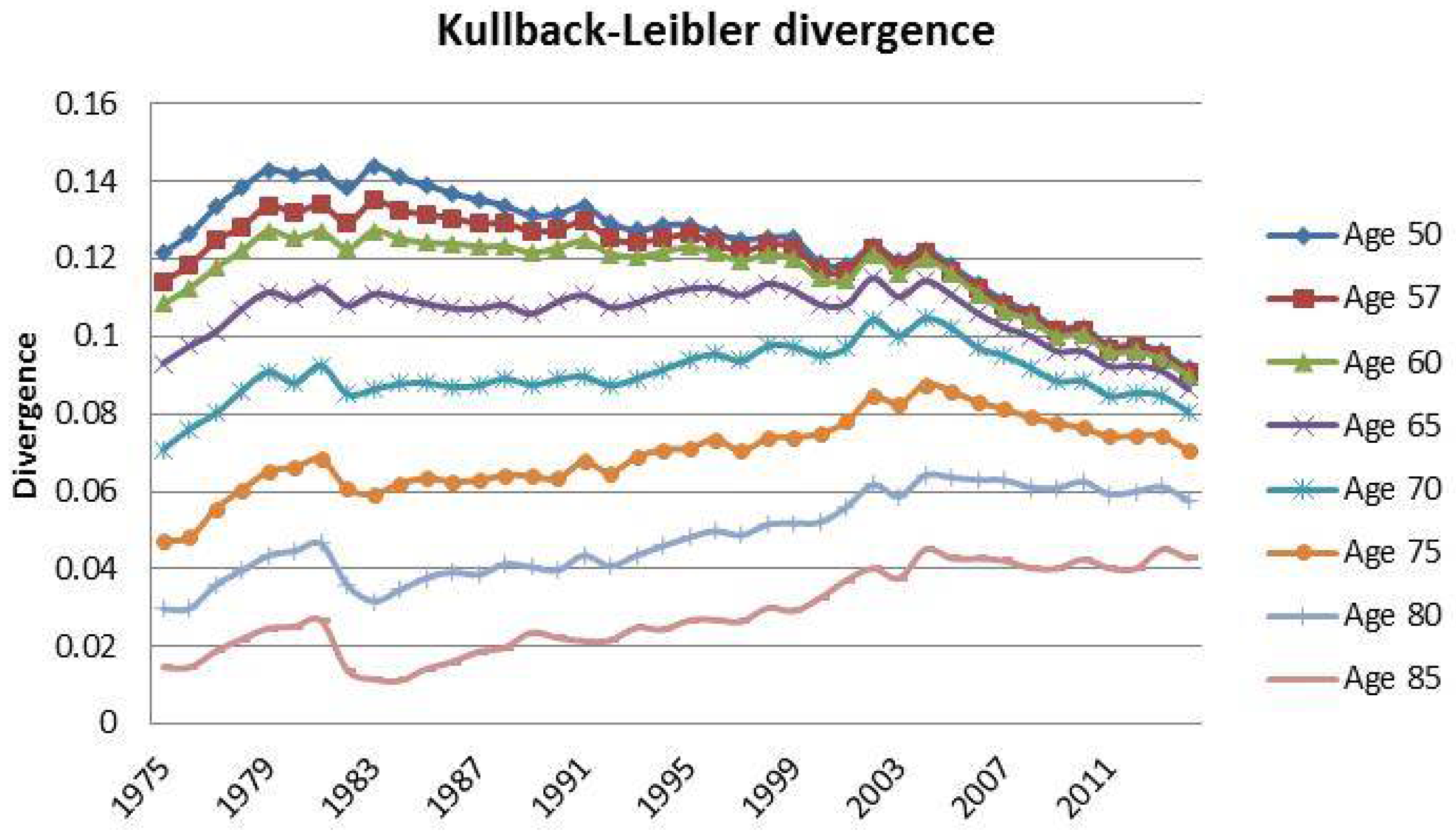
  13. Kullback, Solomon, and Richard A. Leibler. 1951. On information and sufficiency. The Annals of Mathematical Statistics 22: 79–86. [Google Scholar] [CrossRef]
  14. Lee, Ronald. 2000. The lee-carter method for forecasting mortality, with various extensions and applications. North American Actuarial Journal 4: 80–91. [Google Scholar] [CrossRef]
  15. Lee, Ronald, and Timothy Miller. 2001. Evaluating the performance of the lee-carter method for forecasting mortality. Demography 38: 537–49. [Google Scholar] [CrossRef] [PubMed]
  16. Lee, Ronald D., and Lawrence R Carter. 1992. Modeling and forecasting US mortality. Journal of the American Statistical Association 87: 659–71. [Google Scholar]
  17. Li, Jackie. 2010. Projections of new zealand mortality using the lee-carter model and its augmented common factor extension. New Zealand Population Review 36: 27–53. [Google Scholar]
  18. Li, Nan, and Ronald Lee. 2005. Coherent mortality forecasts for a group of populations: An extension of the lee-carter method. Demography 42: 575–94. [Google Scholar] [CrossRef] [PubMed]
  19. Li, Ting, and James Anderson. 2013. Shaping human mortality patterns through intrinsic and extrinsic vitality processes. Demographic Research 28: 341–72. [Google Scholar] [CrossRef]
  20. Li, Ting, and James J Anderson. 2009. The vitality model: A way to understand population survival and demographic heterogeneity. Theoretical Population Biology 76: 118–31. [Google Scholar] [CrossRef] [PubMed]
  21. Loisel, Stéphane, and Daniel Serant. In the core of longevity risk: Hidden dependence in stochastic mortality models and cut-offs in prices of longevity swaps. Cahier de Recherche de l’ISFA WP2044. Working Paper. Available online: http://isfaserveur.univ-lyon1.fr/stephane.loisel/Loisel-Serant-ISFA-WP2044.pdf (accessed on 13 April 2010).
  22. Maccheroni, Carlo. 2014. Diverging tendencies by age in sex differentials in mortality in italy. South East Journal of Political Science (SEEJPS) 2: 42–58. [Google Scholar]
  23. Maccheroni, Carlo. 2016. The Actuarial Aging of Italian Veterans of World War I Born 1889-1906 and a Comparison to the Cohorts Born During the Years Immediately Following. Technical report. Torino: Department of Economics and Statistics (WP36), University of Torino. [Google Scholar]
  24. Mavros, George, Andrew J.G. Cairns, Torsten Kleinow, and George Streftaris. 2014. A Parsimonious Approach to Stochastic Mortality Modelling with Dependent Residuals. Technical report. Edinburgh: Citeseer. [Google Scholar]
  25. Pitacco, Ermanno, Michel Denuit, Steven Haberman, and Annamaria Olivieri. 2009. Modelling Longevity Dynamics for Pensions and Annuity Business. London: Oxford University Press. [Google Scholar]
  26. Reed, Lowell Jacob, and Margaret Merrell. 1939. A short method for constructing an abridged life table. American Journal of Epidemiology 30: 33–62. [Google Scholar] [CrossRef]
  27. Thatcher, A. Roger, Väinö Kannisto, and James W. Vaupel. 1998. The force of mortality at ages 80 to 120. Odense Monographs on Population Aging 5: 104–20. [Google Scholar]
  28. Vaupel, James W. 2010. Biodemography of human ageing. Nature 464: 536–42. [Google Scholar] [CrossRef] [PubMed]
  29. Whitehouse, Edward. 2007. Life-expectancy risk and pensions: Who bears the burden? Available online: http://www.oecd.org/social/soc/39469901.pdf (accessed on 5 October 2007).
1
Refer to Cairns et al. (2009) for a detailed list and quantitative comparison of the principal stochastic mortality models.
2
ISTAT population projections 2011–2065: http://demo.istat.it/uniprev2011/note.html.
3
Particularly for the case of Cairns–Blake–Dowd model.
4
Data downloaded on June 2016. Source: http://demo.istat.it/tvm2016/index.php?lingua=eng.
5
For the sake of simplicity, we decided to adopt the same terminology used by Dowd et al. (2010a).
6
The variables d x , t and L x , t are the common biometric functions as described in the life tables.
7
In Equation (3) ϑ and γ are parameters that need to be estimated. In general, those parameters are estimated by applying Ordinary Least Squares (OLS) on the logit transformation of Equation (3).
8
Even though the backtesting analysis will be focused on the interval of ages 57–90, here we decided to provide information also on ages lower than x = 57 . In this way, we are able to present a more accurate Italian demographic scenario for the period observed.
9
The starting point for the final age interval is denoted by w.
10
We made a forecast of each year in the short-run projection window (5 years).
11
Even though the LC and CBD models do not take into account social factors in their original formulation, several other studies have considered heterogeneity and vitality factors (Li and Anderson 2009; Li and Anderson 2013).
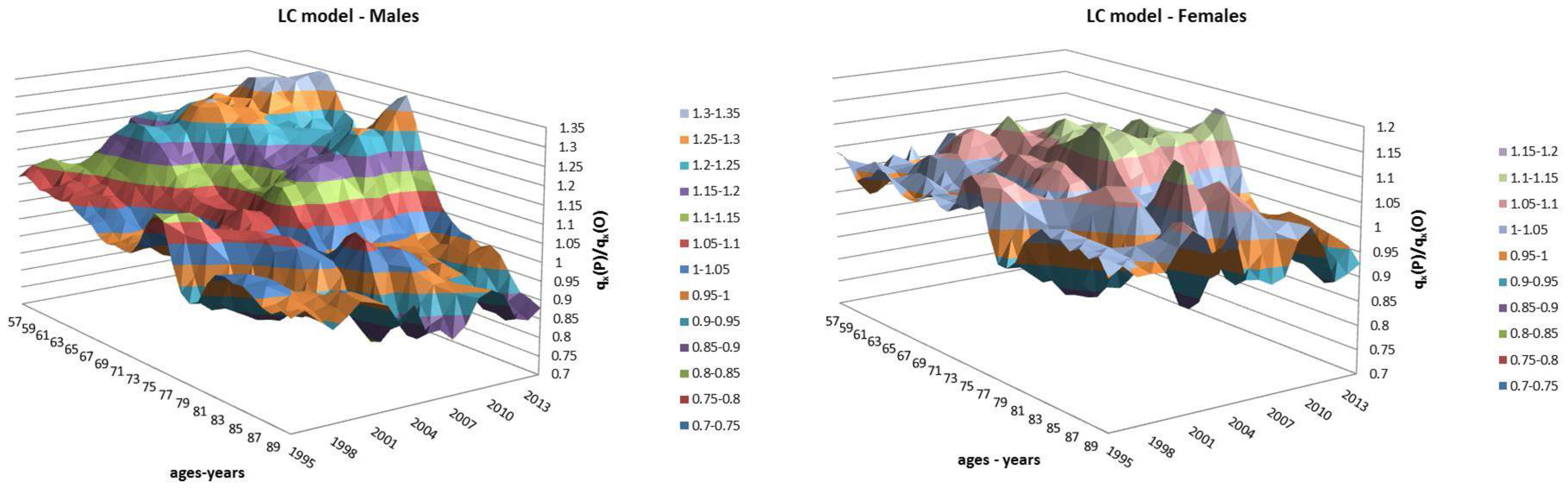
12
For this reason, we decided to plot exclusively the β x dynamics, since they show a more interesting variability with respect to the k t parameters that, in this case, are barely distant parallel and smooth curves among backtest jumps.
13
The choice for the year 2014 was motivated by the observed regular mortality path. The 2015 mortality trend is expected to be increased, particularly at old ages (Istat 2016).
14
These represent the initial years of the 20-year-long database; i.e., 1975 refers to the estimation period 1975–1994, and so on.
15
Equation (A3) has no explicit solution, so it has to be solved numerically.
16
We used MATLAB (R2010b, The MathWorks, Inc., Natick, Massachusetts 01760 USA) for estimation and forecast.
17
We used MATLAB for estimation and forecast.
Figure 1. Italian life tables 1975–2014: males and females entropy ( t H K , ξ ).
Risks 05 00034 g001
Figure 2. Kullback–Leibler divergence with respect to Z ξ at selected ages.
Risks 05 00034 g002
Figure 3. Proportion of temporal variance explained by the models: 1975–1994.
Risks 05 00034 g003
Figure 4. Residuals q x , t O q x , t P by age x: 1975–1994.
Risks 05 00034 g004
Figure 5. LC and CBD models: comparisons between observed and forecast mortality trends.
Risks 05 00034 g005
Figure 6. Lee–Carter Fixed Horizon Backtest: q x , t P q x , t O ratio.
Risks 05 00034 g006
Figure 7. LC Fixed Horizon Backtest forecast: comparison between observed death rates and the corresponding 95% confidence interval of the forecast based on the time series 1975–1994.
Risks 05 00034 g007
Figure 8. Cairns–Blake–Dowd Fixed Horizon Backtest: q x , t P q x , t O ratio.
Risks 05 00034 g008
Figure 9. CBD Fixed Horizon Backtest forecast: comparison between observed death rates and the corresponding 95% confidence interval of the forecast based on the time series 1975–1994.
Risks 05 00034 g009
Figure 10. Fixed Horizon Backtest forecast: comparison between CBD and LC confidence intervals at age 85.
Risks 05 00034 g010
Figure 11. LC Jumping Fixed-Length-Horizon: β x parameter estimates.
Risks 05 00034 g011
Figure 12. LC and CBD q x , t P q x , t O ratio: comparison between models. Note: the curves represent the average of the q x , t P q x , t O ratio over the five-years forecast horizon.
Risks 05 00034 g012
Figure 13. CBD Jumping Fixed-Length-Horizon: parameter estimates.
Risks 05 00034 g013
Figure 14. LC and CBD q x , t P q x , t O ratio: comparison between models on the same gender. Note: the curves represent the average of the q x , t P q x , t O ratio over the five-years forecast horizon.
Risks 05 00034 g014
Figure 15. LC Rolling Fixed-Length Horizon Backtests: q x , t P q x , t O ratio 2014.
Risks 05 00034 g015
Figure 16. CBD Rolling Fixed-Length Horizon Backtests: q x , t P q x , t O ratio 2014.
Risks 05 00034 g016
Figure 17. CBD Rolling Fixed-Length Horizon Backtests (age 65): convergence to real data (2014).
Risks 05 00034 g017
Figure 18. CBD Rolling Fixed-Length Horizon Backtests (age 85): convergence to real data (2014).
Risks 05 00034 g018
Figure 19. LC Rolling Fixed-Length Horizon Backtests (age 65): convergence to real data (2014).
Risks 05 00034 g019
Figure 20. LC Rolling Fixed-Length Horizon Backtests (age 85): convergence to real data (2014).
Risks 05 00034 g020
Table 1. Proportion of persons aged 30 and expected to be alive at selected ages.
Italian Period Life Tables
Ages197519801985199019952000200520102014
Male
500.94380.94830.95540.95830.95910.96620.97220.97550.9777
600.84060.84870.86460.88390.89510.909620.92420.93240.9376
700.62920.64090.66910.70810.73510.77320.80600.82570.8385
800.30140.31610.35390.40290.44060.49360.54340.59120.6188
900.04640.05270.06820.09540.11700.13960.16480.19960.2250
950.00800.00960.01400.02350.03180.04010.04910.05950.0743
Female
500.97030.97390.97690.97850.97960.98220.98500.98650.9871
600.91940.92900.93640.94270.94730.95250.95850.96200.9639
700.80090.81680.83370.85460.86810.88280.89720.90530.9087
800.50700.54030.58140.62490.65760.695610.73220.75400.7674
900.11540.14330.16290.21410.25470.28600.32970.36530.3878
950.02260.03260.03800.06260.08300.10300.12590.14200.1654
Table 2. Jumping fixed-length horizon backtests data horizon.
Lookback HorizonLookforward Horizon
1975–19941995–1999
1980–19992000–2004
1985–20042005–2009
1990–20092010–2014
Table 3. Rolling fixed-length horizon backtests data horizon.
LookbackLookforwardLookbackLookforward
1975–19941995–2014 (20)1985–2004 2005-2014 (10)
1976–19951996–2014 (19)1986–20052006–2014 (9)
1977–19961997–2014 (18)1987–20062007–2014 (8)
1978–19971998–2014 (17)1988–20072008–2014 (7)
1979–19981999–2014 (16)1989–20082009–2014 (6)
1980–19992000–2014 (15)1990–20092010–2014 (5)
1981–20002001–2014 (14)1991–20102011–2014 (4)
1982–20012002–2014 (13)1992–20112012–2014 (3)
1983–20022003–2014 (12)1993–20122013–2014 (2)
1984–20032004–2014 (11)
Table 4. Root Mean Squared Errors (RMSE) between observed q x , t O and forecast q x , t P .
Fixed Horizon Backtest
CBD modelLC model
Prediction YearsMaleFemaleMaleFemale
1995-20140.006250.004010.005960.00274
Jumping Fixed-Length Horizon Backtests
CBD modelLC model
Prediction YearsMaleFemaleMaleFemale
1995–19990.003210.002010.003860.00210
2000–20040.004700.004110.005320.00369
2005–20090.003730.003660.004550.00301
2010–20140.002500.002290.002990.00219

