1. Introduction
Reinsurance is a transaction whereby one insurance company (the reinsurer) agrees to indemnify another insurance company (the reinsured, cedent or primary company) against all or part of the loss that the latter sustains under a policy or policies that it has issued. For this service, the ceding company pays the reinsurer a premium, and there are many premium calculation principles (e.g., [
1,
2]; see also [
3,
4]).
Mathematically, let X be the loss for an insurer from a policy or a group of policies. Assume that under a reinsurance treaty, a reinsurer covers the ceded part of the loss, say , where , for a premium . The primary insurer’s retained loss is denoted by . Commonly-used forms of reinsurance treaties are the excess-of-loss treaty, where with deductible level (attaching point) ; and the quota-share treaty, where with a constant (share) .
Optimal forms of reinsurance have been studied extensively in the literature. Most of the results obtained are from the cedent’s point of view. That is, the question asked is: for a given premium principle, what is the optimal functional form and/or parameter values of the ceded function
f, such that the cedent’s expected utility is maximized or its risk minimized? For example, by maximizing the cedent’s expected utility, Arrow [
5] concluded that “given a range of alternative possible reinsurance contracts, the reinsured would prefer a policy offering complete coverage beyond a deductible.” Borch [
6] showed that for a fixed premium and expected reinsurance payments, the variance of the cedent’s losses is minimized by the excess-of-loss reinsurance policy. In recent years, various solutions to the optimal reinsurance problem have been obtained where the value-at-risk (VaR) and the tail-value-at-risk (TVaR) have been used to measure the cedent’s risk level (e.g., [
7,
8,
9,
10,
11,
12,
13] and the references therein).
Borch [
14] argues that “there are two parties to a reinsurance contract, and that an arrangement which is very attractive to one party may be quite unacceptable to the other.” However, as pointed out by [
15], optimal forms of ceded functions considering both the cedent and the reinsurer had scarcely been discussed until quite recently. For example, Ignatov et al. [
16] study the optimal reinsurance contracts under which the finite horizon joint survival probability of the two parties is maximized. Kaishev and Dimitrova [
17] derive explicit expressions for the probability of joint survival up to a finite time of the cedent and the reinsurer, under an excess of loss reinsurance contract with a limiting and a retention level. Golubin [
18] studies the problem of designing the Pareto-optimal reinsurance policy by maximizing a weighted average of the expected utility of the insurer and the reinsurer. Dimitrova and Kaishev [
19] introduce an efficient frontier type approach to setting the limiting and the retention levels, based on the probability of joint survival. Cai et al. [
20] analyse the optimal reinsurance policies that maximize the joint survival probability and the joint profitable probability of the two parties and derive sufficient conditions for optimal reinsurance contracts within a wide class of reinsurance policies and under a general reinsurance premium principle. Using the results of [
20], Fang and Qu [
21] derive optimal retentions of combined quota-share and excess-of-loss reinsurance that maximize the joint survival probability of the two parties. Cai et al. [
22] study the optimal forms of reinsurance policies that minimize the convex combination of the
s of the cedent and the reinsurer under two types of constraints that describe the interests of the two parties. For the determination of the optimal excess of loss contract considering the dependency between the losses of the insurer and the reinsurer, we refer to [
23] and the references therein.
A closely-related problem to optimal reinsurance is the so-called optimal transfer of risks among partners, where everybody’s interests are considered simultaneously. The usual approach is to identify Pareto-optimal treaties, whereby no agent can be made better off without making another agent worse off. For results in this area, we refer to, e.g., [
6,
7,
24,
25] and the references therein.
In this paper, we determine Pareto-optimal reinsurance policies under which one party’s risk, measured by its VaR, cannot be reduced without increasing that of the other party in the reinsurance contract. We consider two classes of ceded functions:
and:
Note the inclusion
, which has been verified by [
13]. Furthermore, for every
both
f and
are Lipschitz continuous, and they are comonotonic.
The requirements that the ceded function
f is non-decreasing and that the bounds
hold for all
x are needed in
and
to avoid the moral hazard problem in reinsurance. The additional requirement of the convexity of
f in
essentially requires that
approaches infinity linearly when
and thus disallows the popular layered reinsurance policies. Nevertheless, this class includes the important quota-share and the excess-of-loss reinsurance policies. Note also that both classes are of interest in the more general context of economic theory with two agents having conflicting interests. Optimal reinsurance problems with admissible classes
and
have been studied extensively in the literature, and we refer to [
13] for an informative review.
For simplicity of discussion, we assume that the reinsurance premiums are determined by the expected premium principle:
where
is the safety loading. Hence, the cedent’s total loss becomes:
and the reinsurer’s total loss under the reinsurance contract is:
In this paper, we use VaR to measure the insurer’s and reinsurer’s risk level. A natural starting point for measuring the (joint) risk of the cedent and the reinsurer is a bivariate risk measure, such as the bivariate
([
26]) of the pair
and
. However, since the ceded loss
and the retained loss
are comonotonic (see [
27,
28] for a very detailed discussion of the concept of comonotonicity with applications), the set of values of the bivariate
s of
and
is determined by values of the univariate
of
and
. Therefore, the Pareto-optimal reinsurance policies could be determined by minimizing a linear combination of the univariate
s of
and
. We note in this regard that the optimization criterion of minimizing linear combinations of the risks of the cedent and the reinsurer was adopted by [
7,
22]. Our arguments provide an additional economic meaning to such criteria.
Although VaR is not sub-additive in general, it was shown that it is sub-additive in the deep right tail in many cases of interest (e.g., [
29]). General results related to optimal forms of reinsurance (risk exchanges) using the so-called distortion risk measures exist in the literature, and we refer to [
7,
8,
25]. The distortion risk measures are very general and include VaR, TVaR and proportional hazards transforms as special cases. The feature of the current paper is that we extend the geometric approach of [
12] to our optimization problem that considers the interests of the two parties. The geometric proofs facilitate intuition and enable us to avoid lengthy and complex mathematical arguments. We derive closed-form and user-friendly formulas for the optimal reinsurance policies and thus provide a convenient route for practical implementation of our results.
The rest of the paper is organized as follows.
Section 2 provides preliminaries and shows (cf. [
25]) that the form of Pareto-optimal reinsurance policies can be determined by minimizing linear combinations of the cedent’s and the reinsurer’s risks. In
Section 3 and
Section 4, we determine optimal reinsurance forms and derive the corresponding optimal parameters when the feasible classes of ceded functions are
and
, respectively. There, we also provide illustrative numerical examples.
Section 5 provides further insights regarding the results of our numerical examples.
Section 6 concludes the paper.
2. Preliminaries
Let
and
denote the cumulative distribution function (c.d.f.) and the survival function of
X, respectively. Furthermore, let
and
denote the c.d.f.’s of
and
, respectively. Then, the individual
s of the cedent and the reinsurer under the reinsurance contract are:
and:
respectively. To consider the risk of both the cedent and the reinsurer, we propose to use the bivariate lower orthant
introduced by [
26], which is:
For any ceded function
, the random variables
and
are comonotonic, and so:
Therefore, when the “joint” risk of the cedent and the reinsurer is measured by their bivariate lower orthant VaR, one could work with the marginal VaRs of and , instead of the much more complicated joint VaR.
In the following, we assume that the probability levels in the VaRs used by the cedent and the reinsurer are possibly different, say
and
, respectively, and then determine the Pareto-optimal reinsurance policies (ceded functions
f) in the sense that one party’s risk, measured by its VaR, cannot be reduced without increasing the other party’s VaR. Mathematically, let
denote a ceded function in an admissible set
, such as
or
. Let the corresponding cedent’s and reinsurer’s total losses under the ceded function
be denoted by
and
, respectively. Then,
is a Pareto-optimal reinsurance policy if there is no ceded function
belonging to the admissible set
, such that:
and:
with at least one of the inequalities being strict. To find the Pareto-optimal reinsurance policies, we utilize the following proposition.
Proposition 1. All Pareto-optimal reinsurance policies f in , , can be determined by solving the problem:where . Proof. Similar to the discussion on page 90 of [
30], one method to find Pareto-optimal decisions is to choose two positive constants
and find:
Without loss of generality, we set
and
with
. In more detail, let
g be a function belonging to
and minimizing (
2), then there cannot exist in
any function
such that
and
with at least one of the inequalities being strict, because otherwise, we would have:
This is a contradiction to the assumed property of function g.
Furthermore, for any two ceded functions
, the family
of ceded functions defined by
is a subset of
and satisfies:
and:
Equation (
3) is satisfied because:
where the last equality is due to the fact that
and
are non-decreasing functions of the same random variable
X and therefore comonotonic. Similarly, Equation (
4) is satisfied. Therefore, Condition C on page 90 of [
30] is satisfied, and we conclude that all Pareto-optimal reinsurance policies in
can be found by solving Problem (
2). ☐
In view of Proposition 1, throughout the rest of this paper, we seek optimal reinsurance policies by solving the optimization problem:
for
, which is equivalent to minimizing:
As shown by [
13], we have
, and every function
is Lipschitz-continuous and, hence, continuous. Consequently (e.g., [
27]), for every
, we have
and thus, with
and
, the optimization problem becomes:
Since we allow
, the relationships between the probability levels
and
, as well as
need to be discussed. Namely, we have the following observations:
If
and
, then
. Thus,
when
, the solution to Problem (
6) is
for all
x;
when , the solution is ;
when , the objective function is always zero.
If
and
, then
and
. Thus,
when , the optimal ceded function is ;
when
, the form of the optimal ceded function is similar to the case when
, with only the risk and the profit of the cedent considered (the solution for the latter case can be found in Case 2 of
Section 3.2 and
Section 4.2 below);
when , the optimal ceded function is .
If
and
, then
and
. Thus,
Throughout the rest of this paper, we only consider the optimal forms of reinsurance policies under the conditions and .
Now, we are ready to determine the optimal forms of
f, the task that makes up the contents of the following two sections. Namely, in
Section 3, we consider the case when the admissible set of ceded functions is
and in
Section 4 when the admissible set is
. As noted earlier, both classes are of interest in the broad context of economic theory, with the class
being more relevant to reinsurance policies. Nevertheless, the class
includes the important quota share and excess-of-loss reinsurance policies that provide natural reference points for analysing the optimal reinsurance policies in
.
4. Optimal Reinsurance Policy When
In this section, we determine optimal reinsurance policies when
, that is when both
f and the retained loss function
are non-decreasing. Comparing this situation with the earlier
, we can now deal with non-convex ceded functions, such as
for any retention level
. Mathematically, the problem becomes:
As pointed out in the Introduction, solutions to similar problems exist in the literature, and we refer to [
7,
8,
25] for details and further references. Our contribution in this paper is to generalize the geometric arguments of [
12] to the situation when the interests of both the cedent and the reinsurer are taken into account, and we do so in such a way that allows us to avoid lengthy mathematical arguments and consequently helps us to gain useful intuition. In addition, for all scenarios considered, we are able to provide explicit recipes for determining optimal reinsurance policies.
In
Section 4.1 below, we derive optimal forms of ceded functions, and in
Section 4.2, we determine parameter values of the optimal functions.
Section 4.3 contains an illustrative numerical example, which is a continuation of that of
Section 3.3. Throughout the rest of this section, we assume
and
.
4.1. Functional Form of the Ceded Function
We have subdivided our considerations into three cases.
4.1.1. Case 1:
Similarly to Case 1 of
Section 3.1.1, we determine the functional form of the ceded function
in the following manner. For any
, we seek
, such that
and:
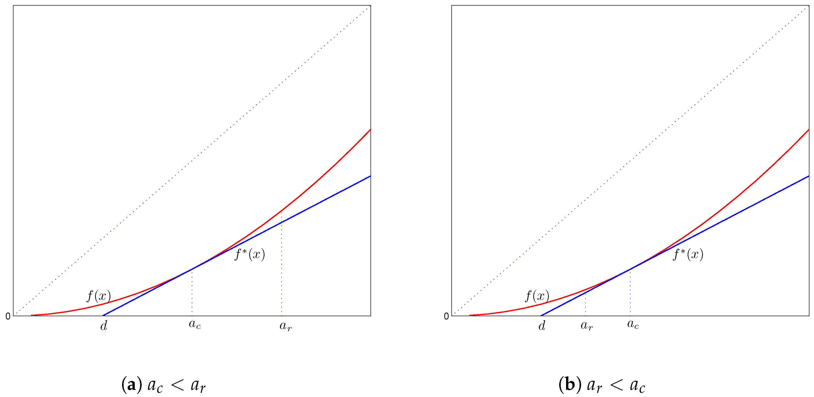
This requires , as well as the entire function to be as small as possible for a fixed value of .
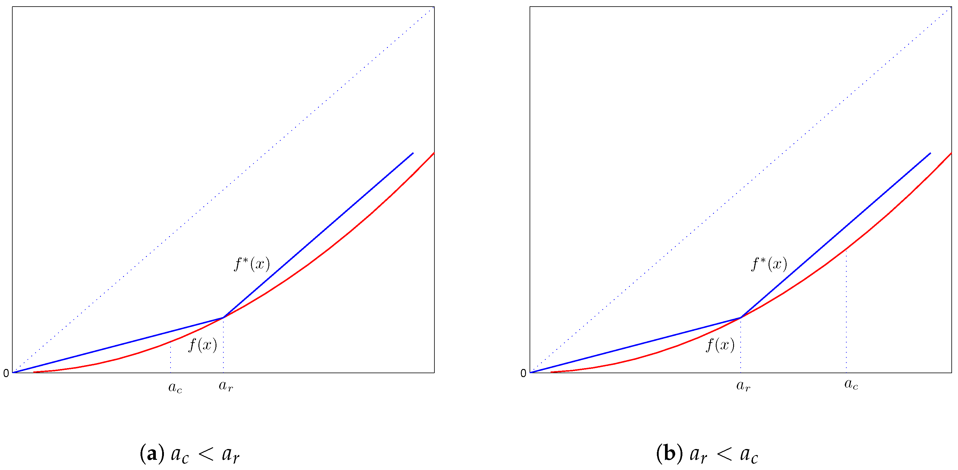
As we see from
Figure 3, because
f is non-decreasing with a slope not exceeding one, the aforementioned requirements are satisfied by the function:
where
can be any constant. The optimal value of
d will be determined in
Section 4.2 below. In reinsurance jargon, the above specified optimal form of the reinsurance policy is for the reinsurer to provide coverage over the layer
.
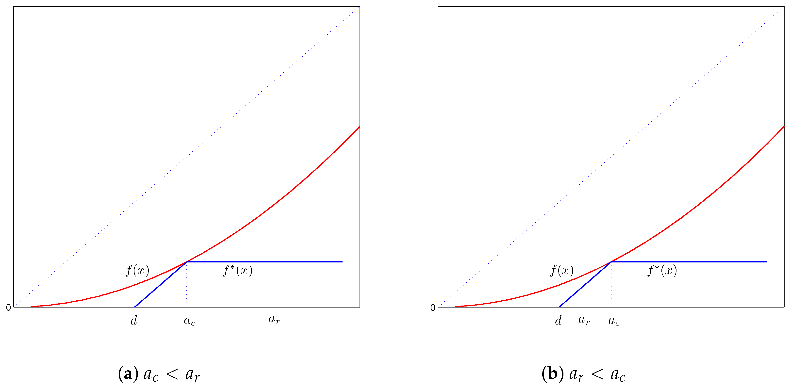
4.1.2. Case 2:
Similarly to Case 2 of
Section 3.1.1, since the coefficients in front of
and
in objective Function (
15) are negative, the optimal reinsurance policy is found by seeking
, such that
and:
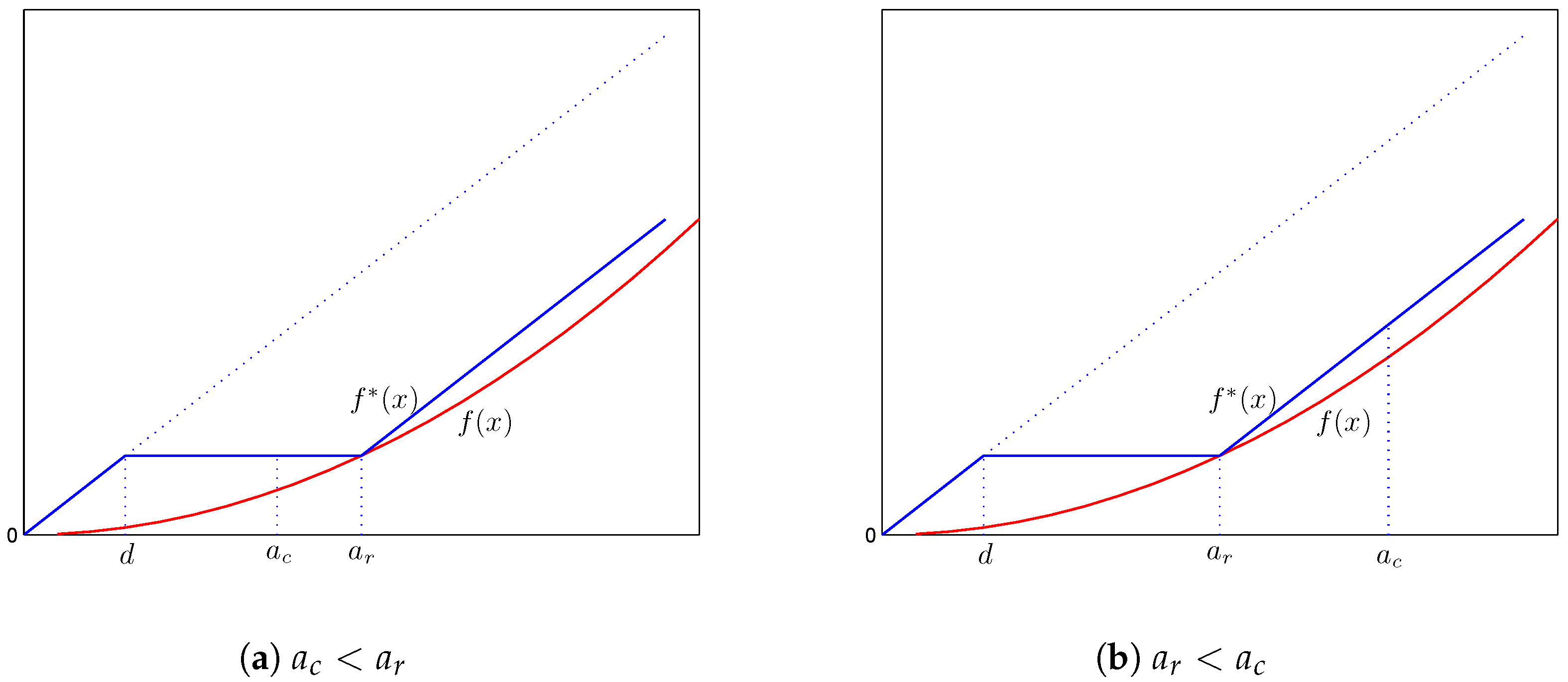
As we see from
Figure 4, these requirements are satisfied by the function:
where
can be any constant. Hence, the optimal form of the reinsurance policy is for the reinsurer to provide a coverage except for the layer
. In other words, the insurer retains losses in the layer
.
4.1.3. Case 3:
In this case, the minimization problem (
15) simplifies to:
When , because the ceded function is non-decreasing, this requires to be constant on the interval . Therefore, any function in with on , where is a constant, is Pareto-optimal.
When , because the slope of the ceded function cannot exceed one, the function increases at the rate of one on the interval . Therefore, any function in with on is Pareto-optimal.
Finally, when , then the objective function is always constant.
4.2. Parameter Values of the Optimal Ceded Function
In this section, we obtain parameter values of the optimal ceded functions that we derived in
Section 4.1. Four cases are considered separately.
4.2.1. Case 1: and
Theorem 5. Under the conditions and , the optimal ceded function is with the parameter:- 1.
when ;
- 2.
when .
In addition, when , then for all x.
Proof. With the function
given by Equation (
16), optimization Problem (
15) becomes:
where:
The derivative:
is increasing in
d. Therefore, when
, then
is minimized at
. When
, then
is minimized at
. Finally, when
, then
is minimized at
, and so,
. ☐
4.2.2. Case 2: and
With the function
given by Equation (
16), optimization problem (
15) reduces to:
where:
We calculate the derivative:
which is an increasing function in
d, and so, we have the following theorem.
Theorem 6. Under the conditions and , the optimal ceded function is with the parameter:- 1.
when ;
- 2.
when ;
- 3.
when and ;
- 4.
when .
If none of the above conditions are satisfied, then for all x.
Proof. We use similar arguments to those in Theorem 2. We illustrate them here by proving Part (1) only. When , the derivative reaches zero at and then remains positive for . Therefore, reaches its minimum at . With this, we conclude the proof of Theorem 6. ☐
4.2.3. Case 3: and
With the function
given by Equation (
17), optimization Problem (
15) reduces to:
where the objective function is:
Thus:
which leads us to the following theorem, whose proof is similar to that of Theorem 3 and thus omitted.
Theorem 7. Under the conditions and , the optimal ceded function is: with the parameter:- 1.
when ;
- 2.
when ;
- 3.
when and ;
- 4.
when and ;
- 5.
when .
If none of the above conditions are satisfied, then for all x.
4.2.4. Case 4: and
With the function
given by Equation (
17), optimization Problem (
15) reduces to:
where:
Thus,
which gives us the following theorem.
Theorem 8. Under the conditions and , the optimal ceded function is:with the parameter:- 1.
when ;
- 2.
when ;
- 3.
when .
If none of the above conditions are satisfied, then for all x.
4.3. The Illustrative Example Continued
In this subsection, we continue the illustrative example of
Section 3.3, but now assume that the admissible class of ceded functions is
.
4.3.1. Scenario A: and
Applying Theorems 5 and 7, we have:
When
, then:
where
can be any constant.
The values of
versus
are reported in
Table 3.
We have the following observations:
Since the cedent and the reinsurer have more choices when , their VaRs under the optimal reinsurance policy are lower than the corresponding ones under . In particular, the reinsurer’s risk is reduced significantly even when .
For , the reinsurer assumes the “good” risk in the layer , as well as losses greater than . The former layer creates profit, and the latter layer does not contribute to its VaR because the chance of penetration is too small compared with the probability level used in its VaR.
For , the insurer retains the “good” risk in the layer , as well as the losses greater than . The former layer creates profit, and the latter layer does not contribute to its VaR because the chance of penetration is too small compared with the probability level used in its VaR.
4.3.2. Scenario B: and
Applying Theorems 6 and 8, we have:
When
,
where
can be any constant. The values of
versus
are reported in
Table 4.
5. A Numerical Comparison of the Optimal Reinsurance Policies in and
In
Section 3.3 and
Section 4.3, we derived the Pareto-optimal reinsurance policies in
and
, respectively. In this section, we compare the two cases.
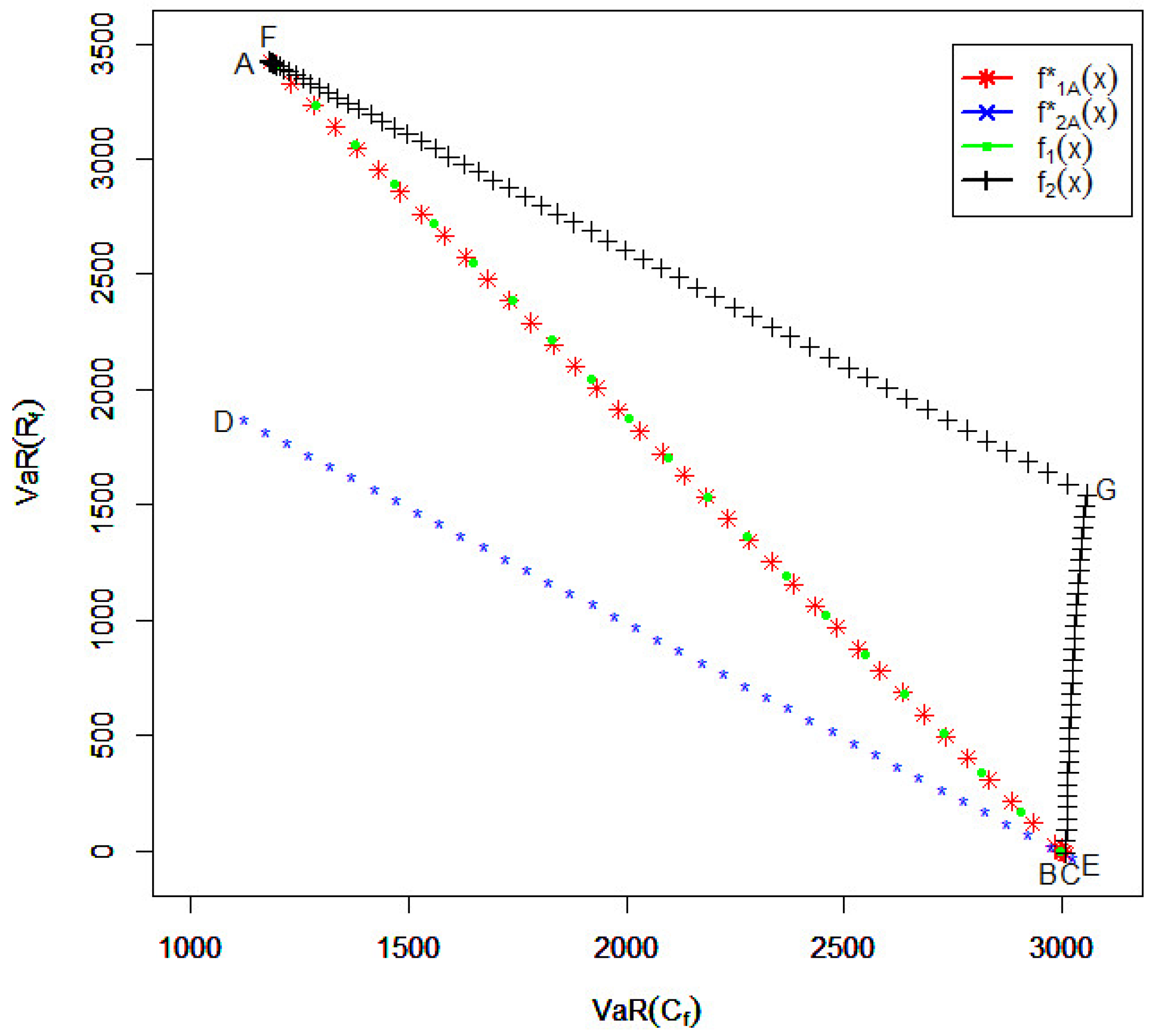
In
Figure 5, we depict
and
obtained for Scenario A with the proportional reinsurance
when
a varies from zero to one and also with the excess-of-loss reinsurance
when the deductible level
d varies from zero to
. The following can be concluded from the figure.
The efficient frontier for the s of the two parties with is represented by the path from to and then to . Note that the points between A and B represent the VaRs of the two parties resulting from the optimal policies obtained with . The points between B and C represent the VaRs of the two parties resulting from the optimal policies obtained with .
The efficient frontier for the VaRs of the two parties when is represented by the path from to .
For the quota-share reinsurance with where a ranges from zero to one, the VaRs of the two parties go from B to . When , the quota-share reinsurance policy is quite close to the efficient frontier.
For the excess-of-loss reinsurance with d ranging from zero to , the VaRs of the two parties go along the path with .
From
Figure 5, we conclude that if the reinsurer worries about the right-hand tail more than the primary insurer (
), then the difference between the efficient frontiers obtained for
and
is significant. This means that the convexity requirement in the definition of
is quite restrictive to the reinsurer, and the coverage with an upper limit (which is not allowed in
) is valuable. In the case when the convexity of the ceded function must be required, quota-share policies are quite efficient.
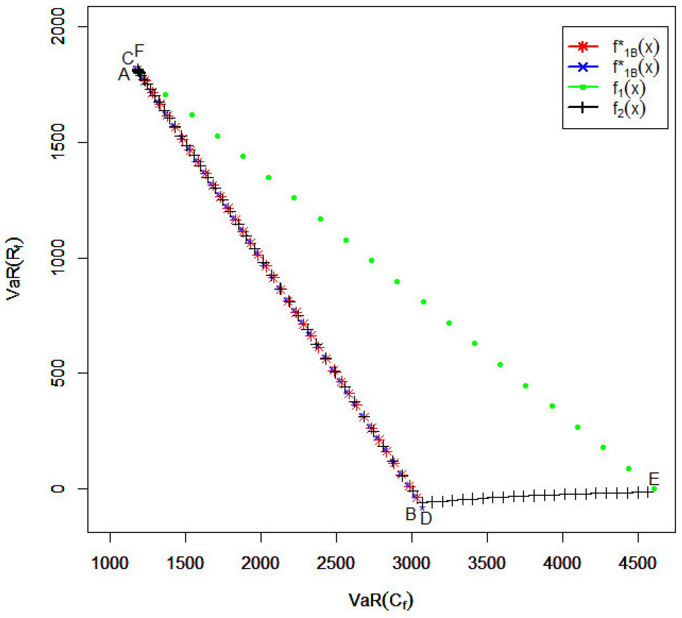
In
Figure 6, we compare
and
obtained for Scenario B with the quota-share reinsurance policies
when
a ranges from zero to one and the excess-of-loss reinsurance policies
when the deductible
d ranges from zero to
.
In particular, we observe the following:
The efficient frontier for the VaRs of the two parties with is represented by the path from to .
The efficient frontier for the VaRs of the two parties when is represented by the path from to . In fact, it can algebraically be shown that the path from B to A is actually a part of the path from D to C. That is, by allowing , the efficient frontier is extended from the path to the path .
For the quota-share reinsurance with the parameter a ranging from zero to one, the VaRs of the two parties are represented by the path from to . We see that when , the quota-share reinsurance policies are not efficient.
For the excess-of-loss reinsurance with the parameter d ranging from zero to , the VaRs of the two parties change along the path . We see that setting is quite efficient, whereas setting is not.
From
Figure 6, we conclude that if the primary insurer worries about the right-hand tail more than the reinsurer (
), then the excess-of-loss policies with the deductible level ranging from
to
provide a good part of the efficient frontier. The quota-share policies are in general inefficient.


