1. Introduction
One of the main issues facing financial and governmental institutions, within the current economic climate, is the forecasting of mortality among an elderly population. Within a vast list of effected parties are public pension policies, private pension funds and life insurance businesses. They face the greatest risk, due to an increasing life expectancy across developed countries.
Over the last few decades it has become widely accepted that mortality can be more accurately measured by the use of stochastic models (see [
1]), since they are better able to capture the uncertainty inherent within the problem. For any given individual, the probability of death naturally increases with age, however, as life expectancy increases over time, we observe improvements in mortality rates. Due to these effects, “dynamic mortality” has been introduced to produce models with age and time dependence. One of the seminal works, which became a benchmark within the industry, is the model of Lee and Carter [
2] who model the central death rate as a two variable function. Since the publication of their work, several extensions of the Lee-Carter model have been proposed. For example, Renshaw-Haberman [
3] considered a model that allows for a cohort effect and Blake and Dowd [
4] proposed a two-factor model for mortality rates. Traditionally mortality models are used for forecasting mortality for older generations (ages over 50) since these mostly affect the uncertainty in the value of financial instruments offered by pension funds due to improvements in mortality and longer life expectancy (phenomena referred to in the literature as
longevity risk). However, Plat [
5] has recently suggested a model that can fit mortality to a wider range of ages (20–89). In [
6] this model has been extended to fit even younger ages (5–89).
A fairly recent stream of actuarial literature has dealt with the phenomenon of stochastic mortality by modelling the instantaneous mortality intensity as a stochastic process. Recent works include Milevsky and Promislow [
7], Dahl [
8], Biffis [
9], Denuit and Devolder [
10], Luciano and Vigna [
11], Shrager [
12]. The mathematical framework in these models has been adapted from the credit risk literature to value securities subject to risk to default. Similarities between the time to default and remaining lifetime and between short-term interest rate and the force of mortality are exploited in this approach. Moreover, if the intensity process is affine, then the survival function for an individual can be derived in a closed form. This is extremely useful when pricing mortality-linked financial products, such as endowments, annuities, variable annuities and other forms of mortality-linked financial securities.
Luciano and Vigna [
11] have studied the applicability of the affine processes, such as Ornstein-Uhlenbeck and Feller, for modelling mortality intensities. The approach is focused on fitting the survival curve for which closed-form solutions are available. The future projections for survival probabilities are made, their closeness to the historical values is discussed, but not evaluated quantitatively.
Another continuous-time mortality model we consider in this work is the one proposed by Wills and Sherris (2011) [
13] for the Australian population. As with the Lee and Carter (1992) [
2] model, it is able to capture the whole “mortality surface” across age and period. Moreover, it takes account of the correlation structure between different generations. This is important for life offices portfolios which often have contracts written on individuals from different cohorts. The authors have shown that the multiple risk factors implied by the model reflect the actual correlation structure between generations inferred from the data and that the model is suitable for pricing financial instruments (see Wills and Sherris [
13,
14]).
The advantages of continuous time mortality models mean that it is important to study how well continuous time processes can predict future mortality. There are numerous papers comparing the performance of mortality models—[
5,
6,
15,
16,
17,
18] are among them. Nevertheless, most of them have focused on discrete stochastic mortality models. For example, Cairns et al. [
15] examined the in-sample fits of eight different discrete time stochastic mortality models. However, as noted in Dowd et al. [
16], it is quite possible for a model to provide a good in-sample fit to historical data and produce forecasts that appear plausible
ex ante, but still produce poor
ex-post forecasts, that is, forecasts that differ significantly from the subsequently realised outcomes. Consequently, a “good” model should produce forecasts that perform well out-of-sample which can be evaluated using backtesting methods.
Lee and Miller [
19] evaluated the performance of the Lee-Carter model by examining the behaviour of forecast errors and plots of “percentile error distributions”, although they did not report any formal test results. In contrast, Dowd et al. [
16] formally evaluate the forecasting performance of six different stochastic mortality models applied to male mortality data for England and Wales. They use a backtesting procedure to test the stability of forecasts over different time horizons and conclude that the investigated models perform adequately, and that there is little difference between them.
The framework for backtesting stochastic mortality models in Dowd et al. [
16] is a very general one. The “backtests” might involve the use of plots whose goodness of fit is interpreted informally, as well as formal statistical tests of predictions. The evaluation can be done for different metrics (the forecasted variable) of interest – possible metrics include mortality rates, life expectancy, future survival rates, the prices of annuities and other life-contingent financial instruments.
This paper focuses on the forecasting performance of several continuous-time models, making a novel contribution to the literature. More specifically, we concentrate on the following continuous-time mortality models: the Ornstein-Uhlenbeck process, the Feller process and the Wills and Sherris model.
To compare the performance of these models to a benchmark, we also include the Lee and Carter model in our experiments. We evaluate the in-sample goodness of fit by using statistical techniques including the BIC criteria and an analysis of the fitted residuals. To assess the forecasting performance of each model we employ out-of-sample back-testing methods using mortality rates as the metric. This is done first by computing the relative error between the forecast and actual mortality rates and then by looking at the percentage of observed mortality rates which fall within a prediction interval. However, the same backtesting procedure using different metrics might be relevant for different purposes.
For our analysis we employ the data of the British and Australian population as they are among the countries where the market for mortality derivatives has started to emerge. According to [
20], the annuity markets are relatively well developed in the UK and US. Some product innovations, such as variable annuities with guaranteed withdrawal lifetime benefits have been introduced in Australia, Japan and Europe. Multiple mortality and longevity derivatives (such as q-forwards, s-forwards, longevity and survivor bonds and swaps) have been suggested in the literature as well, see [
14,
21]. In [
14,
20] the authors study the securitisation of longevity risk for the Australian pension industry. In [
22] natural hedging of longevity risk with application to the UK population is analysed.
This paper is organised as follows: in
Section 2 we present some notation and description of the data that will be used in the subsequent analysis. In
Section 3 we provide an overview of the Lee-Carter model, which we will use as a benchmark for our comparisons.
Section 4 provides the Wills and Sherris model setup.
Section 5 describes time-homogeneous affine processes.
Section 6 calibrates the four models to the UK female dataset and
Section 7 compares the results of this calibration for the four models.
Section 8 discusses the robustness of the simulation results on the male and female datasets for the British and Australian populations.
Section 9 concludes.
2. Notation and Data Description
Throughout the paper we use the following notation. Define
to be the
observed central death rate in year
t for lives initially aged
x as a number of deaths divided by the population exposure:
Here is the average size of the population aged x last birthday during year t and is the number of deaths during year t recorded as age x last birthday at the date of death. The observed central death rate can be calculated directly from the data.
Another measure of mortality is the force of mortality . It is interpreted as the instantaneous death rate at exact time t for individuals aged exactly x at time t. The probability of death between t and for small t is then approximately . Thus, assuming that the force of mortality remains constant over a year: for , we can approximate the force of mortality with the mortality rate .
A typical dataset consists of a number of deaths, , and the corresponding exposures, , over a range of years t and ages x. The data for the UK we use in this study contains the number of deaths and the population exposure. It was taken from the Human Mortality Database (Human Mortality Database. University of California, Berkeley (USA), and Max Planck Institute for Demographic Research (Germany)). We consider female population aged 50–99 (which is relevant to the pension fund industry) during the years 1970–2009.
3. Lee-Carter Model
In this section we describe general characteristics of the famous Lee Carter model [
2] and its estimation process and forecasting technique. Lee-Carter mortality model is used widely in academia, as well as industry. It has been proposed by Lee and Carter in 1992 specifically for US mortality data covering years 1933–1987. However it has been used as a benchmark model to mortality data from many countries and time-periods. It has been shown (see [
23]) that the Lee-Carter model is a special type of multivariate random walk with a drift (RWD), in which the covariance matrix depends on the drift vector. For estimation of the model parameters, principle component analysis (PCA) with a single component is applied to the census data.
Let
denote the log of the mortality rate in an age group
x and time
t for one country. The mortality rate is modelled as follows:
where
is a set of random disturbances and
,
and
are parameters to be estimated:
- –
is the average mortality curve across ages;
- –
is a set of parameters representing the sensitivity of the mortality rate at age x to changes in ;
- –
is a time-varying parameter representing a common risk factor;
- –
is a zero mean Gaussian error .
The parametrisation in (
2) is not unique, since the likelihood function associated with the model above has an infinite number of equivalent maxima, each of which would produce identical forecasts, see Lee and Carter [
2]. In practice, model identification implies imposing constrains. Lee and Carter adopt the constraints
and
.
The constraint
implies that the parameter
is simply the empirical average over time of the age profile in age group
a:
. We can therefore rewrite the model in terms of the mean centered log-mortality rate,
. Thus, we can rewrite Equation (
2) as a multiplicative fixed effects model for the centered age profile:
As a result, we use parameters (with A and T being the total number ages and the total number of years considered) to approximate the elements of the mortality matrix, where each row represents the age of the population and each column represents the year of the observation, with the age-specific parameter which is fixed over time for all x and the time-specific parameter which is fixed over age groups for all t.
The parameters
and
in the model can be found easily using singular value decomposition (SVD) of the matrix of centered age profiles,
, which we denote by
Z. Then the estimate for
is the first column of
B,
(normalised eigenvector of the matrix
) and the estimate for
is
, where
is the first column of the matrix
U (normalised eigenvector of the matrix
) and
is the first element of the diagonal matrix
L (the largest eigenvalue corresponding to the eigenvectors). Typically, for low-mortality populations, the approximation
accounts for more than 90% of the variance of
, see [
23].
To forecast future mortality, Lee and Carter assume that
and
remain constant over time and the time factor
is viewed as a stochastic process. They find that a random walk with drift is the most appropriate model for their data:
where
is known as the drift parameter and its maximum likelihood estimate is simply
, which only depends on the first and last components of the
vector.
We can forecast
at time
with data available up to period
T, as follow:
From this model, we can obtain forecast point estimates, which follow a straight line as a function of
h with slope
:
To make a point estimate forecast for log-mortality we plug the obtained expression for
into the vectorised version of expression (
3):
where
and
are the estimates of
and
respectfully obtained using SVD.
4. Wills and Sherris Model
Wills and Sherris suggested a stochastic longevity model where the force of mortality for age
x at time
t has the following dynamics (see [
13,
14]):
In the above expression the drift parameter is an affine function of the current age
, while volatility function is a constant.Applying the Ito’s lemma, we find the solution to the SDE (
8):
which can be written as follows:
For all ages
, we consider a multivariate random vector of mortality rates:
The dynamics
are assumed to be driven by the multivariate Wiener process
, with mean zero and the instantaneous correlation matrix given by:
This means that the Wiener processes are independent between time periods, but correlated between ages and the multivariate Wiener process can be expressed in terms of independent Wiener process as .
Thus, the model described by Equation (
8), becomes a system of equations where the dependence between the ages is captured by the
term:
Using the fact that the distribution of the changes in the force of mortality follows a normal distribution, we can find the parameters
,
and
by means of maximum likelihood estimation. In particular,
To estimate the covariance matrix of
, we apply Principle Component Analysis (PCA) to the standardised residuals of the model. For each year, they are the realisations of the random vector
:
5. Time-Homogeneous Affine Processes
Mortality intensity since recently has been modelled as a stochastic process, (see Cairns [
1]). In this field, an important stream of literature focuses on describing death arrival as the first jump time of a Poisson process with stochastic intensity. This approach is named doubly stochastic. Milevsky and Promislow [
7] have used a stochastic force of mortality, whose expectation at any future date has a Gompertz specification. Dahl [
8], Biffis [
9], Denuit and Devolder [
10] and Schrager [
12] in modelling the stochastic force of mortality have applied the same mathematical tools used in the credit risk literature to model the time to default. Under this setting, the remaining lifetime of an individual,
, is a doubly stochastic stopping time with intensity
λ.
Let the mortality process
represent the mortality intensity of an individual belonging to the generation
x at (calendar) time
t and
τ be the time of death of an individual of generation
x. Then the survival probability from time
t to time
is defined as a function of
τ,
, under the probability measure
P, conditional on the survivorship up to time
t:
A doubly stochastic stopping time is the analogue of the first jump time of a Poisson process, where the intensity is a stochastic process. If
τ is the first jump time of a Poisson process with parameter
μ, then
Similarly, if
τ is doubly stochastic with intensity
μ, then the individual’s survival function
is given by
where
describes the information at time s.
In general, the expectation in (
11) is not easy to calculate. However, if the intensity process is affine (see Duffie, Filipovic and Schachermayer [
24]), then it is possible to provide the closed form for the survival probability:
where the functions
and
satisfy generalised Riccati ODEs, which can be solved analytically or at least numerically. The closed-from expression of survival probabilities (
12) in affine framework allows to price financial instruments written on the underlying population, such as endowments, annuities, variable annuities and other forms of mortality-linked financial securities. Due to this result, in applications the processes selected for the mortality intensity are typically affine.
Luciano and Vigna [
11] proposed and tested time-homogeneous non-mean reverting affine processes for the intensity of mortality, which are natural generalisation of the Gompertz law of mortality. They consider Ornstein Uhlenbeck process, Ornstein Uhlenbeck process with jumps and the Feller process. They provide the analytical solutions for survival function (
12) for these processes and discuss the appropriateness of using them in modelling mortality. Calibrations on historical data show that despite their simple form, these processes fit mortality intensity dynamics very well. Another study shows how to use these processes to delta-gamma hedge mortality and interest rate risk, see Luciano, Regis and Vigna [
22] .
5.1. The Ornstein-Uhlenbeck Processes
The SDE for the Ornstein-Uhlenbeck (OU) process without mean-reversion, with the associated solutions of the Riccati ODE
and
, is the following:
where
,
.
We calibrate the parameters of the OU process by means of Maximum Likelihood method applied to the mortality intensities.
Assume that the dynamics of the mortality intensity is described by the OU process without mean reversion as given by SDE (
13). Then, the conditional probability density of an observation
, given a previous observation
(with a
δ time step between them), has a form (here we omit
x which symbolises a certain generation):
where
.
The log-likelihood function of a set of observations
can be derived from the conditional density function:
From the Maximum Likelihood conditions we find the following equations for the parameters:
The OU process in general can produce negative paths. The probability of
turning negative is
where Φ is the distribution function of a standard normal.
In fact, the function
is increasing in
and decreasing in
a, as well as the probability of negative values of
. In mortality modelling applications the probability that
takes negative values is very small, because in practice the obtained value of
is small enough and the value of
a, on the contrary, is high enough. In our calibration we check that the values of the obtained parameters are such that there are no negative intensities. Otherwise, to keep mortality intensity positive, it is possible to impose a restriction using Equation (
16) during the parameter search, such that probability (
16) is negligible (see Luciano and Vigna [
11] for more details).
5.2. The Feller Process
The fourth model is the Feller process which is described by the following SDE with the associated solutions of the Riccati ODEs
and
:
where
,
, the boundary conditions are
and
, and the coefficients are:
The solution to the Equation (
17) has the form:
The Feller process is a type of the Cox, Ingersoll, Ross (1985) process [
25] without mean reversion. It was proposed as a model of a short rate for financial market, referred to as the CIR model. This model is described by the following SDE:
where
is the mean-reversion level. Thus, the model suggests that the
is pulled towards
b at a speed controlled by
a. If condition
holds and
, then the CIR process remains strictly positive, almost surely, and the state (marginal) distribution of the process is steady. The marginal density is gamma-distributed. The maximum likelihood estimation of the parameter vector
is based on the transition density. Given
at time
t the density of
at time
is
where
and
is modified Bessel function of the first kind and of order
q. Then the likelihood function of the time series
with the time between two observations
is
from which the log-likelihood function of the CIR process is derived:
where
and
.
There are two approaches to calibrating affine mortality processes to the historical data. One is to match the survival function (Equation (
12)) using the solutions of the Riccati ODEs for the OU (Equation (
13)) and the Feller (Equation (
17)) processes to the set of observed survival probabilities. Another approach is to maximise the likelihood function of the transition density. In this work we employ the second approach as described in [
26] since both for the OU process and the Feller process the transition density is known in closed-form.
6. Models Calibration
In this section we work with the UK female dataset which describes the mortality in population aged 50–99 for the years 1970–2009. First, we divide the data in two data sets: the estimation data set, containing 30 years of observations, from 1970 until 1999; and the backtesting data set containing the last 10 years of observations, from 2000 till 2009. First we estimate the model parameters on the estimation data set, then we make 10-years predictions of mortality rates and calculate how well the forecast is compared with actual mortality rates for the period 2000–2009.
For the Lee and Carter and the Wills and Sherris models we use the whole surface of mortality to calibrate the models. Then, to compare the performance of the models between each other, we chose 19 generations. To have reliable estimation results and to make the comparison between the models which simulate the whole mortality surface (the Lee Carter and the Wills and Sherris models) and the ones which model each generation separately (the OU and the Feller processes) fairer, we take all possible generations from the data, which satisfy the criteria that the length of the backtesting period would not be less than 10 years. This results in 19 generations—aged 42–60 in the year 1970. We obtain the mortality rates for corresponding generations from the surface by taking the relative diagonal of the matrix. For the OU and the Feller processes, however, we calibrate the parameters for each of the 19 generations separately. We calculate the parameters on the estimation time period (1970–1999) and then use them to make forecasts of mortality for the next 10 years. Thus, we build forecasts for these generations and compute the relative error of prediction, as well as the percentage value of the actual mortality rates which fall within the prediction interval in the test period 2000–2009.
6.1. Calibration of the Lee-Carter Model
First of all, we compute the average of the log mortality
for every age over time period 1970-1999 for the estimation dataset and subtract it in order to obtain mean centered log-mortality rates,
. The average of the log mortality for the whole dataset is shown in
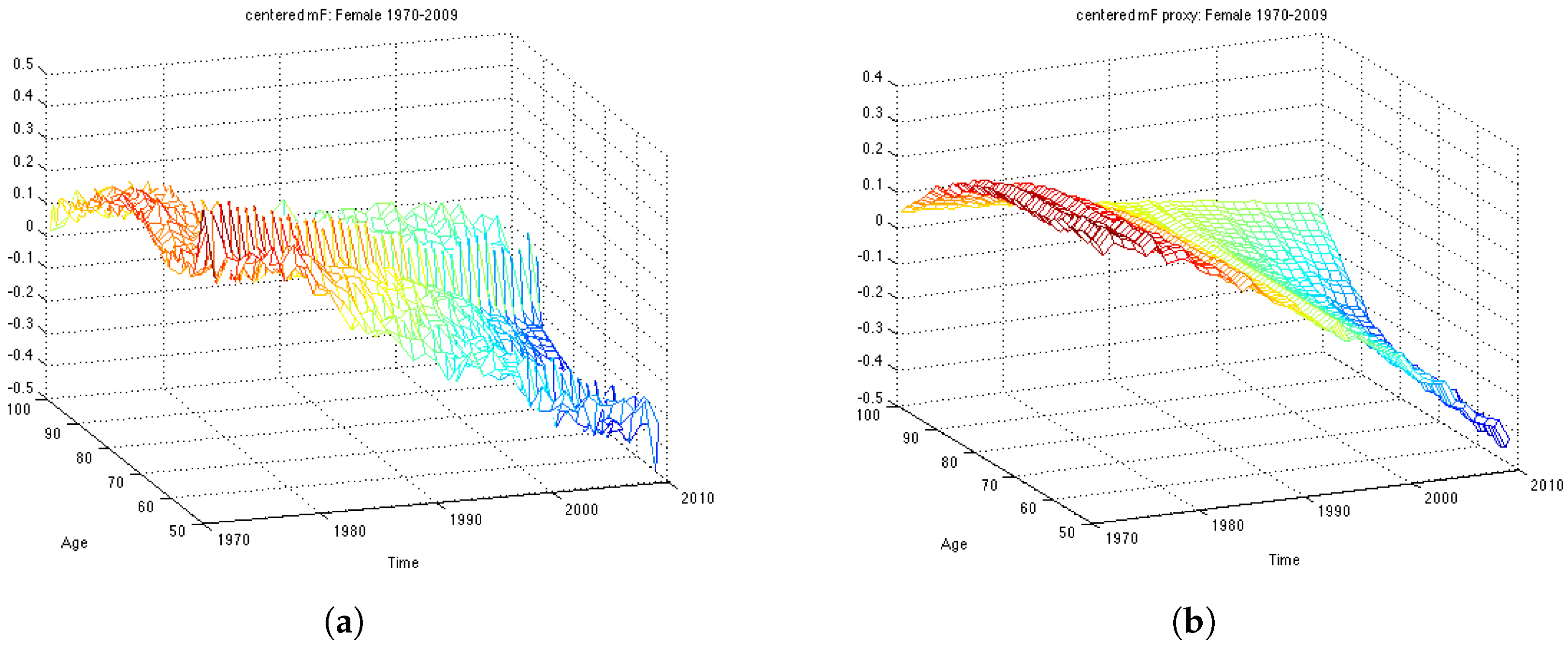
Figure 1. Then, we perform SVD on
matrix and obtain estimates for parameters – two vectors
and
. The actual centered mortality and its SVD approximation are illustrated in
Figure 2.
The obtained ML estimates for the drift and the variance of the innovations are
and
, respectively. Using these parameters we can compute the forecast for
as given by Equation (
4) and its forecast point estimate as described in Equation (
6). In
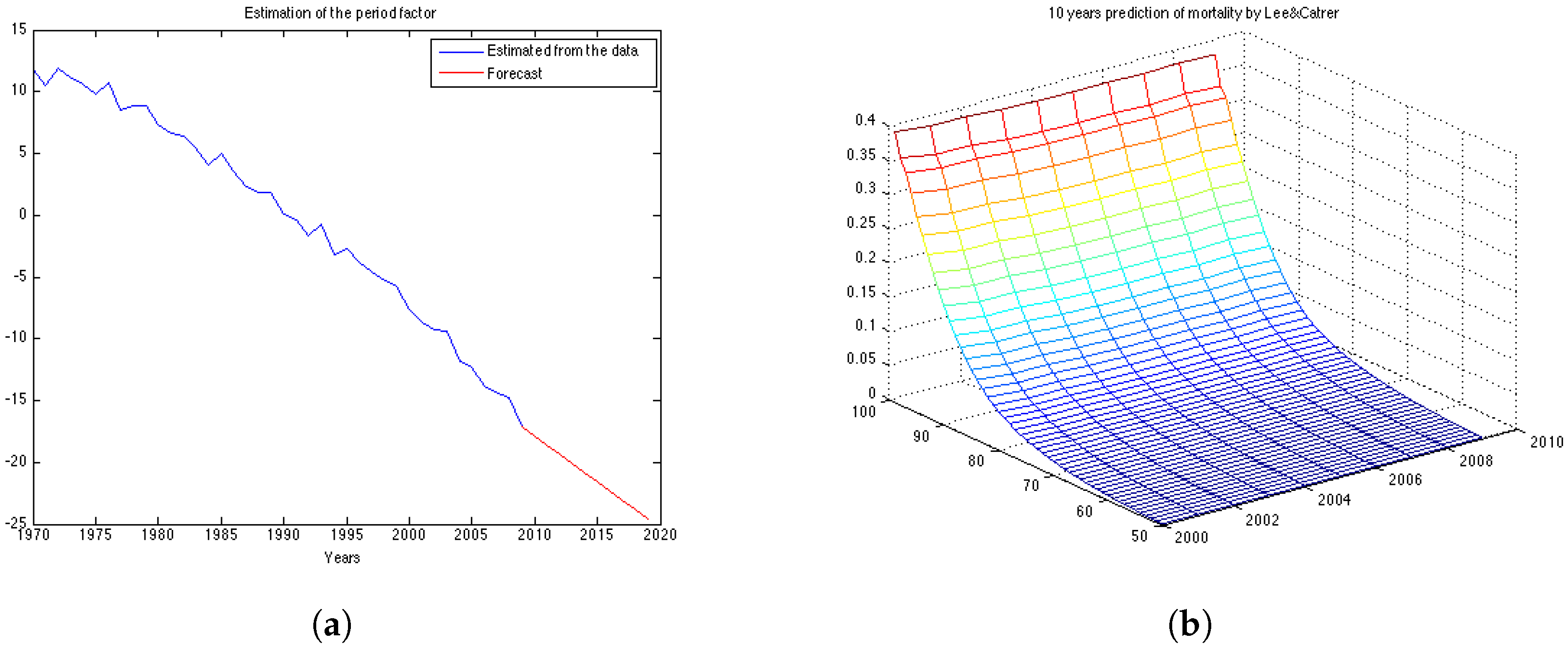
Figure 3a the estimated vector of
and its forecast obtained for the next 10 years (in red) are shown. Then, we calculate the forecast for log-mortality as given in Equation (
7).
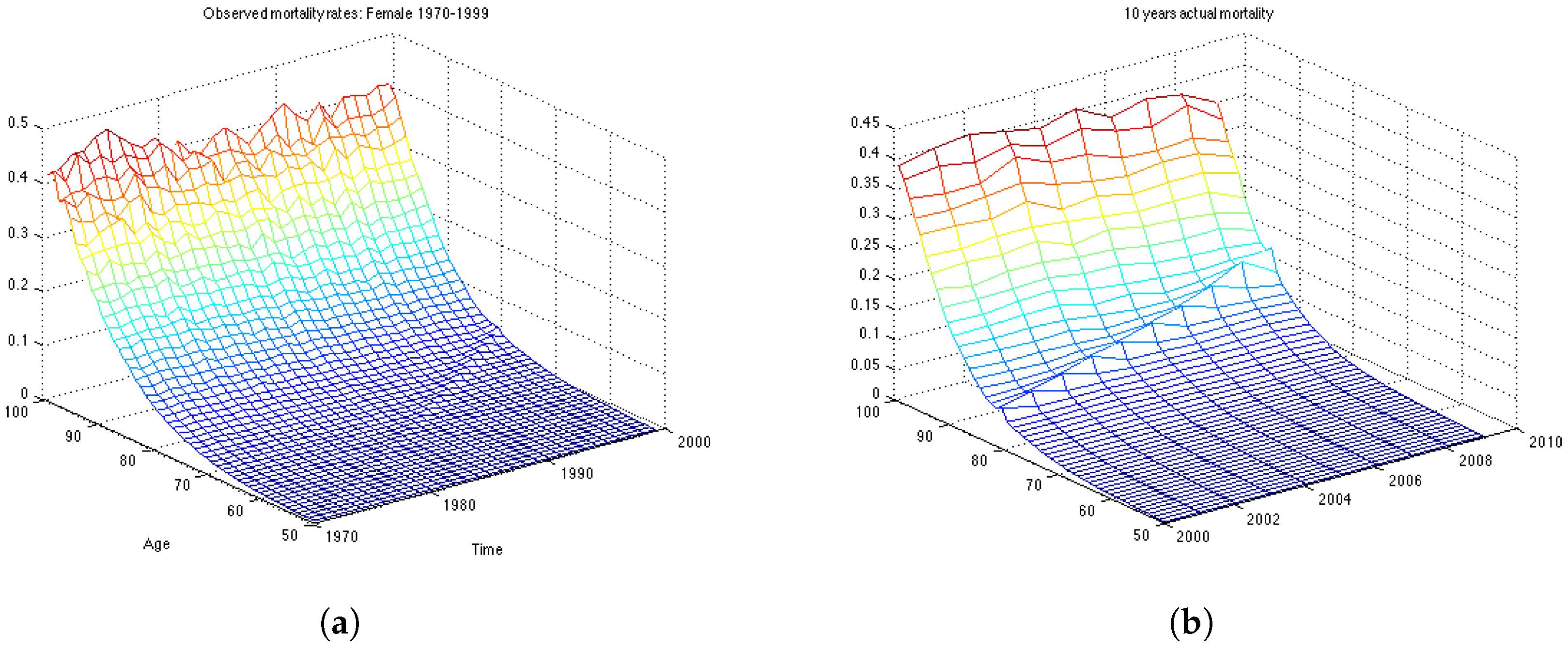
Figure 3b shows the mortality for the 10 years forecasted by the Lee-Carter. The forecast corresponds well to the observed mortality rates for the UK female population presented in
Figure 1b. However, we can see that the cohort effect (diagonal trends in the data present in
Figure 1b) is not captured by the Lee-Carter forecast of mortality.
6.2. Calibration of the Wills and Sherris Model
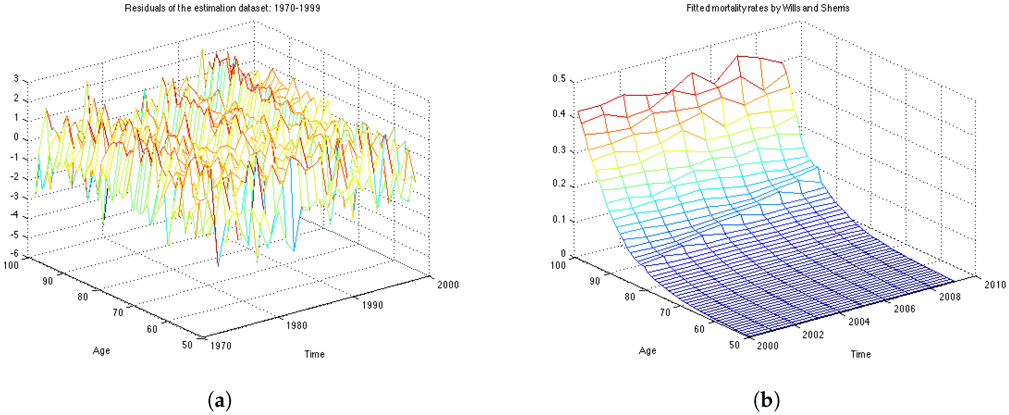
The analysis of the fit is based on the assumption that the residuals are independent and identically distributed normal variables with mean 0 and standard deviation 1.
Figure 4a shows the graph of residuals for the UK female population aged 50–99, years 1970–1999 (the estimation dataset). The plot, together with the residuals descriptive statistics in
Table 1, supports the hypothesis that the residuals follow a standard normal distribution with mean close to zero and standard deviation very close to one. The table also contains the value of the log likelihood function, the BIC criteria and the value of the
χ-square statistics.
The Bayesian information criteria (BIC) is defined as
where:
n – the number of observations (sample size);
k – the number of free parameters to be estimated.
– the maximized value of the likelihood function of the model.
Pearson’s chi-square statistics, defined as
, allows us to evaluate the goodness of fit by testing wether or not an observed frequency distribution differs from the theoretical one. We compare weather the computed value of
with the critical value of the statistic with degree of freedom defined as
The obtained value of the is 1.5835. This is compared to the chi-square distribution with 217 degrees of freedom . Higher values of the statistic suggest a poorer fit. Since the calculated value is very low, the test confirms a very good fit to the data.
To capture the correlation structure between ages we calculate eigenvectors of the matrix of the obtained residuals using Principal Component Analysis.
Table 2 summarises the percentage of the observed variation explained by these vectors. The observed age-correlation matrix has a total of 49 eigenvalues. In our experiments we take first 30 eigenvectors to approximate the correlation matrix as they account for
of the variation.
Figure 4b shows the mortality surface for the test period built with the Wills and Sherris model using the parameters obtained on the estimation dataset. By comparing the forecast with the actual mortality rates (
Figure 1b), we can see that the model gives projections which are similar to the real data, although we see more variation in the simulated mortality intensities. In order to obtain a reliable prediction of mortality rates for a particular generation, we perform Monte Carlo simulations of the mortality surface for the test period and extract from the surface a diagonal corresponding to a specific generation. Then we estimate the mean of the Monte Carlo simulations for a given generation, together with the
prediction interval.
6.3. Calibration of the OU-Process
We calibrate the model on 19 generations and evaluate the goodness of fit by means of the BIC criteria and analysis of the residuals. For each generation x, having a series of length N we use observations (first n years of the sample) to estimate the parameters a and σ and last 10 observation for backtesting the results. For instance, for the UK data, if we consider individuals who were 50 in the year 1970, and we have the data until the year 2009, we have 40 years of observations. Then the first thirty years of observations (1970–1999) is the estimation data and the last ten years of observations (2000–2009) is the backtesting data.
After obtaining the parameters we use the following simulation equation to generate paths of the mortality intensities. This expression is an exact solution of the SDE (
13):
From the mortality intensities one can easily obtain the survival probabilities by means of the analytical formula
12 with
. In this way the expression for a one-year survival curve with
α and
β being constants is:
However, in our study we focus on mortality intensities. We obtain the parameters using the estimation dataset as described above, after which we use them to generate paths and to forecast mortality intensities. Finally, we calculate the error between the forecasted mortality curve and the actual mortality rates.
The residuals of the model are the realisations of the random component
which should follow the standard normal distribution if the parameters are estimated correctly:
We use Kolmogorov-Smirnov statistic to test hypothesis that the errors come from a standard normal distribution.
Taking the mortality intensities for the 7 generations we obtain the parameters presented
In
Table 3 we report the obtained parameters for selected 7 generations. As expected, the
a parameter is increasing with age, which means that the average mortality intensity is larger for older generations. The
σ parameter is also growing with age. This proves the fact that there is more uncertainty in mortality rates for older ages.
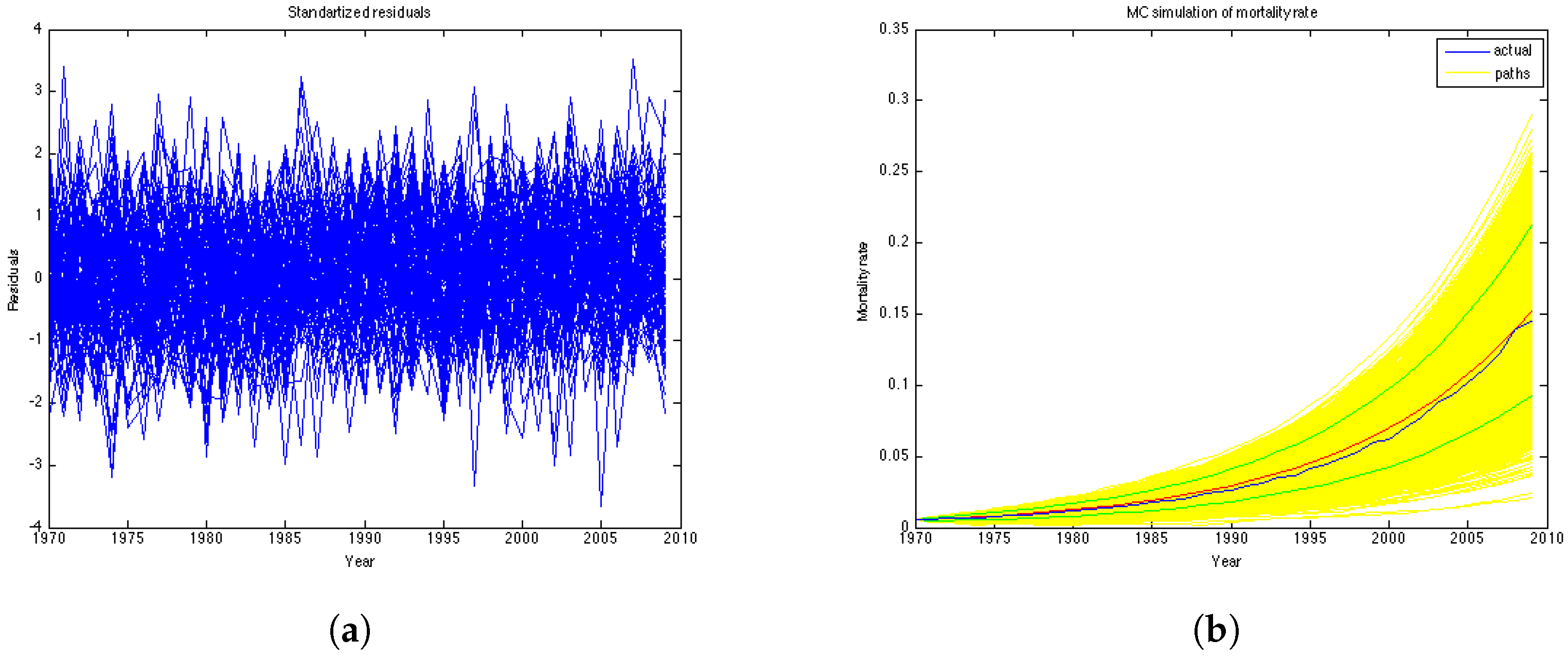
Figure 5a represents the residuals of the model. According to the Kolmogorov-Smirnov test, the errors of the model are confirmed to be standard normal at
significance level.
Figure 5b illustrates historical mortality intensities (in blue), 1000 MC simulations (in yellow), average among simulations (in red) and confidence intervals (in green) for the entire period (1970–2009). This graph is done for the generation aged 51 in the year 1970.
6.4. Calibration of the Feller Process
We have maximised the log-likelihood function as it is stated in Equation (
24) assuming that the mean-reversion parameter is zero.
Table 4 reports the obtained parameters and the value of the maximazed log-likelihood function for each generation. The obtained parameter values correspond well with the previous work, such as in Luciano and Vigna [
11] .
The simulation of the future mortality is performed by discretising Equation (
17) with time step equal to one year:
7. Comparison of the Four Models
To compare the performance of the models for the 19 generations based on their age in 1970. For each, we forecast mortality rates in the period 2000–2009 and compute the relative error of prediction, as well as the percentage of the observed mortality rates in the test period which fall within the prediction interval. The forecast and the prediction bounds are obtained using 15,000 Monte Carlo simulations.
In this section we define the tests of the mean relative error and the prediction intervals. A model can perform very well with respect to the percentage of the mortality rates which fall within the prediction bounds, while at the same time having a high relative error, if its variance grows rapidly and, therefore, the model produces wide prediction bounds. We say that a model is precise if its forecasts of mortality are consistent with respect to the prediction interval and that a model is accurate if its mean absolute forecast errors are small. Of course, it is desirable for a good model to be both accurate and precise. To interpret the results of the experiments, it is important to understand the form of the variance implied by each model which we discuss in this section as well.
7.1. Relative Error
For each
the
relative error is defined as follows:
Since the longevity risk corresponds to lower-than-expected mortality rates, we define the error so that it is positive if the forecast of mortality exceeds the historical values (actual values are lower-than-expected), and negative in the opposite case.
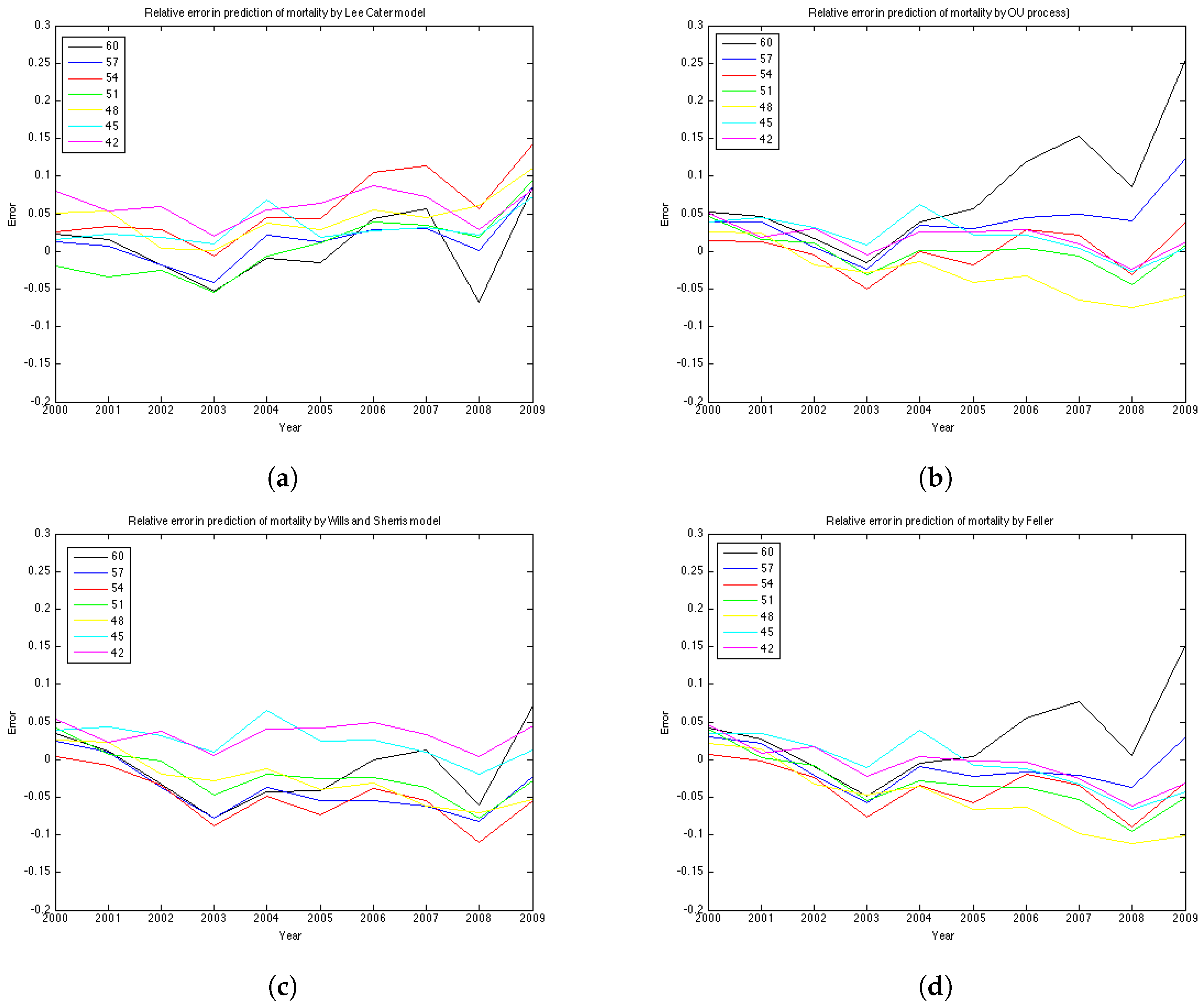
We compute the relative error for 19 generations—they are female aged 42–60 in the base year 1970. Thus, in the test period, for which the graphs of error are plotted, they are 30 years older—72–90 years, respectively.
The results of the experiments are presented in
Figure 6 and
Figure 7 and
Table 5 and
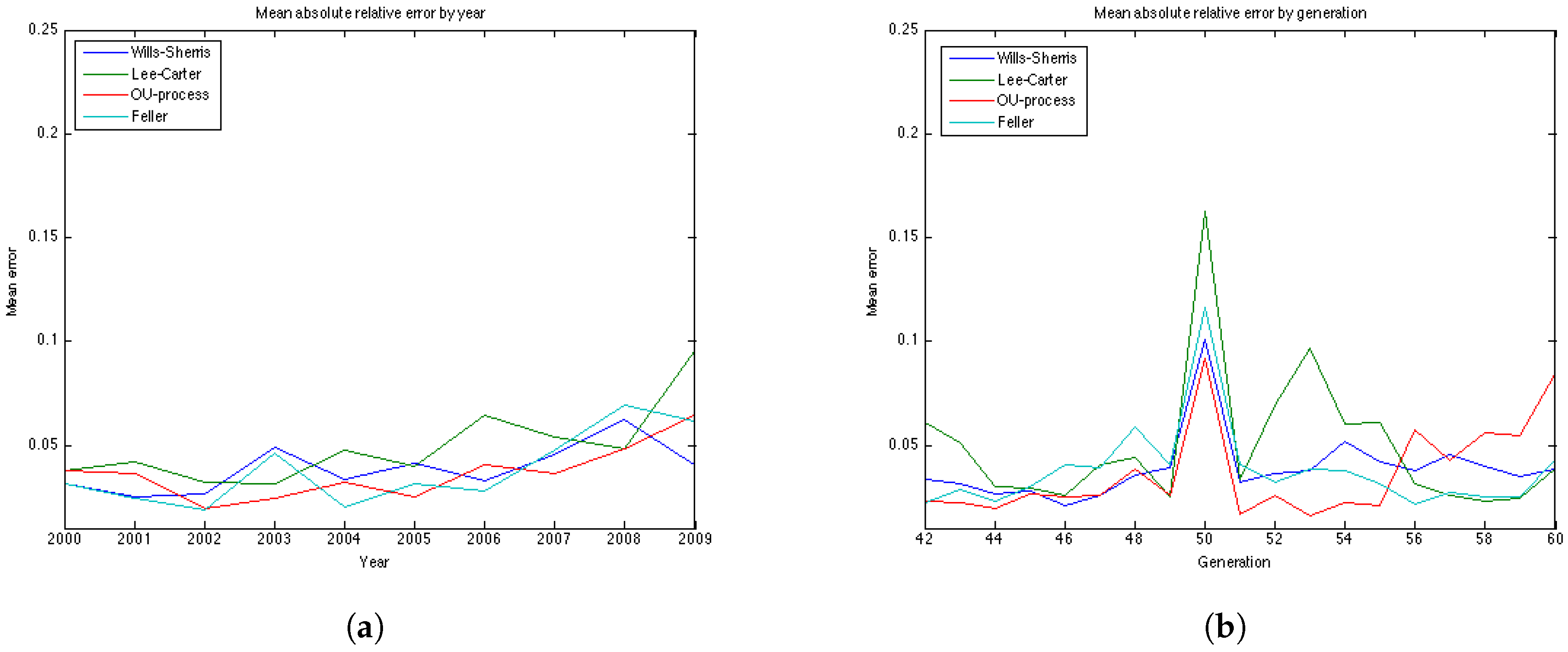
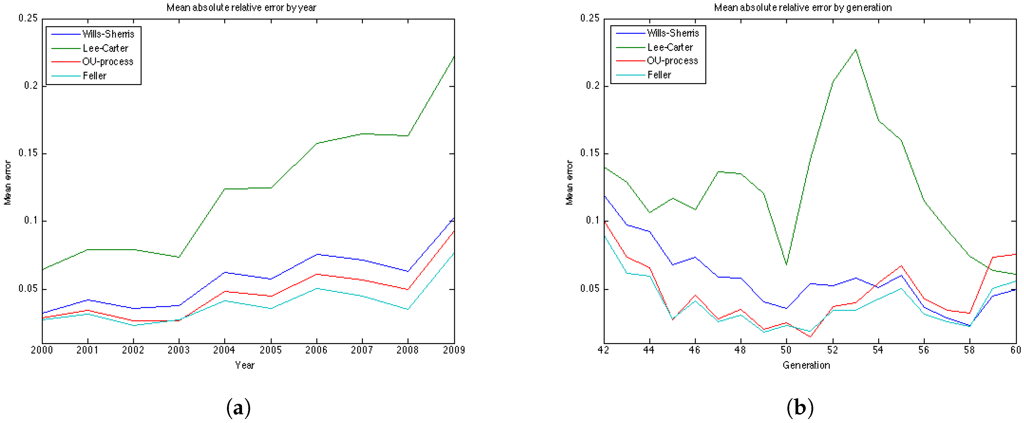
Table 6. The graphs of the mean absolute errors in
Figure 7 illustrate the results shown in
Table 5 and
Table 6. We can see that most of the errors fall in the range
. The exception is the OU process for the generation aged 60 in 1970, especially for later years of projections. The error for this generation in the Feller process forecast is also large – its absolute mean for generation aged 60 in 1970 is 0.0427 (
Table 5). This increases the mean absolute errors for this generation for these processes shown in
Table 5.
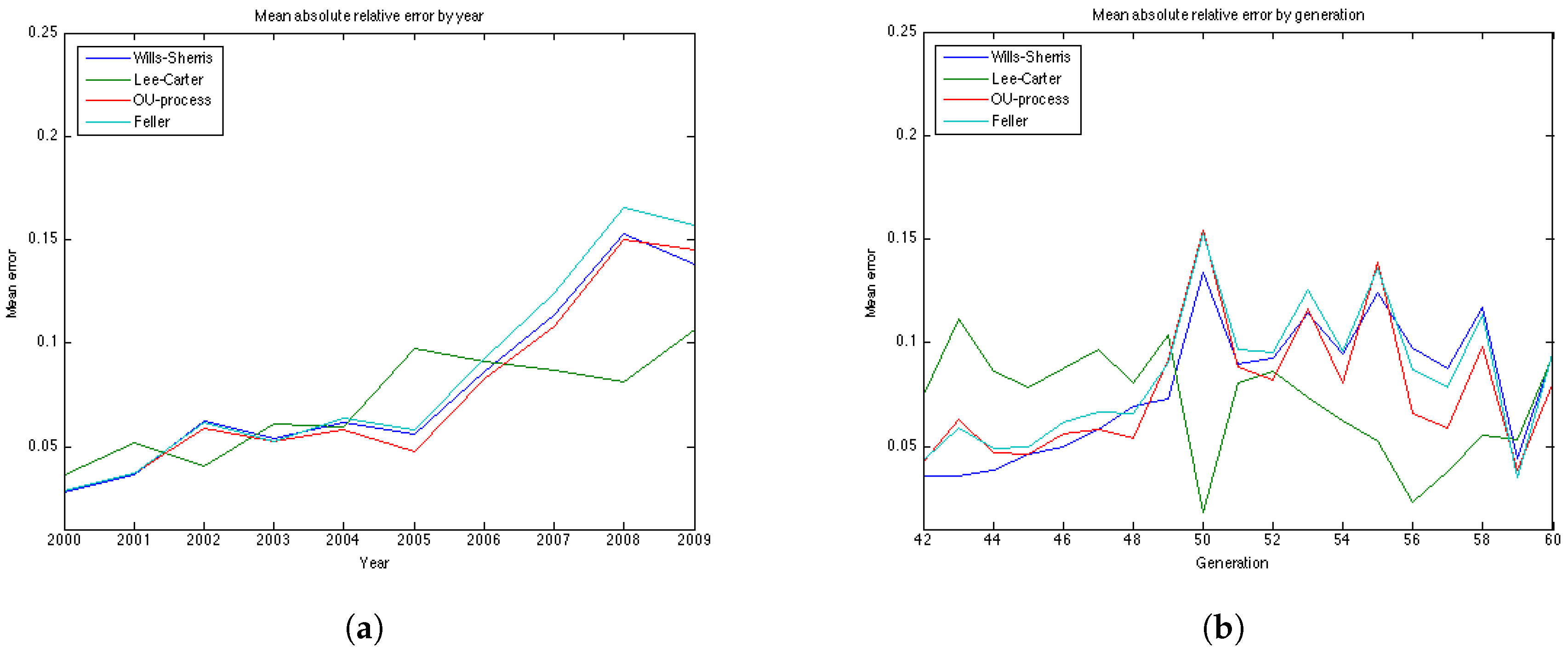
Figure 7b shows the relative absolute error for each year in the test period average over 19 generations. We see that the error is smaller for younger ages . All the models show a high error for the generation aged 50 in the year 1970. This might be due to the cohort effect which is generally present in the UK data. The biggest error for this generation is produced by the Lee-Carter model. The graph of the relative absolute errors averaged over generations by year (
Figure 7a) shows an increasing trend for all 4 models, especially for the Lee and Carter model (red line). This effect is due to the fact that the variances of the projected mortality rates increase with projection time. However, this does not happen at the same rate in different models.
The errors of the Lee-Carter model are mostly positive (
Figure 6a) and we can observe a relative increase of the errors in time for each generation, indicating that the Lee-Carter model has tended to predict mortality rates that are too high. The errors of the Wills and Sherris model exhibit two patterns for different generations (
Figure 6c). They are negative for the older generations (aged 60, 57, 54, 51 and 48 in 1970) and positive for the two youngest ones (45, 42 in 1970). We note that the older generations belong to the lower diagonal of the initial mortality matrix, while the younger two belong – to the upper diagonal of the matrix. Thus, it may be that the Wills and Sherris model has a tendency to overestimate the mortality for younger generations and underestimates the mortality for the older ones.
According to the
Table 5 and
Table 6, the OU process exhibits the lowest mean absolute error, followed by the Feller process, the Wills and Sherris model and the Lee and Carter model for the UK female data.
7.2. Discussion on the Variances
As it has been stated in the description of the model, the variance of the mortality intensity
, conditional on time 0, in the OU specification has a form
, where
t is the time elapsed. For the Feller process, when intensity
is specified by the CIR process of the form:
with
,
,
, the conditional distribution of the mortality intensity at time
t, conditional on time 0 is given by a non-central chi-square distribution:
where
denotes the density of a non-central chi-square random variable with
d degrees of freedom:
and the non-centrality parameter
ν is
The
distribution, has a variance
. Thus, intensity
has a variance:
In the Feller specification, parameter b is not defined and, hence, the number of degrees of freedom d is not defined either. However, we can see that, other parameters being equal, the variance of the OU process should grow faster in time than the variance of the CIR process, as it has term rather than .
The Wills and Sherris model assumes that the distribution of the changes in the force of mortality follows a normal distribution:
Thus, the variance of the mortality intensity grows in time as at each time installment it is multiplied by the mortality rate from the year before.
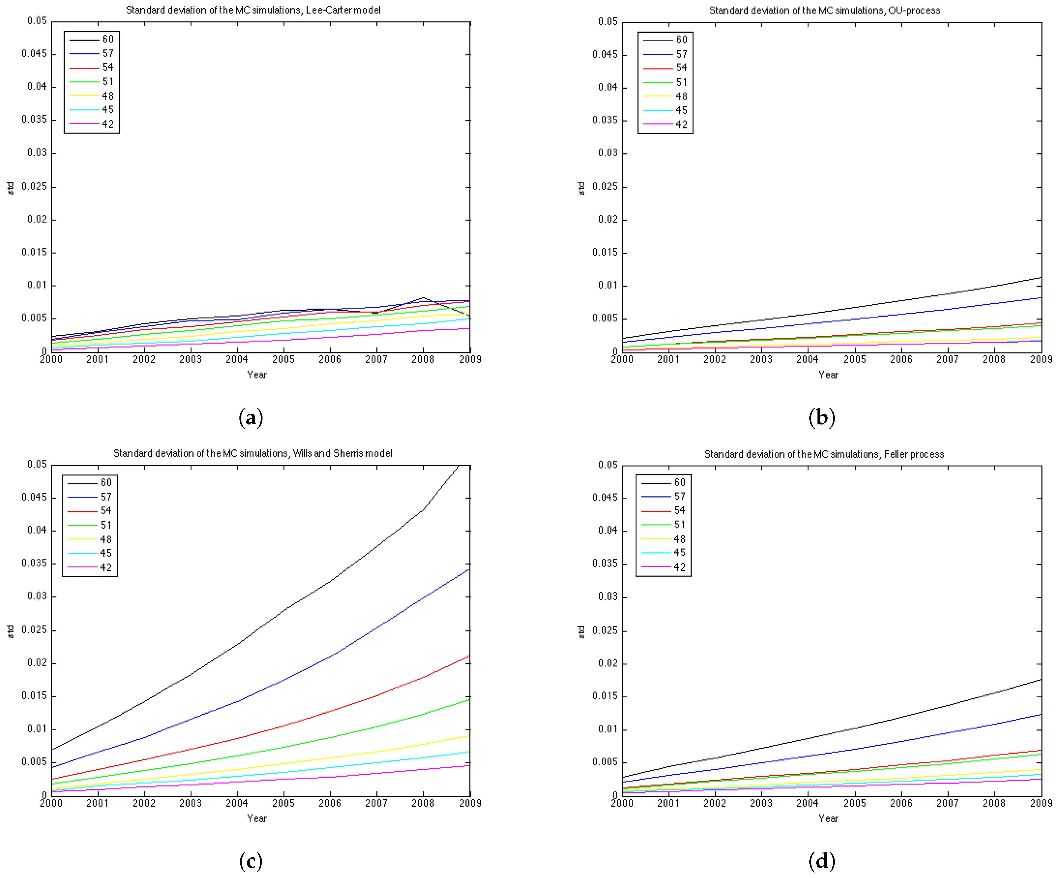
For the Lee Carter model, the variance of the logarithm of the mortality rate at time t for each age x, is , where is the variance of the random walk process , in our case equal to 0.9154, and t is the time passed.
To understand better the variance of the distribution of mortality rates at each point in time we show the graphs of the standard deviation in
Figure 8. The variance of each model grows with time, however, for the Wills and Sharris model it grows substantially faster than for other three models. The second fastest growing variance is of the Feller process, then the OU-process and, finally, the Lee-Carter model shows the slowest growth in variance.
Regarding the covariance/correlation across generations and ages, all models employ a different structure. Lee-Carter is a one-factor model, which results in mortality improvements at all ages being perfectly correlated. Wills and Sherris model is designed to capture correlation between the ages. In practice it amplifies the effect of the variance growth over time since in reality the correlation increases with age (see Wills and Sherris [
13]). In fact, in the simulation procedure the Wiener process is multiplied by the instantaneous correlation matrix
D which describes the correlation structure between ages. The OU and the Feller processes in the current study do not take into account the correlation between generations. However, they can also be extended to the case of multiple generations. In [
27] it is described how the OU process can be extended to the case of two generations, whose changes in mortality intensities are correlated with an instantaneous correlation coefficient.
7.3. Discussion on the Number of Parameters
The number of estimated parameters is different for each procedure. The Wills and Sherris model estimates only 3 parameters for the whole dataset plus eigenvectors to approximate the correlation matrix (in our case we take 30 eigenvectors), while both the OU and the Feller processes fit 2 parameters for each generation. To calibrate the Lee-Carter model, we have to estimate parameters. To predict mortality for each generation in the dataset for which the size of the estimation part would be not be less that 10 years, we have to estimate the OU and the Feller processes for 19 generations resulting in 38 parameters each, for the Wills and Sherris model we have used 3 + 30 = 33 parameters.
7.4. Prediction Intervals
The results of the experiments based on prediction intervals are presented in the
Figure 9 and
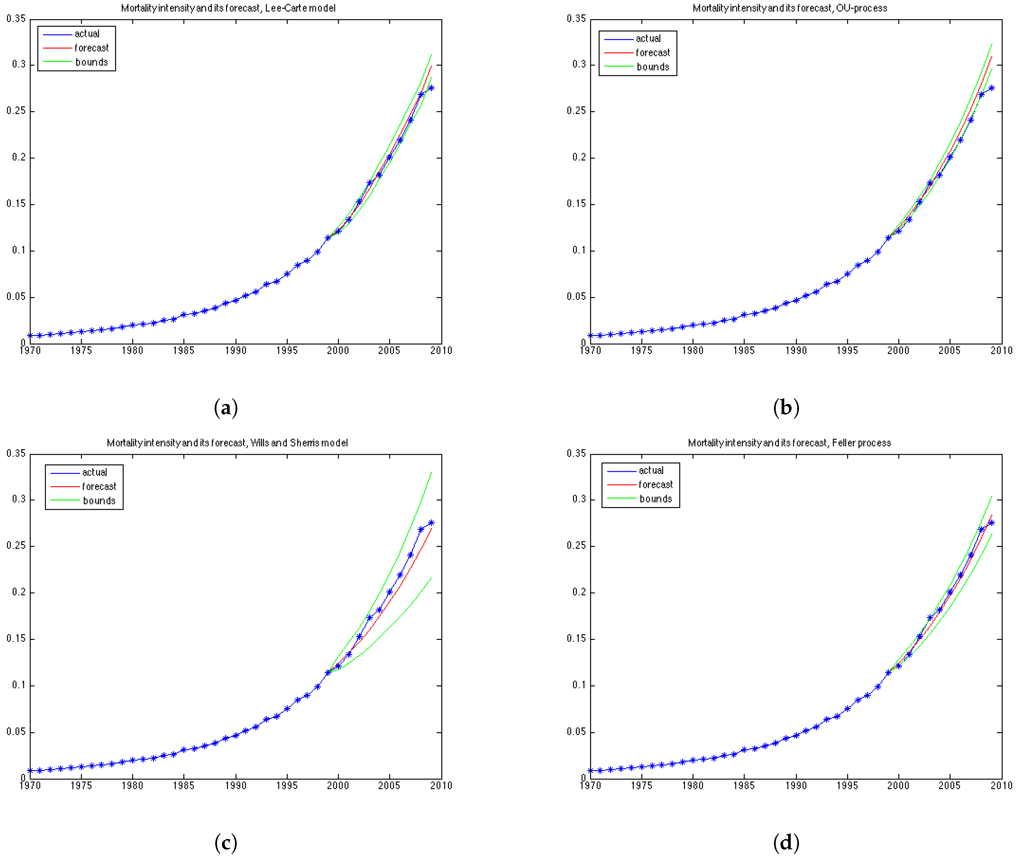
Table 7.
Figure 9 illustrates the 90% prediction intervals built for each model with 15000 MC simulations for generation aged 57 in 1970. We can see that the width of the intervals is different for each model—it is the smallest for the OU-process; medium for the Lee-Carter model and the Feller process, and it is the widest for the Wills and Sherris model, especially for the older ages.
According to
Table 7, the Wills and Sherris model shows the best results in terms of the percentage of the actual future mortality which appear within the confidence bounds—for 15 out of 19 generations the percentage reaches
. The Lee-Carter model and the Feller process results are comparably good, while the OU process shows the worst result with the average percentage of the actual mortality within the prediction intervals being
(
Table 7).
Note, that although the variances of the Lee Carter model is smaller than the ones produced by the OU-process and the Feller process, the first model shows better results.
8. Robustness of Simulation Results
Here we evaluate the performance of the approach described above on the 4 datasets. They are:
UK Females
UK Males
Australian Females
Australian Males
The experiments in this section are made using the same time and the age periods—1970–2009 and 50–99. The generations aged 42–60 in the year 1970 are chosen in the same manner as in
Section 6 and
Section 7.
The results of the estimation are presented in
Table 8 and
Table 9. More detailed results of the estimation for the 4 datasets are included in the
Appendix as tables and plots of the errors for each of the 19 generations. According to the
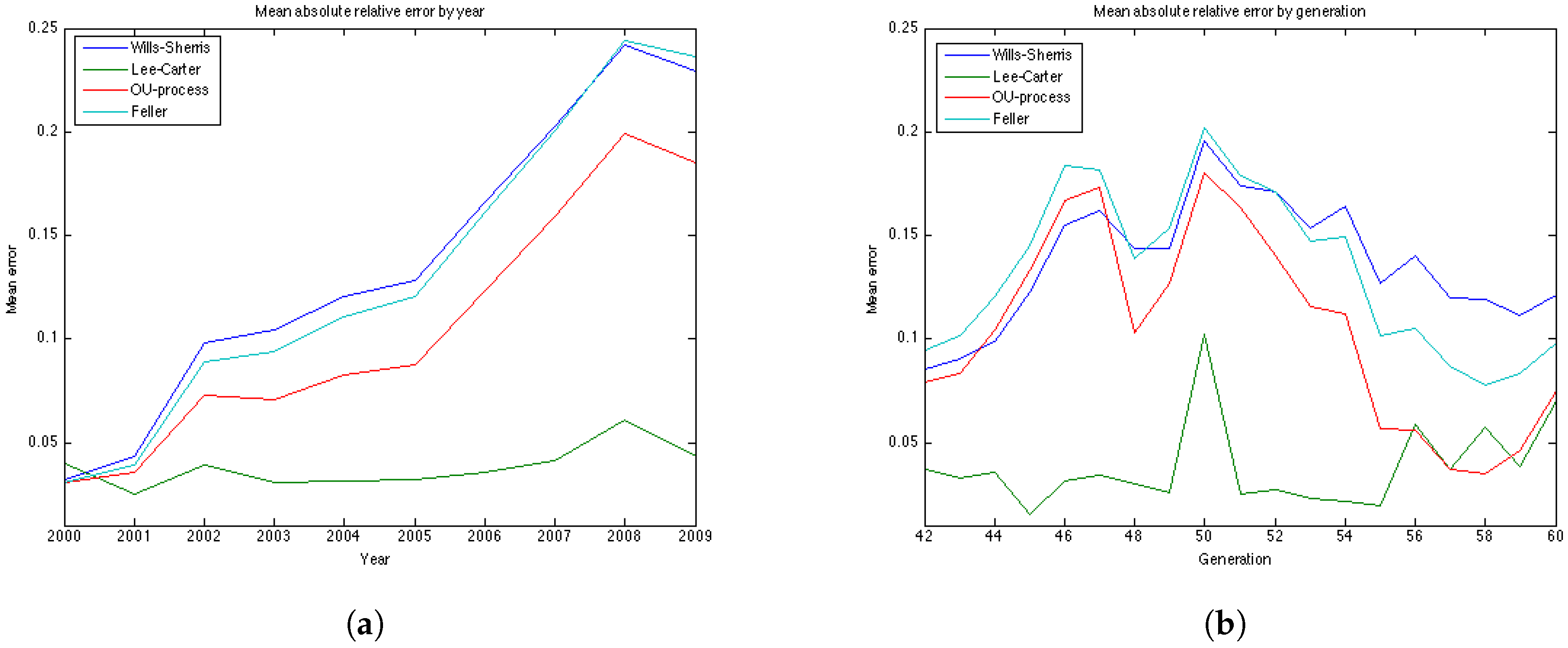
Table 8 and
Table 9, the results for the UK males data with regard to accuracy are the same as for the UK females—the OU and the Feller processes produce the smallest error, while the Lee-Carter and the Wills and Sherris models show the largest error. However, the mean of the absolute error for the Lee-Carter model in this case is 3 times larger in comparison to the error of the UK females estimation. This model also shows very bad result according to precision (with the percentage of the actual mortality within prediction interval being only
).
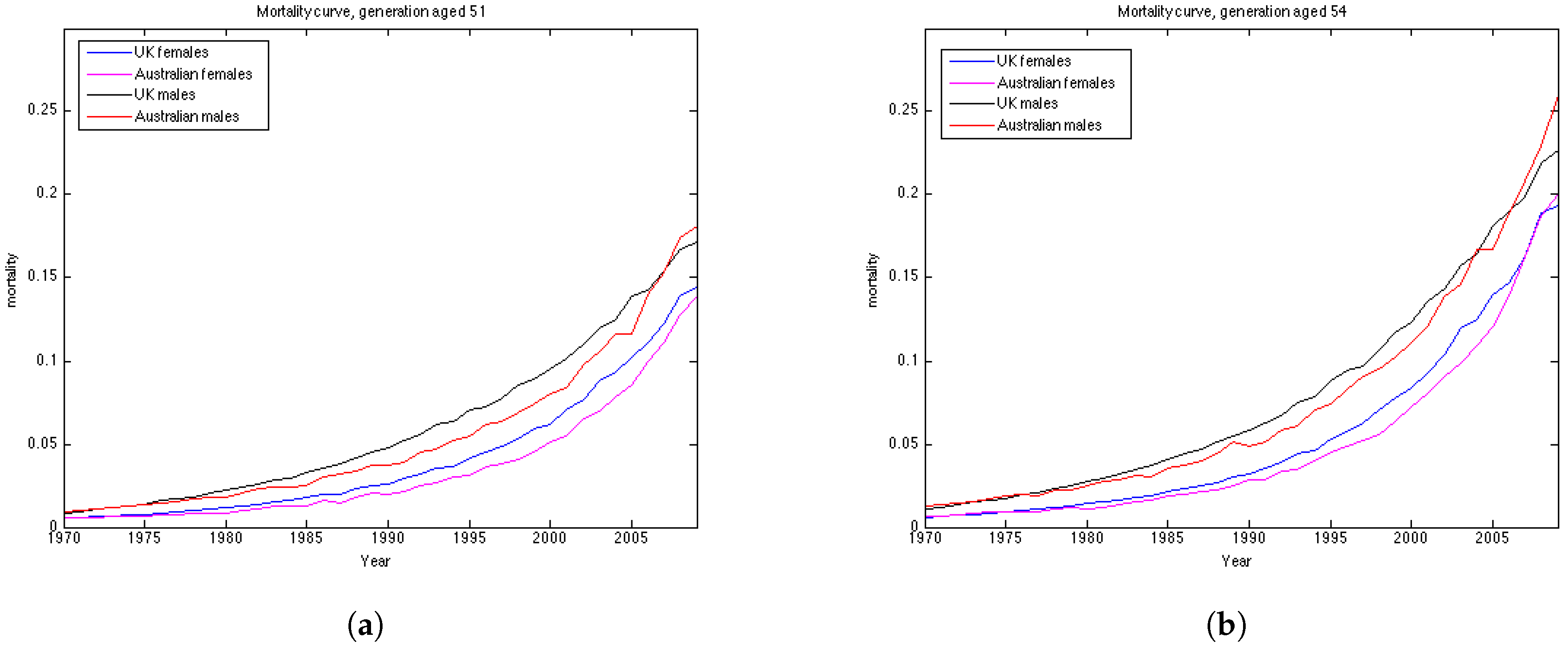
Australian females data is the only dataset which shows good results using the Lee Carter model, both according to precision and accuracy. The OU and the Feller processes, on the contrary, produce large errors for this dataset, especially for the generations aged 45–55. This may be explained by the fact that mortality in Australia is lower for people in their 40s and 50s in comparison to their UK counterparts, and, as a consequence, mortality intensities are larger for older ages. This can be seen from the plots of mortality curves for generations aged 51 and 54 in the year 1970 (
Figure 10). More prominent convex form of the mortality curves for Australian population makes the error (which is calculated for the last 10 years of the observations) larger as the prediction of mortality underestimates the actual mortality intensity. We would suggest that the inclusion of the correlation coefficient for the OU and the Feller processes to describe the dependence between the generations could improve the calibration results for these procedures by taking into account the fact that if mortality of the generations aged 45–55 is rather low, it would imply an increase in the mortality intensity for the older ages.
It is worth noting that for all datasets the errors produced by the Wills and Sherris model, the OU process and the Feller process exhibit similar patterns (
Figure 7b,
Figure 11b,
Figure 12b and
Figure 13b), while the errors produced by the Lee-Carter model have a different pattern. This may be explained by the fact that the first three procedures model the advances (changes) in mortality intensity for a cohort, while the Lee-Carter models the central mortality rate itself.
On the whole, we can say that the results are data dependent. However, from the estimation results on the four datasets, we can conclude that the Wills and Sherris model performs best in terms of precision, but it is one of the worst in terms of accuracy. The Lee Carter model shows better fit to the Australian population dataset rather that to the British one, both for males and females. The OU process and the Feller process provide rather good results in terms of accuracy, while they have often get low ranks in terms of precision.
9. Conclusions
In this study we have calibrated 4 mortality models to the UK and Australian populations and have quantitatively compared their accuracy and precision in forecasting mortality rates. To evaluate this we have used two measures – first, we looked at the relative errors between the forecasted and the observed mortality rates and second, we investigated the percentage of the observed mortality rates which fell within the projected prediction intervals. Our experiments compare one discrete-time model, proposed by Lee and Carter, and three continuous-time models—the Wills and Sherris model, the Ornstein-Uhlenbeck process and the Feller process. The first two models estimate the whole surface of mortality across ages and years simultaneously, while the latter two model each generation separately. One major advantage of the OU and the Feller processes is that they belong to the affine class of mortality models and so allow closed-form expressions for survival probabilities, which is useful for pricing many financial securities. On the other hand, the Wills and Sherris model allows the dependencies between generations to be captured, which may be useful for life offices who have portfolios written on multiple cohorts.
The choice of the model may depend on the goal and the data available. As a result of our experiments with the UK female, the Wills and Sherris model performs best in terms of the prediction interval, followed by the Lee-Carter model. In terms of the mean absolute error, the OU and the Feller processes are better. Thus, for the UK data models which capture the whole mortality surface are more precise, meaning that their forecast prediction intervals are more likely to include the observed mortality rates. Models for a single generation, on the other hand, tend to be more accurate, meaning that their mean absolute errors between the forecast and observed mortality are smaller. For the UK male data the results are rather similar—the main difference here is that the LC model in this case provides much worst result both in terms of precision and accuracy.
However, the results are different for the Australian dataset. In this case, the Lee-Carter model and the OU process are the best in terms of accuracy, both for males and females. The Wills and Sherris model shows good result with respect to the precision measure for Australia as well, followed by the LC for the females and the Feller process for the males.
Based on our experiments, different models appear to be preferred for specific generations and years. We believe that our analysis and the results discussed in this paper are useful for the insurance industry. In particular, we provide potentially useful insights into different mortality modelling frameworks and allow practitioners to chose a model that suits their specific needs.


