Beyond Volatility: A Leakage-Safe Residual-Stress Signal for Drawdown Risk Monitoring

Abstract

Monitoring equity drawdown risk requires real-time indicators that can be implemented without look-ahead bias and that may add information beyond standard volatility measures. This study develops a leakage-safe residual-stress indicator from cross-sectional PCA reconstruction errors in U.S. sector excess returns. Using daily adjusted prices for SPY and 11 U.S. sector ETFs, sector excess returns are computed relative to SPY, the common component is estimated with principal component analysis (PCA), and residual stress is defined as the cross-sectional root-mean-square magnitude of out-of-sample reconstruction residuals. The PCA mapping is estimated using information available only through $t-1$, the stress score is computed at t, and high-stress regimes are defined using rolling train-only quantile thresholds shifted forward by one trading day. The results show that realized volatility remains the stronger standalone benchmark in overall early-warning classification performance. Residual stress is therefore not proposed as a replacement for volatility. Instead, it is most useful as a complementary indicator of cross-sectional market dislocation. In the baseline sample, residual-stress spikes cluster around several drawdown-onset episodes, and conditional regime analysis shows that when volatility is low, high residual stress is associated with a higher probability of a drawdown onset within the next $H=21$ trading days than the low-stress/low-volatility regime. Event-overlap and lead-time diagnostics suggest that residual stress can identify some onset episodes not captured by a simple volatility-threshold rule, although its main incremental value lies in conditional risk stratification rather than systematically earlier triggering. The contribution of the paper is to develop a leakage-safe and interpretable residual-stress diagnostic for conditional drawdown-risk monitoring. The evidence supports a balanced interpretation: residual stress adds state-dependent information beyond standard volatility measures, especially in otherwise low-volatility states, but it does not dominate realized volatility as a standalone predictor.

1. Introduction

Large equity drawdowns are economically costly and difficult to anticipate using stable linear predictors alone. In practice, the objective is not precise return forecasting, but risk-state detection: identifying periods in which downside risk is elevated so that investors and risk managers can adjust exposure, hedging intensity, and monitoring decisions in real time. This paper studies whether a leakage-safe measure of cross-sectional residual stress contains complementary information about drawdown risk beyond standard volatility- and correlation-based signals.

The starting point is that sector returns often share a low-dimensional common structure driven by broad market and macroeconomic forces (Jolliffe 2002; Ross 1976; Yang et al. 2017). During periods of market stress, however, sector-level repricing may become less well described by that dominant common component. Prior studies on idiosyncratic volatility, herding behavior, and cross-sectional return dispersion suggest that residual or sector-specific movements can contain information about changing market conditions (Campbell et al. 2001; Chang et al. 2000; Christie and Huang 1995). We interpret this residual fragmentation as a potentially informative dimension of market stress. To measure it, we apply principal component analysis (PCA) (Jolliffe 2002) to sector excess returns (sector minus SPY), extract a low-dimensional common component, and define residual stress as the cross-sectional root-mean-square magnitude of out-of-sample PCA reconstruction residuals. Intuitively, the signal rises when sector movements become increasingly misaligned with the dominant low-dimensional market structure.

The central question is whether this residual-stress signal captures information not already summarized by conventional market-stress measures. This distinction matters because realized volatility measures the time-series amplitude of aggregate market fluctuations, while rolling pairwise correlation measures average sector comovement. Realized volatility is used as the main benchmark because volatility-managed and risk-controlled exposures are widely used in portfolio risk management (Barroso and Santa-Clara 2015; Moreira and Muir 2017). Rolling average pairwise correlation is also included as a benchmark because crisis-period comovement and correlation increases are central issues in the contagion and interdependence literature (Dungey et al. 2005; Forbes and Rigobon 2002). Both volatility and correlation are important benchmarks, but they may not fully capture cross-sectional dislocation after the dominant common component has been removed. Residual stress is designed to measure this remaining residual fragmentation. The contribution of the paper is therefore not to propose residual stress as a replacement for realized volatility or correlation, but to test whether it provides complementary, state-dependent, and event-level information for drawdown-risk monitoring under a leakage-safe design.

A further contribution is implementation discipline. At each date t, the PCA mapping, including centering and loadings, is estimated using information available only through $t-1$, and the residual-stress score is then computed out-of-sample for date t. High-stress regimes are identified using a rolling train-only quantile threshold constructed only from historical stress scores and shifted forward by one trading day, so that the regime label used for monitoring at t depends only on information available through $t-1$. This timing discipline is designed to avoid look-ahead bias and to permit a clean evaluation of real-time warning performance.

Empirically, the paper evaluates the signal using daily U.S. sector ETF data and compares results across three sample windows: 2015–2019, 2020–2025, and 2015–2025. The 2015–2019 period provides a pre-pandemic benchmark, while the 2020–2025 period captures a modern stress-heavy sample that includes the COVID-19 market shock, the subsequent inflationary period, monetary-policy tightening, and sector-specific repricing episodes (Acharya and Steffen 2020; Pandey 2025). The full 2015–2025 period evaluates whether the results remain stable across both calmer and more turbulent regimes. This subperiod design helps separate evidence that is specific to the unusual post-2020 environment from evidence that is more stable across market conditions.

Drawdown-warning performance is evaluated using drawdown-onset events, event-study visualizations, and early-warning classification metrics including ROC-AUC, PR-AUC, and horizon-H precision and recall. ROC-AUC is included because it summarizes the ranking ability of a continuous warning score across thresholds, while PR-AUC is especially relevant when positive events are rare (Davis and Goadrich 2006; Hanley and McNeil 1982). Because volatility-based indicators are natural benchmarks for market stress and risk timing (Barroso and Santa-Clara 2015; Moreira and Muir 2017), all evaluations compare residual stress against realized volatility under the same leakage-safe timing protocol. The paper also reports rolling pairwise sector correlation as a main benchmark because crisis-period comovement may overlap with volatility-based signals (Dungey et al. 2005; Forbes and Rigobon 2002). Additional diagnostics examine event overlap, lead time, conditional risk regimes, and whether residual stress identifies onset episodes not captured by simple volatility- or correlation-threshold rules.

The analysis also examines robustness to key modeling choices. The baseline specification uses a fixed number of principal components and an expanding PCA window. To assess whether the findings depend on these choices, the paper reports robustness checks using rolling 252-day and 504-day PCA windows, data-driven factor-number selection using the information criteria of (Bai and Ng 2002), and an idiosyncratic-volatility-scaled version of residual stress. These tests address whether the residual-stress signal is stable when the common-factor structure changes across regimes and when sector-specific heteroskedasticity is explicitly controlled.

This study differs from related work on volatility forecasting, drawdown-risk measurement, and machine learning early-warning systems in both object and mechanism (Ciciretti et al. 2025; Davis and Goadrich 2006; Geboers et al. 2023; Liu 2026; Moreira and Muir 2017). Rather than forecasting volatility itself or benchmarking flexible classifiers on broad cross-asset predictors, it asks whether cross-sectional residual dislocation across sector ETFs contains useful information for equity drawdown-risk monitoring after the dominant common market structure has been removed. Therefore, its contribution lies in residual market-structure diagnostics and leakage-safe evaluation, rather than in volatility prediction or generic predictive-model comparison.

The main finding is deliberately balanced. Realized volatility remains the stronger standalone benchmark in the baseline classification results. Residual stress is therefore best interpreted as a complementary diagnostic rather than a replacement for volatility. Its main value lies in conditional drawdown-risk stratification, especially in otherwise low-volatility states where elevated residual fragmentation may reveal market dislocation not fully summarized by aggregate volatility or average correlation. The analysis links this evidence to a feasible real-time monitoring framework while distinguishing monitoring value from standalone trading profitability.

The remainder of the paper is organized as follows. Section 2 reviews related work. Section 3 describes the data, leakage-safe signal construction, benchmark signals, and drawdown-onset definition. Section 4 reports early-warning performance, conditional-risk evidence, robustness checks, and practical applications. Section 5 discusses interpretation and limitations. Section 6 concludes.

2. Literature Review

This paper relates to four strands of research: (i) low-dimensional factor structure and statistical decompositions of asset returns, (ii) cross-sectional dispersion, correlation, and market-stress measurement, (iii) drawdown-risk monitoring and early-warning evaluation, and (iv) risk-managed overlays and implementable trading rules.

2.1. Low-Dimensional Return Structure and PCA-Based Decompositions

A large amount of literature models asset returns using a small number of common factors. Multi-factor asset-pricing frameworks provide an economic motivation for decomposing returns into common and idiosyncratic components, while statistical factor models and dimensionality-reduction methods estimate latent low-rank structure directly from return panels when the number or identity of the underlying factors is uncertain (Koutoulas and Kryzanowski 1994). Within this literature, principal component analysis (PCA) is a standard tool for extracting dominant comovement and isolating an orthogonal residual component (Jolliffe 2002; Yang et al. 2017). PCA has also been used in empirical studies of stock-market behavior across major financial exchanges, illustrating its usefulness for summarizing multivariate market comovement (Quiroga-Juárez and Villalobos-Escobedo 2025).

In this paper, PCA is used as a parsimonious statistical filter rather than as a structural asset-pricing model. Applied to sector excess returns, defined as sector returns minus SPY returns, PCA removes the dominant common component and produces a residual panel that captures cross-sectional movements not explained by the leading low-dimensional market structure (Arai et al. 2013; Yang et al. 2017). This residual component provides the basis for the paper’s stress measure. Because the estimated factor structure may change across regimes, the empirical analysis also examines whether the results are robust to alternative PCA windows and to data-driven selection of the number of retained factors.

The choice of the number of common components is important in approximate factor models. A fixed value of K is transparent and easy to interpret, but it may be too restrictive if the strength or dimension of the common factor structure changes across market regimes. For this reason, the robustness analysis compares the baseline fixed-K specification with factor-number selection using the information criteria of (Bai and Ng 2002). This comparison helps assess whether the residual-stress results are driven by an arbitrary choice of retained principal components.

2.2. Cross-Sectional Dispersion, Correlation, and Market Stress

Beyond aggregate market volatility, cross-sectional return dispersion and residual variation can contain information about market conditions. Elevated dispersion may reflect disagreement, dislocation, sector rotation, or fragmentation that is not fully summarized by broad market moves (Campbell et al. 2001; Chang et al. 2000; Christie and Huang 1995). Related ideas also appear in research on herding, disagreement, and uncertainty measures constructed from return panels and other financial data.

However, raw cross-sectional dispersion is not the same as residual stress. Raw dispersion can increase because of broad market movements, sector-level volatility differences, or changing correlations. Residual stress is more targeted because it is computed after removing the dominant common sector component through PCA. It therefore measures the part of sector movement that remains unexplained by the estimated common structure. This distinction is important for the paper’s contribution: the proposed signal is not simply another volatility or raw dispersion measure, but an interpretable diagnostic of residual market fragmentation.

Average pairwise correlation provides another important benchmark. During market stress, correlations often rise mechanically with aggregate volatility, making it difficult to distinguish genuine incremental information from general market comovement. This issue is closely related to the contagion and interdependence literature, which emphasizes that higher measured correlations during crises may partly reflect increased volatility rather than a separate transmission mechanism. For this reason, this paper treats rolling pairwise sector correlation as a main benchmark rather than only an auxiliary robustness check. The empirical question is whether residual stress contains conditional information beyond both realized volatility and average sector correlation.

This distinction motivates the comparison with rolling pairwise correlation. Prior work shows that measured cross-market correlations can increase during turbulent periods partly because of higher volatility, complicating the interpretation of crisis-period comovement (Forbes and Rigobon 2002). Related contagion studies also emphasize that empirical tests must distinguish genuine transmission effects from common shock and interdependence channels (Dungey et al. 2005). In this paper, rolling pairwise sector correlation is therefore treated as a main benchmark rather than an auxiliary control, while residual stress is evaluated as a distinct measure of cross-sectional fragmentation after removal of the estimated common PCA component.

2.3. Drawdown Risk and Early-Warning Evaluation

Predicting drawdowns is difficult because downside events are infrequent, nonlinear, and often regime-dependent (Ciciretti et al. 2025; Geboers et al. 2023). A common response is to frame the problem as one of risk-state detection or early warning, where the goal is not precise return forecasting but timely identification of elevated downside risk. In this setting, event-based definitions and classification-oriented metrics are often more informative than average return predictability alone.

This paper therefore evaluates residual stress using drawdown-onset labels and early-warning classification metrics, including ROC-AUC, PR-AUC, and horizon-H precision and recall. ROC-AUC summarizes the ranking ability of a continuous score across thresholds, while PR-AUC is especially useful when positive events are rare (Davis and Goadrich 2006; Hanley and McNeil 1982). Because drawdown onsets are infrequent, the analysis also reports event-level diagnostics, conditional regime comparisons, and moving-block bootstrap evidence to assess the stability of the results under serial dependence and small-event samples.

2.4. Risk-Managed Overlays and Implementable Trading Rules

In portfolio applications, early-warning or regime signals are often mapped into overlays that reduce exposure during stress periods, trading off protection against turnover, tracking error, and transaction costs (Ciciretti et al. 2025). Related literature studies volatility-managed and risk-controlled exposures as implementable tools for drawdown mitigation (Barroso and Santa-Clara 2015; Moreira and Muir 2017). These applications are relevant because a risk-monitoring signal is more useful if it can be translated into an implementable decision rule.

Consistent with this perspective, this paper reports illustrative transaction-cost-aware applications, including a stress-managed SPY overlay and a residual-ranked sector long–short portfolio. These exercises are not treated as the primary evidence for the signal’s value. Instead, they illustrate how the monitoring signal behaves when mapped into feasible portfolio rules under lagged timing and explicit transaction costs. The analysis also considers higher transaction-cost assumptions because trading frictions may increase during stressed markets.

2.5. Positioning of This Work

This paper sits at the intersection of several related studies, but its objective differs from each of them in a specific way. Unlike volatility-forecasting studies, it does not seek to improve forecasts of market variance; instead, it asks whether cross-sectional residual fragmentation contains information about future drawdown onsets beyond realized volatility. Unlike PCA and statistical factor-model studies, it does not treat latent factors as the main empirical object. PCA is used here as a filtering step to remove the dominant common sector structure, after which the residual component is interpreted as a measure of cross-sectional dislocation. Relative to the broader literature on cross-sectional dispersion, disagreement, herding, and correlation, the proposed measure is more targeted because it is constructed from residual rather than raw sector excess returns. Unlike general machine learning early-warning studies, the paper emphasizes an interpretable signal, onset-based evaluation, and an implementable train-only timing protocol rather than classifier complexity. Machine-learning forecasting models, including LSTM-based approaches, have also been applied to portfolio optimization and financial prediction tasks (Li and Liu 2023).

The contribution is therefore not a new forecasting architecture or a claim of predictive dominance over realized volatility. Instead, the paper provides evidence on whether residual cross-sectional stress can improve conditional drawdown-risk monitoring within a leakage-safe framework. This positioning is important because the empirical results show that realized volatility remains the stronger standalone benchmark, while residual stress is most useful as a complementary diagnostic for conditional risk stratification.

3. Methodology

3.1. Data, Return Construction, and Reproducibility

The empirical design uses sector-based U.S. equity panels to evaluate whether the residual-stress signal is stable across market environments. The main investable sample consists of the S&P 500 ETF (SPY) and 11 sector ETFs: XLC, XLY, XLP, XLE, XLF, XLV, XLI, XLK, XLB, XLU, and XLRE. To address the possibility that the 2020–2025 period is unusual because of pandemic, inflation, monetary-policy, and sector-specific shocks, the analysis compares three sample windows: 2015–2019, 2020–2025, and 2015–2025. The 2015–2019 window provides a pre-pandemic benchmark, the 2020–2025 window corresponds to the contemporary stress-heavy period, and the full 2015–2025 window evaluates stability across both calmer and more turbulent regimes.

The paper also reports a longer-history proxy-sector panel spanning 1 January 1999 to 31 December 2025. This proxy sample is used as an additional robustness check to assess whether the same conditional and event-level patterns remain stable across a larger number of drawdown episodes. The proxy analysis is not treated as the main investable ETF benchmark; rather, it provides broader historical evidence about the stability of the residual-stress mechanism.

Daily adjusted close prices are downloaded from Yahoo Finance. Adjusted prices are used to account for dividends and stock splits. After download, all series are aligned to a common trading calendar, and any date with missing observations in any ETF is removed to ensure a balanced panel. The same alignment and reproducibility rules are applied within each sample window so that signal construction and evaluation remain comparable across subperiods.

Let $P_{i,t}$ denote the adjusted close price of sector ETF i on day t, and let $P_{m,t}$ denote the adjusted close price of SPY. Simple daily returns are computed as

$$r_{i,t}={\displaystyle \frac{P_{i,t}}{P_{i,t-1}}}-1,r_{m,t}={\displaystyle \frac{P_{m,t}}{P_{m,t-1}}}-1.$$

(1)

To isolate sector-specific movements beyond the broad market component, we define sector excess returns as

$$x_{i,t}=r_{i,t}-r_{m,t}.$$

(2)

Stacking these across the $N=11$ sectors yields the cross-sectional excess-return vector

$${\mathbf{x}}_t={(x_{1,t},\dots ,x_{N,t})}^{\top }\in {\mathbb{R}}^N,$$

(3)

and collecting observations over $t=1,\dots ,T$ gives the return panel

$$\mathbf{X}=\left[\begin{array}{c}{\mathbf{x}}_1^{\top }\\ ⋮\\ {\mathbf{x}}_T^{\top }\end{array}\right]\in {\mathbb{R}}^{T\times N}.$$

(4)

All data used in this study are publicly available. Daily adjusted close prices are retrieved from Yahoo Finance via quantmod. The empirical design, sample-window definitions, parameter choices, and leakage-safe timing protocol are described in detail to support reproducibility. The study does not redistribute raw price data; instead, the data can be retrieved directly from the public source. All signal construction, thresholding, benchmarking, and portfolio-evaluation steps are implemented using the train-only timing conventions described in the following subsections.

3.2. Leakage-Safe PCA Residual-Stress Construction

The paper measures cross-sectional market stress using the residual component of sector excess returns after removing a low-dimensional common structure. Let ${\mu }_{t-1}\in {\mathbb{R}}^N$ denote the training-sample mean of sector excess returns, estimated using only information available through $t-1$. In the baseline specification, we use an expanding-window PCA with an initial burn-in window of $W_{\mathrm{PCA}}=252$ trading days. The centered excess-return vector at date t is

$${\tilde{x}}_t=x_t-{\mu }_{t-1}.$$

(5)

In the baseline specification, the common component is restricted to the first two principal components ($K=2$), corresponding to PC1 and PC2. This fixed-K design is transparent and easy to interpret. However, because the dimension of the common-factor structure may change across market regimes, the robustness analysis also allows K to be selected within each training window using the information criteria of (Bai and Ng 2002).

Out-of-sample PCA projection. Let $L_{t-1}=[{\mathcal{l}}_{1,t-1},\dots ,{\mathcal{l}}_{K,t-1}]\in {\mathbb{R}}^{N\times K}$ denote the orthonormal loading matrix obtained by applying PCA to the centered training sample through $t-1$, so that

$$L_{t-1}^{\top }{L}_{t-1}=I_K.$$

(6)

The corresponding out-of-sample factor score for day t is

$$f_t=L_{t-1}^{\top }{\tilde{x}}_t\in {\mathbb{R}}^K.$$

(7)

The rank-K common-component reconstruction is then

$${\widehat{x}}_t=L_{t-1}{f}_t=L_{t-1}{L}_{t-1}^{\top }{\tilde{x}}_t.$$

(8)

Residual vector and stress score. The residual vector is defined as the reconstruction error

$$e_t={\tilde{x}}_t-{\widehat{x}}_t=\left(I_N-L_{t-1}{L}_{t-1}^{\top }\right){\tilde{x}}_t\in {\mathbb{R}}^N.$$

(9)

By construction, $e_t$ is orthogonal to the estimated factor space:

$$L_{t-1}^{\top }{e}_t=0.$$

(10)

This study summarizes the cross-sectional magnitude of these residuals using the root-mean-square (RMS) residual-stress score

$${\mathrm{Stress}}_t=\sqrt{{\displaystyle \frac{1}{N}}\sum _{i=1}^N{e}_{i,t}^2}.$$

(11)

Intuitively, ${\mathrm{Stress}}_t$ rises when sector movements are less well captured by the dominant low-rank common structure.

Throughout, the PCA mapping and the stress score at date t are constructed using only information available through $t-1$. This timing discipline ensures that ${\mathrm{Stress}}_t$ is implementable in real time and free of look-ahead bias. PCA provides the standard rank-K least-squares approximation to the centered training panel, so the residual vector can be interpreted as the component of sector excess returns not explained by the leading low-dimensional common structure.

3.3. Alternative PCA Windows and Factor-Number Selection

The baseline specification uses an expanding-window PCA estimator with an initial burn-in window of $W_{\mathrm{PCA}}=252$ trading days. Expanding-window estimation preserves all historical information, but it may adapt slowly after structural breaks because older regimes remain in the estimation sample. To assess this issue, the robustness analysis also estimates PCA loadings using rolling windows of 252 and 504 trading days. The 252-day window allows the common-factor structure to adapt quickly to recent market conditions, while the 504-day window provides a smoother two-year estimate. In all cases, the PCA loadings used at date t are estimated only from observations available through $t-1$.

The baseline specification fixes the number of retained components at $K=2$. To examine whether the results depend on this choice, the robustness analysis also selects K within each training window using the information criteria of (Bai and Ng 2002). The selected-K residual-stress score is then computed using the same out-of-sample projection and leakage-safe timing protocol as the baseline specification. Comparing fixed-K and selected-K results helps determine whether the residual-stress evidence is driven by an arbitrary factor-number choice.

3.4. Idiosyncratic-Volatility-Scaled Residual Stress

The baseline residual-stress score defined in Equation (11) is the cross-sectional RMS magnitude of PCA residuals. A potential concern is that sectors with naturally larger idiosyncratic volatility may contribute disproportionately to the unscaled index. To address this concern, the robustness analysis also computes an idiosyncratic-volatility-scaled version of residual stress.

Let ${\widehat{\sigma }}_{i,t-1}^{\mathrm{idio}}$ denote the rolling standard deviation of sector i’s PCA residuals, estimated using only residuals observed through $t-1$. The standardized residual is

$$z_{i,t}={\displaystyle \frac{e_{i,t}}{{\widehat{\sigma }}_{i,t-1}^{\mathrm{idio}}}}.$$

(12)

The scaled residual-stress score is then

$${\mathrm{Stress}}_t^{\mathrm{scaled}}=\sqrt{{\displaystyle \frac{1}{N}}\sum _{i=1}^N{z}_{i,t}^2}.$$

(13)

This specification measures abnormal residual dispersion relative to each sector’s own historical residual volatility and reduces the possibility that the stress index is mechanically dominated by persistently high-volatility sectors. The rolling idiosyncratic-volatility estimate is shifted forward by one trading day so that the scaled score remains implementable in real time.

3.5. Train-Only Regime Construction and Implementable Timing

To maintain a leakage-safe design, any quantity used for labeling, benchmarking, or trading at date t is constructed using information available no later than $t-1$.

Train-only stress threshold. Using a lookback window of length $W_{\mathrm{thr}}$ and quantile level q, we compute the rolling train-only threshold

$$Q_{t-1}^{\left(q\right)}={\mathrm{Quantile}}_q\left({\mathrm{Stress}}_{t-W_{\mathrm{thr}}},\dots ,{\mathrm{Stress}}_{t-1}\right),$$

(14)

and define the stress-regime indicator as

$${\mathbb{I}}_t^{\mathrm{stress}}=\mathbb{1}\left\{{\mathrm{Stress}}_t>Q_{t-1}^{\left(q\right)}\right\}.$$

(15)

In implementation, the rolling quantile in Equation (14) is evaluated with a right-aligned window and shifted forward by one trading day, so that the threshold applied at date t depends only on historical stress values observed through $t-1$.

Lagged, implementable signals. Any strategy or overlay that depends on the stress regime uses the lagged label ${\mathbb{I}}_{t-1}^{\mathrm{stress}}$ to set exposure for day t. Likewise, sector-ranking signals for the long–short application are formed from the lagged residual vector $e_{t-1}$, portfolio weights are set at the close of $t-1$, and realized portfolio returns are computed using contemporaneous excess returns ${\mathbf{x}}_t$. This convention ensures that both regime identification and portfolio formation are implementable and free of look-ahead bias.

3.6. Drawdown-Onset Events and Horizon-H Early-Warning Labels

SPY drawdown and drawdown-onset events. Let $r_{m,t}$ denote the simple daily return of SPY from Equation (1). Define the cumulative equity curve by

$$E_t=\prod _{\tau \le t}(1+r_{m,\tau }),$$

(16)

and the drawdown series by

$${\mathrm{DD}}_t={\displaystyle \frac{E_t}{{max}_{\tau \le t}{E}_{\tau }}}-1.$$

(17)

Fix a drawdown threshold $\delta <0$ (e.g., $\delta =-10\%$). The drawdown-region indicator is

$${\mathbb{I}}_t^{\mathrm{DD}}=\mathbb{1}\left\{{\mathrm{DD}}_t\le \delta \right\}.$$

(18)

The drawdown-onset event is defined as the first entry into the drawdown region:

$${\mathbb{I}}_t^{\mathrm{onset}}={\mathbb{I}}_t^{\mathrm{DD}}\left(1-{\mathbb{I}}_{t-1}^{\mathrm{DD}}\right).$$

(19)

Thus, ${\mathbb{I}}_t^{\mathrm{onset}}=1$ only on dates when the drawdown crosses below $\delta$ from above, avoiding repeated labels during the same drawdown episode.

Horizon-$\mathit{H}$ early-warning label. For classification-style early warning, we define the binary target

$$y_t^{\left(H\right)}=\mathbb{1}\left\{{\displaystyle \sum _{h=1}^H}{\mathbb{I}}_{t+h}^{\mathrm{onset}}\ge 1\right\},$$

(20)

which equals one if at least one drawdown-onset event occurs within the next H trading days. The corresponding unconditional event rate is

$$\overline{y}={\displaystyle \frac{1}{T}}{\displaystyle \sum _{t=1}^T}{y}_t^{\left(H\right)}.$$

(21)

This study reports sensitivity checks over drawdown thresholds, warning horizons, and regime-threshold definitions while preserving the same leakage-safe timing protocol throughout.

3.7. Benchmark Signals

Main volatility benchmark. Let $r_{m,t}$ denote the simple daily return of SPY from Equation (1). We define realized volatility as the annualized rolling standard deviation of daily SPY returns over a window of length $W_{\mathrm{vol}}$:

$${\mathrm{Vol}}_t=\sqrt{252}·\mathrm{SD}\left(r_{m,t-W_{\mathrm{vol}}+1},\dots ,r_{m,t}\right).$$

(22)

The continuous score ${\mathrm{Vol}}_t$ serves as the main standalone benchmark in ROC/PR evaluation.

Train-only volatility regime.

Analogous to the stress-regime construction, we compute the rolling train-only quantile threshold

$$Q_{t-1,\mathrm{vol}}^{\left(q_{\mathrm{vol}}\right)}={\mathrm{Quantile}}_{q_{\mathrm{vol}}}\left({\mathrm{Vol}}_{t-W_{\mathrm{thr},\mathrm{vol}}},\dots ,{\mathrm{Vol}}_{t-1}\right),$$

(23)

and define the volatility-regime indicator as

$${\mathbb{I}}_t^{\mathrm{vol}}=\mathbb{1}\left\{{\mathrm{Vol}}_t>Q_{t-1,\mathrm{vol}}^{\left(q_{\mathrm{vol}}\right)}\right\}.$$

(24)

As with the stress threshold, the rolling quantile in Equation (23) is right-aligned and shifted forward by one trading day so that the regime label at date t depends only on information available through $t-1$.

Rolling average pairwise sector correlation. Because correlation-based measures are standard indicators of market comovement and may behave differently during stressed markets, rolling average pairwise sector correlation is reported as a main benchmark rather than only as an appendix robustness check. Let ${\rho }_{ij,t-1}$ denote the rolling correlation between sector excess returns i and j, estimated over a historical window ending at $t-1$. The average pairwise correlation score is

$${\mathrm{Corr}}_t={\displaystyle \frac{2}{N(N-1)}}\sum _{1\le i<j\le N}{\rho }_{ij,t-1}.$$

(25)

This score is included as a main benchmark because sector correlations often rise during stress periods and may capture broad market comovement that overlaps with volatility-based signals.

Realized volatility serves as the main standalone benchmark in the baseline comparison, while rolling average pairwise sector correlation serves as the main cross-sectional comovement benchmark. Additional benchmark signals include downside semivolatility, the VIX when available, cross-sectional return dispersion, and a sector breadth measure based on the share of negative excess returns. All benchmark signals are constructed under the same train-only timing discipline as the residual-stress and volatility measures.

3.8. Bootstrap Inference

To assess sampling uncertainty in early-warning metrics and conditional-regime comparisons, the paper uses a moving-block bootstrap that resamples contiguous time-series blocks of daily observations. This procedure preserves short-run serial dependence in signal realizations, early-warning labels, regime indicators, and event-level diagnostics. Bootstrap confidence intervals are reported for selected ROC-AUC, PR-AUC, precision, recall, F1, conditional event-rate differences, event-overlap statistics, and lead-time measures. In addition, bootstrap comparisons are used to assess selected differences in ROC-AUC and PR-AUC across benchmark signals.

Because drawdown onsets are rare, especially in the modern ETF sample, bootstrap evidence is interpreted as a stability diagnostic rather than as definitive proof of statistical dominance. The purpose is to evaluate whether the qualitative conclusions remain stable under resampling of dependent time-series blocks. All bootstrap exercises preserve the same leakage-safe timing protocol as the main analysis.

3.9. Overlay Implementation and Transaction Costs

These portfolio rules are treated as illustrative applications rather than as the primary basis for evaluating the signal. Their purpose is to show how the monitoring signal behaves when mapped into implementable exposure-management rules under lagged timing and explicit transaction costs.

Baseline portfolio return. Let $w_{t-1}$ denote the portfolio weights set at the close of day $t-1$ and held over day t. More generally, let $r_t^{*}$ denote the contemporaneous vector of traded returns, where $r_t^{*}$ corresponds to raw asset returns for the SPY overlay and to sector excess returns for the residual-ranked long–short application. The gross portfolio return is

$$r_{p,t}^{\mathrm{gross}}=w_{t-1}^{\top }{r}_t^{*}.$$

(26)

Overlay rule. Let ${\mathbb{I}}_{t-1}^{\mathrm{ov}}\in \{0,1\}$ denote an implementable overlay trigger known at time $t-1$, such as ${\mathbb{I}}_{t-1}^{\mathrm{stress}}$ or ${\mathbb{I}}_{t-1}^{\mathrm{vol}}$. For overlay intensity $\lambda \in (0,1)$, we scale risky exposure by

$$s_{t-1}=1-\lambda {\mathbb{I}}_{t-1}^{\mathrm{ov}}.$$

(27)

The overlay-adjusted weights are

$${\tilde{w}}_{t-1}=s_{t-1}{w}_{t-1},$$

(28)

so that a “30% overlay” corresponds to $\lambda =0.30$ and reduces risky exposure to $70\%$ of the baseline allocation when the trigger is active. The remaining fraction $1-s_{t-1}$ is allocated to cash with zero return, implying

$${\tilde{r}}_{p,t}^{\mathrm{gross}}={\tilde{w}}_{t-1}^{\top }{r}_t^{*}=s_{t-1}{w}_{t-1}^{\top }{r}_t^{*}.$$

(29)

Transaction costs and net returns. This paper applies proportional transaction costs to portfolio turnover. Let

$${\mathrm{TO}}_t=\sum _i\left|{\tilde{w}}_{i,t}-{\tilde{w}}_{i,t-1}\right|$$

(30)

denote one-way turnover in weights at the rebalance from $t-1$ to t after the overlay is applied. Given a one-way cost rate c, the net return is

$$r_{p,t}^{\mathrm{net}}={\tilde{r}}_{p,t}^{\mathrm{gross}}-c·{\mathrm{TO}}_t.$$

(31)

Unless otherwise stated, the baseline transaction-cost assumption is $c=5$ bps per unit of one-way turnover, and the paper reports performance statistics using the net return series $\left\{r_{p,t}^{\mathrm{net}}\right\}$. Because trading frictions may increase during stressed markets, the robustness analysis also reports higher constant-cost scenarios of 10 bps and 25 bps.

4. Results

4.1. Residual-Stress Dynamics Around Drawdown Onsets

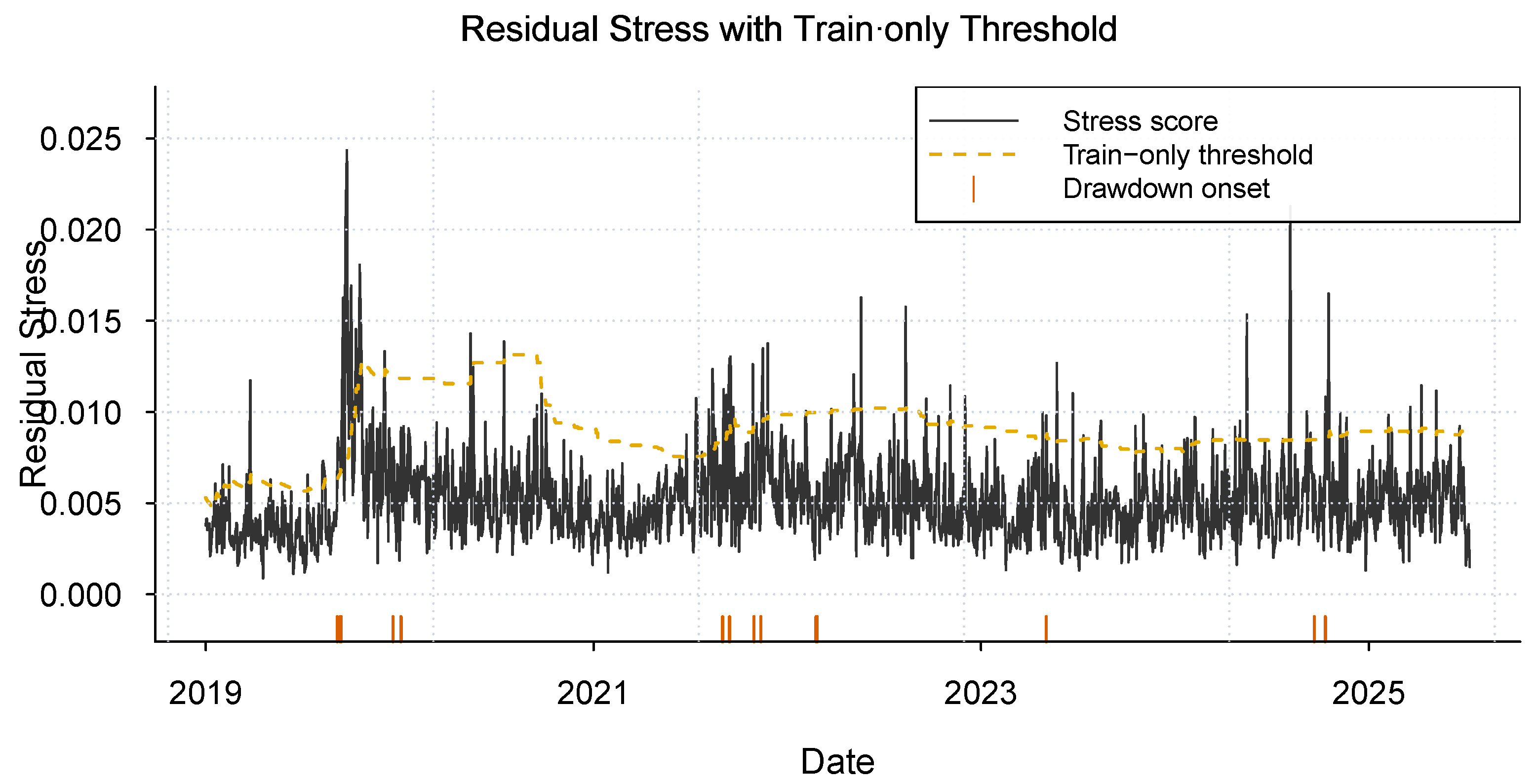
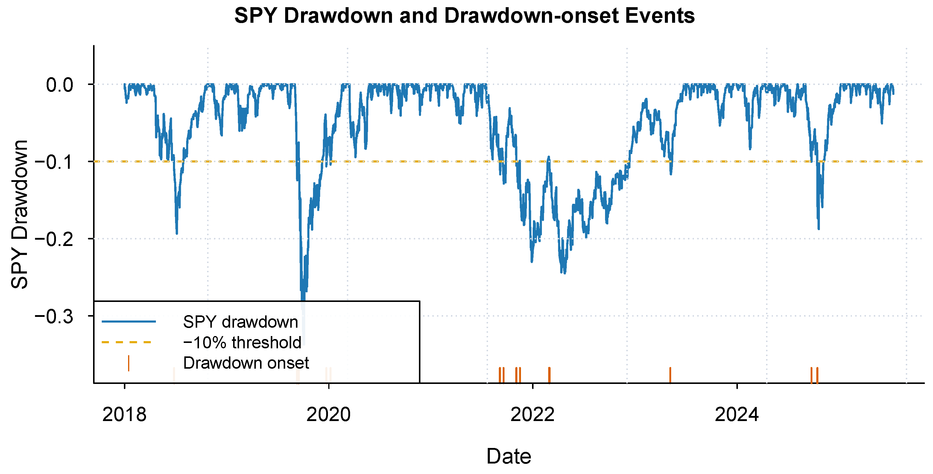
This section first examines whether the leakage-safe residual-stress signal is visually related to subsequent drawdown episodes. Figure 1 reports the residual-stress score, its train-only rolling quantile threshold, and drawdown-onset rug marks. Figure 2 reports the SPY drawdown series, the $-10\%$ drawdown threshold, and the same drawdown-onset rug marks. Rug marks indicate drawdown-onset events, defined as the first entry below the pre-specified drawdown threshold. Residual-stress spikes cluster around several onset dates, indicating that elevated cross-sectional residual dispersion tends to coincide with, and in some episodes precede, transitions into drawdown states. This visual evidence is suggestive rather than conclusive because the modern ETF sample contains only a small number of independent drawdown-onset episodes. In particular, the 2015–2019 subperiod contains only one drawdown-onset event, so subperiod classification metrics and conditional cell estimates should not be interpreted as stable estimates of predictive performance.

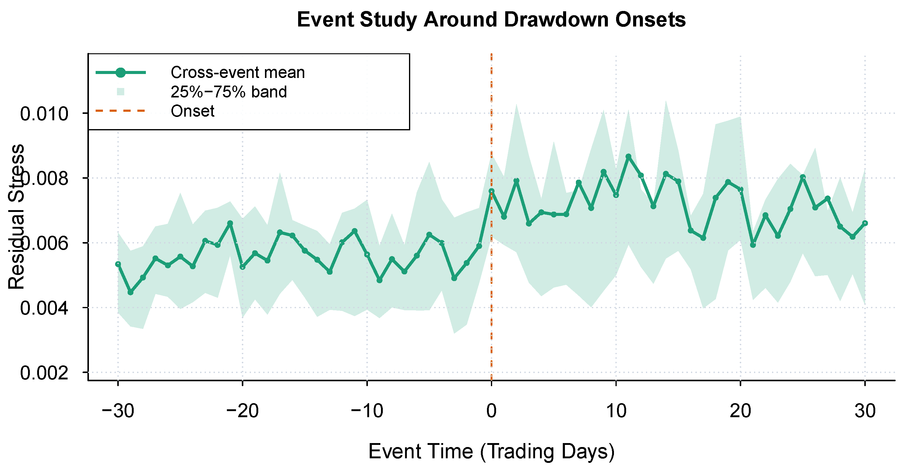
Figure 3 reports an event-study view of the residual-stress score around drawdown onsets. For each onset, days are aligned by event time $\tau$, with $\tau =0$ at the onset, and the cross-event mean stress is computed over the $\pm 30$ trading-day window. The shaded band summarizes cross-event dispersion. Average stress rises around onset episodes, consistent with the interpretation that residual dispersion captures deterioration in cross-sectional market structure during transitions into higher-risk states. However, because drawdown-onset events are rare in the modern ETF sample, this event-study evidence should be interpreted as a descriptive diagnostic rather than conclusive evidence of standalone predictive dominance.

4.2. Early-Warning Evaluation and Benchmark Comparison

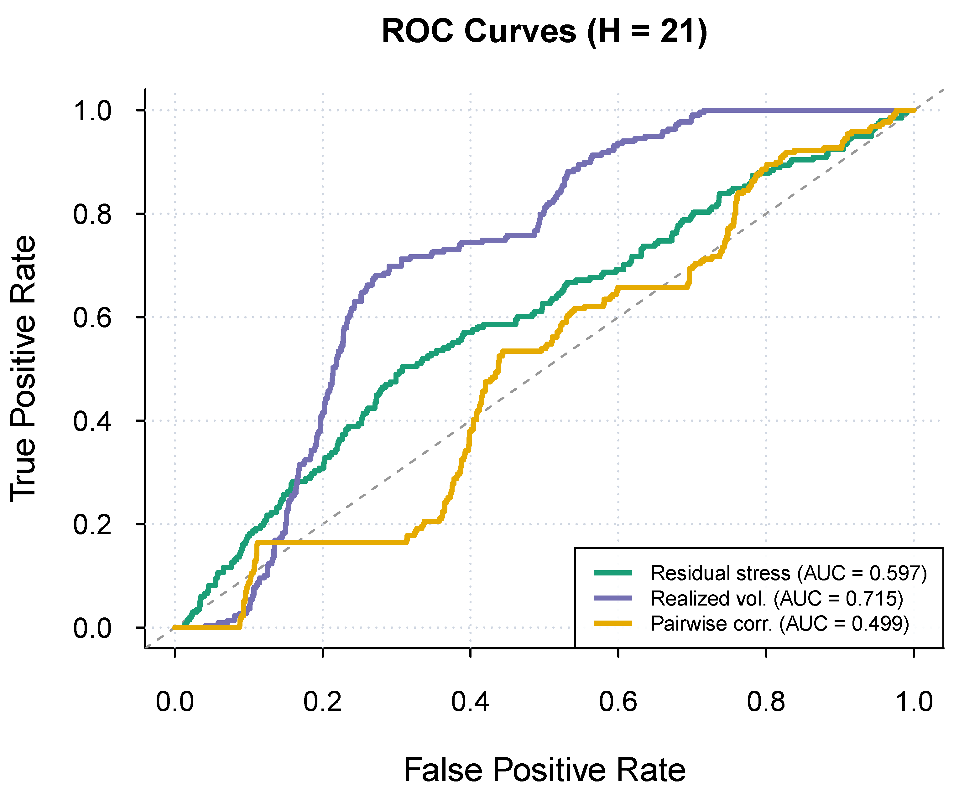
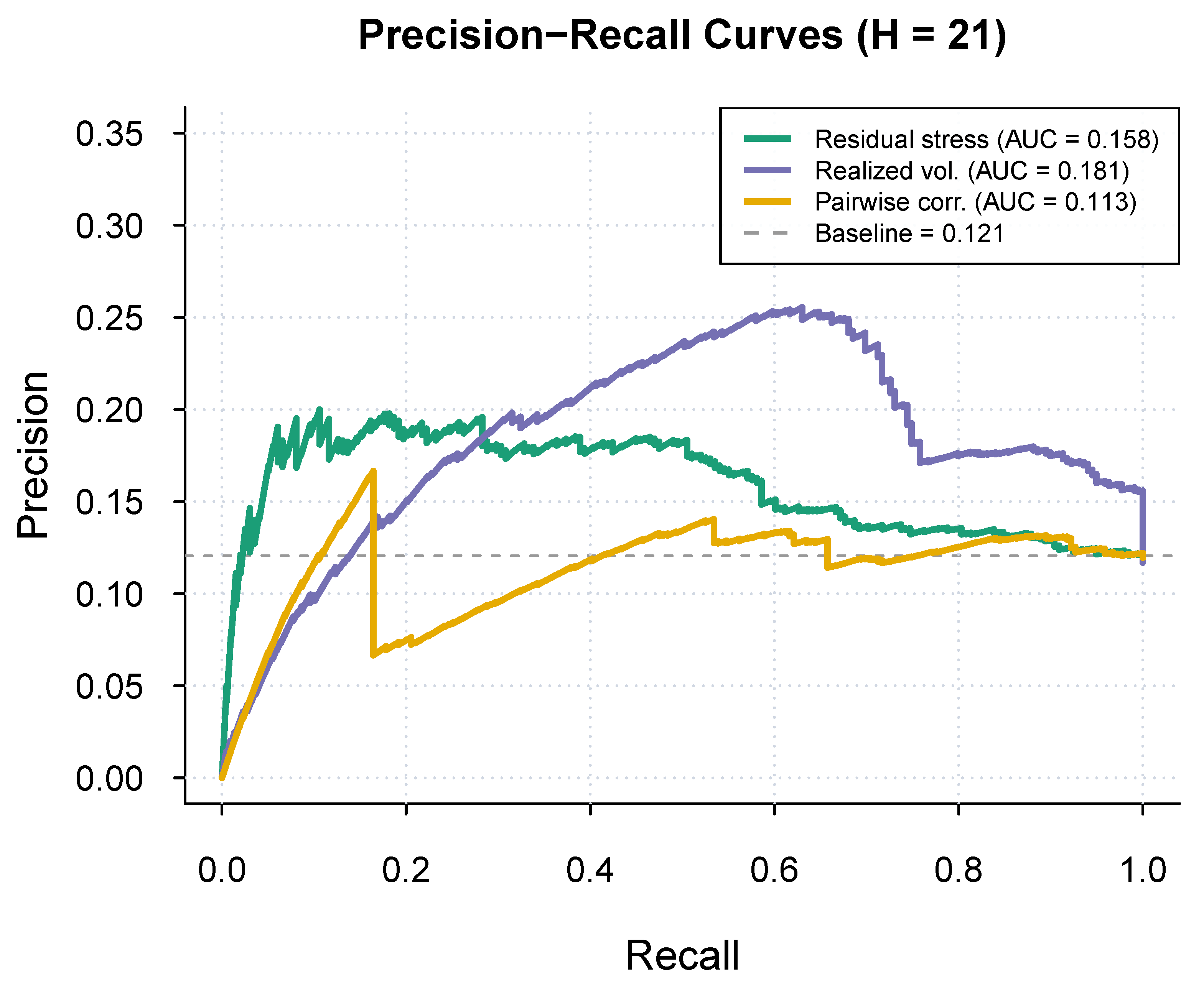
This subsection evaluates whether the residual-stress score contains early-warning information for predicting whether a drawdown onset occurs within the next $H=21$ trading days. Figure 4 reports ROC curves for residual stress, realized volatility, and average pairwise sector correlation. Figure 5 reports the corresponding precision–recall curves. Because drawdown-onset labels are rare, the precision–recall comparison is especially informative. The benchmark comparison shows that residual stress contains positive early-warning information, but realized volatility remains the stronger standalone warning score. In the baseline specification, the unconditional positive-label rate is $\overline{y}=Pr(y_t^{\left(H\right)}=1)\approx 12.1\%$.

Table 1. Leakage-safe early-warning metrics across residual stress and benchmark signals in the main ETF sample.

Signal	ROC-AUC	PR-AUC	Precision	Recall	F1	Event Rate
Residual stress	0.597	0.158	0.233	0.121	0.160	0.121
SPY realized volatility	0.715	0.181	0.263	0.202	0.229	0.117
Avg. pairwise correlation	0.499	0.113	0.035	0.056	0.043	0.120
Cross-sectional dispersion	0.651	0.171	0.212	0.091	0.127	0.116
Downside semivolatility	0.709	0.175	0.331	0.232	0.273	0.117
Breadth	0.462	0.101	0.036	0.010	0.016	0.116
VIX	0.718	0.195	0.321	0.182	0.232	0.116

Notes: Metrics are computed for the horizon-$H=21$ drawdown-onset label with drawdown threshold $\delta =-10\%$. All signals are constructed under the same leakage-safe timing protocol. The VIX row is included when VIX data are available over the relevant sample.

reports aggregate early-warning metrics for residual stress and benchmark signals. Residual stress exhibits nontrivial warning content in the main sample, with ROC-AUC $=0.597$ and PR-AUC $=0.158$. However, realized volatility, downside semivolatility, and the VIX remain stronger standalone benchmarks, with ROC-AUC values of $0.715$, $0.709$, and $0.718$, respectively. Cross-sectional dispersion also performs competitively as a standalone score. Accordingly, residual stress should not be interpreted as a superior standalone classifier. Its more defensible role is as a leakage-safe cross-sectional diagnostic that may contribute conditional and event-level information beyond standard volatility and correlation measures.

The inclusion of rolling average pairwise sector correlation is important because correlation-based measures can rise during stressed markets and may capture broad comovement that overlaps with volatility. In this sample, average pairwise correlation and breadth are weak standalone warning scores, while volatility, VIX, downside semivolatility, and cross-sectional dispersion perform more strongly. Residual stress therefore does not dominate the strongest market-stress benchmarks. Its potential value lies instead in conditional and event-level complementarity.

4.3. Complementarity Relative to Volatility and Correlation

The central empirical question is whether residual stress captures drawdown-risk information not already summarized by standard volatility and correlation measures.

Table 2. Early-warning performance and volatility-complementarity diagnostics in the main ETF sample ($H=21$, $\delta =-10\%$). Panel A reports standalone metrics for residual stress and SPY volatility. Panel B reports joint-regime onset probabilities. Panel C reports event-level overlap within a 63-day lookback window. Panel D reports lead-time diagnostics for paired events.

Panel A: Early-warning metrics for residual stress and volatility.
Signal	ROC-AUC	PR-AUC	Precision	Recall	F1	Event rate
Residual stress	0.597	0.158	0.233	0.121	0.160	0.121
SPY volatility	0.715	0.181	0.263	0.202	0.229	0.117
Panel B: Conditional onset probability by joint regimes.
Regime (Stress, Vol)		N days		$\mathbb{P}\left(\mathrm{onset}\mathrm{within}H\right)$
Low, Low (Q00)		1428		0.1022
High, Low (Q10)		61		0.1967
Low, High (Q01)		110		0.2545
High, High (Q11)		42		0.2857
Panel C: Event-level overlap within a 63-day lookback window.
Category		N events		Share
Both		11		0.786
Stress only		3		0.214
Vol only		0		0.000
Neither		0		0.000
Panel D: Lead time to onset for paired events.
Metric				Value
$n_{\mathrm{paired}}$				11
Median lead, stress				9.0
Median lead, vol				4.0
Mean lead, stress				9.36
Mean lead, vol				18.27
$Pr\left(\mathrm{stress}\mathrm{earlier}\right)$				0.273

separates baseline and complementarity evidence. Panel A reports standalone early-warning metrics for residual stress and SPY volatility, while Panels B–D evaluate whether residual stress adds information through joint-regime conditioning, event-level overlap diagnostics, and lead-time comparisons under the same train-only timing protocol used throughout the paper.

The main-sample evidence is necessarily limited by the small number of drawdown-onset events and the infrequency of high-stress cells. For this reason, the subperiod stability tests, robustness checks, and longer-history proxy-universe evidence are important complements to the main-sample analysis. The role of residual stress is not to replace volatility as a standalone warning score, but to improve risk stratification by contributing conditional and event-level information beyond what is captured by volatility alone.

4.3.1. Joint-Regime Conditioning

Table 2, Panel B, reports the conditional probability of a drawdown onset within the next $H=21$ trading days under the joint regimes defined by residual stress and SPY volatility. Conditional on low volatility, high residual stress increases the onset probability from $10.24\%$ in the low-stress/low-volatility regime to $19.67\%$ in the high-stress/low-volatility regime. The $Q10-Q00$ difference is therefore $9.45$ percentage points. The high-volatility regimes also carry elevated risk, with onset probabilities of $25.45\%$ in the low-stress/high-volatility regime and $28.57\%$ in the high-stress/high-volatility regime. These patterns support the interpretation that residual stress provides complementary conditional information for drawdown-risk stratification, particularly when volatility is not already elevated.

At the same time, the high-stress regimes occur infrequently in the main sample, with $N=61$ and $N=42$ days. The main-sample evidence should therefore be interpreted as suggestive and economically informative rather than as definitive proof of unconditional predictive dominance.

4.3.2. Event-Level Overlap and Lead Time

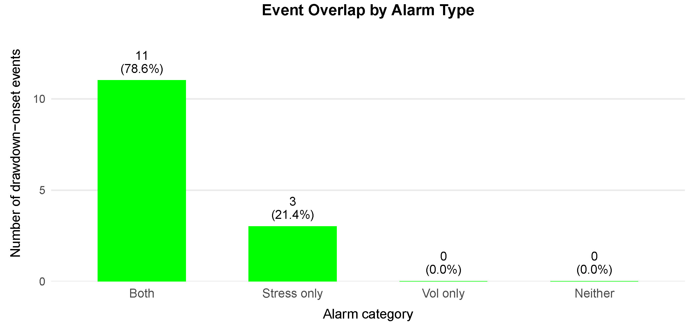
Table 2, Panel C, evaluates whether residual stress flags onset events not captured by volatility thresholding within a fixed 63-trading-day lookback window. In the main sample, both stress and volatility alarms occur within the lookback window before 11 onset events, while residual stress uniquely flags three onset events. Volatility does not uniquely flag any onset event under this rule, and no onset event falls into the neither-alarm category. Table 2, Panel D, reports lead-time diagnostics for paired events in which both alarms occur. Median lead time is nine trading days for stress and four trading days for volatility, while the mean lead time is longer for volatility because of earlier volatility-triggered alarms in some episodes. The stress alarm arrives earlier in $27.3\%$ of paired cases.

Taken together, these results suggest that residual stress contributes partial event differentiation and conditional risk stratification. It is not consistently earlier than volatility, but it can identify some onset episodes that are not captured by a simple volatility-threshold rule. Residual stress therefore appears most useful as a complementary, state-dependent signal rather than as a standalone substitute for volatility.

4.4. Subperiod Stability: 2015–2019, 2020–2025, and 2015–2025

The reviewer concern that the 2020–2025 ETF sample may be unusual is addressed by re-estimating the analysis across three sample windows: 2015–2019, 2020–2025, and 2015–2025. The 2015–2019 period provides a pre-pandemic benchmark, the 2020–2025 period captures a stress-heavy period with major macro-financial shocks, and the full 2015–2025 period evaluates whether the evidence remains stable when both calmer and more turbulent regimes are included.

The 2015–2019 complete 11-sector ETF panel contains only one drawdown-onset event, so ROC-AUC and PR-AUC are not statistically meaningful for that subperiod. This limitation reflects the complete-case ETF universe, especially the shorter histories of XLC and XLRE. In the 2020–2025 and 2015–2025 windows, realized volatility remains the stronger standalone benchmark, while residual stress retains complementary warning content. The purpose of this comparison is not to find a sample window in which residual stress dominates volatility, but to evaluate whether the balanced interpretation remains reasonable across different market environments (see

Table 3. Subperiod stability of residual-stress and volatility early-warning performance.

Sample Window	Onsets	ROC-AUC S	ROC-AUC V	PR-AUC S	PR-AUC V	Main Interpretation
2015–2019	1	–	–	–	–	Too few onsets for reliable classification
2020–2025	14	0.575	0.684	0.162	0.186	Vol stronger; stress complementary
2015–2025	15	0.597	0.715	0.158	0.181	Vol stronger; stress complementary

Notes: S denotes residual stress and V denotes SPY realized volatility. The 2015–2019 row has only one drawdown onset in the complete 11-sector ETF panel, so classification metrics are not reported for that subperiod. All reported metrics use the same leakage-safe timing protocol and the horizon-$H=21$ drawdown-onset label.

).

4.5. Robustness to PCA Window, Factor Selection, and Residual Scaling

The baseline specification uses an expanding-window PCA estimator with fixed $K=2$ and an unscaled RMS residual-stress score. This design is transparent, but it may be sensitive to three modeling choices: the estimation window for PCA loadings, the number of retained principal components, and the fact that the RMS stress score may be influenced by sectors with higher idiosyncratic volatility.

Table 4. Robustness to PCA window, factor-number selection, and residual scaling.

Specification	ROC-AUC	PR-AUC	Precision	Recall	$\mathit{Q}10$–$\mathit{Q}00$	Interpretation
Expanding, $K=2$, unscaled RMS	0.597	0.158	0.233	0.121	0.095	Complementary
Rolling 252, $K=2$	0.580	0.154	0.265	0.131	0.141	Complementary
Rolling 504, $K=2$	0.597	0.161	0.270	0.136	0.141	Complementary
Expanding, $K=2$, idio-vol scaled	0.623	0.182	0.269	0.126	0.123	Complementary

Notes:$Q10$–$Q00$ is the difference in drawdown-onset probability between the high-stress/low-volatility and low-stress/low-volatility regimes. All specifications preserve the same leakage-safe timing protocol.

summarizes robustness checks that address these concerns.

The robustness results show that the complementary interpretation is stable across PCA-window and residual-scaling choices. The idiosyncratic-volatility-scaled version performs best among the residual-stress specifications, with ROC-AUC of $0.623$ and PR-AUC of $0.182$. Rolling-window PCA specifications also preserve positive $Q10$–$Q00$ differences, suggesting that the conditional information in residual stress is not driven solely by the expanding-window baseline.

4.6. Broader-Sample Evidence and Bootstrap Inference

The paper’s central interpretation is evaluated from two complementary empirical views: a modern sector ETF baseline sample and a longer-history proxy-sector sample. The modern sector ETF sample provides the primary contemporary benchmark, but it is short and contains a limited number of drawdown onsets. We therefore pair it with a longer-history proxy-sector universe spanning 1999–2025, which allows a more informative assessment of whether the conditional and event-level role of residual stress is stable across a broader set of drawdown episodes. Moving-block-bootstrap inference and parameter-sensitivity checks are used to quantify sampling uncertainty and assess the robustness of the main interpretation.

4.6.1. Long-History Proxy-Universe Evidence

The longer-history proxy-sector sample provides a broader-event view of the paper’s main interpretation by expanding the analysis to 1999–2025 and increasing the number of drawdown onsets. In this sample, residual stress remains weaker than SPY volatility as a standalone classifier, with ROC-AUC $=0.569$ versus $0.615$ and PR-AUC $=0.108$ versus $0.131$, consistent with the baseline sample. However, the complementary role of residual stress becomes more stable. Conditional on low volatility, high residual stress raises the drawdown-onset probability from $7.72\%$ in the low-stress/low-volatility regime to $15.06\%$ in the high-stress/low-volatility regime, and the bootstrap interval for the $Q10-Q00$ contrast is strictly positive: $0.0735$ with 95% interval $[0.0244,0.1288]$. Event-level diagnostics also strengthen in the broader sample: residual stress uniquely flags seven onset events, volatility uniquely flags none, and the stress alarm arrives earlier in $66.7\%$ of paired cases, with median lead times of 52 trading days for stress versus 40 trading days for volatility. Taken together, the longer-history evidence supports the same substantive conclusion as the modern ETF sample, but with greater event depth and more stable conditional evidence.

4.6.2. Bootstrap Comparison Across Multiple Baselines

Moving-block-bootstrap inference in the modern ETF sample quantifies the uncertainty around the baseline comparisons. The intervals confirm that residual stress contains nontrivial warning content but do not support a claim of standalone dominance over volatility-based benchmarks. Relative to SPY volatility, the bootstrap difference in ROC-AUC is negative. Residual stress nevertheless compares favorably to several weaker auxiliary baselines, including average pairwise correlation and breadth.

Table 5. Summary of baseline and broader-sample evidence for residual-stress complementarity.

Sample	Onsets	ROC-AUC S	ROC-AUC V	PR-AUC S	PR-AUC V	$\mathit{Q}10$–$\mathit{Q}00$	95% CI	S-Only	Pr (S Earlier)
Modern ETF sample	15	0.597	0.715	0.158	0.181	0.095	–	3	0.273
Long-history proxy sample	55	0.569	0.615	0.108	0.131	0.074	[0.024, 0.129]	7	0.667

Notes: S denotes residual stress and V denotes SPY realized volatility. The modern ETF row reports the baseline main-sample values reported earlier in the paper and shown together with Figure 4 and Figure 5. The long-history proxy sample spans 1999–2025. $Q10$–$Q00$ is the difference in onset probability between the high-stress/low-volatility and low-stress/low-volatility regimes. S-only denotes onset episodes uniquely flagged within the event-matching window. Pr (S earlier) is the share of paired events for which residual stress signaled before volatility.

summarizes the baseline and broader-sample evidence for residual-stress complementarity. These results reinforce the paper’s interpretation that the value of residual stress lies in conditional and event-level complementarity rather than in unconditional predictive dominance.

Overall, the bootstrap and broader-sample results support a cautious interpretation. Residual stress is not a superior standalone classifier relative to realized volatility. Its more defensible contribution is that it provides complementary conditional information, especially in states where volatility is not already elevated.

4.7. Economic Performance and Implementation Frictions

As a secondary implementation check, we examine whether the warning signals can be mapped into simple overlay rules after transaction costs. These exercises are not part of the paper’s primary contribution in drawdown-risk monitoring. Instead, they are included to illustrate implementation frictions and to clarify whether information useful for risk-state identification also translates into portfolio decisions.

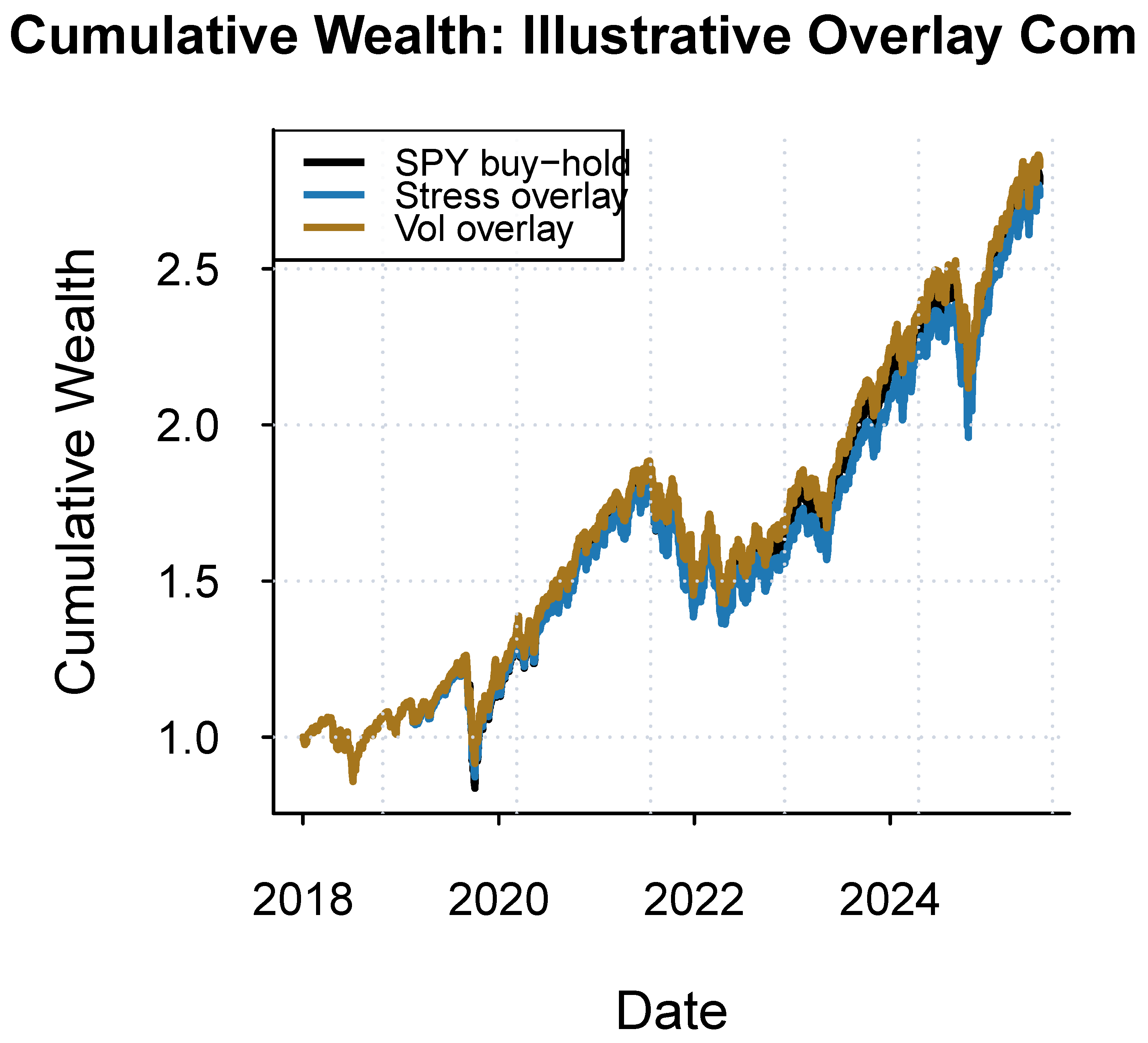
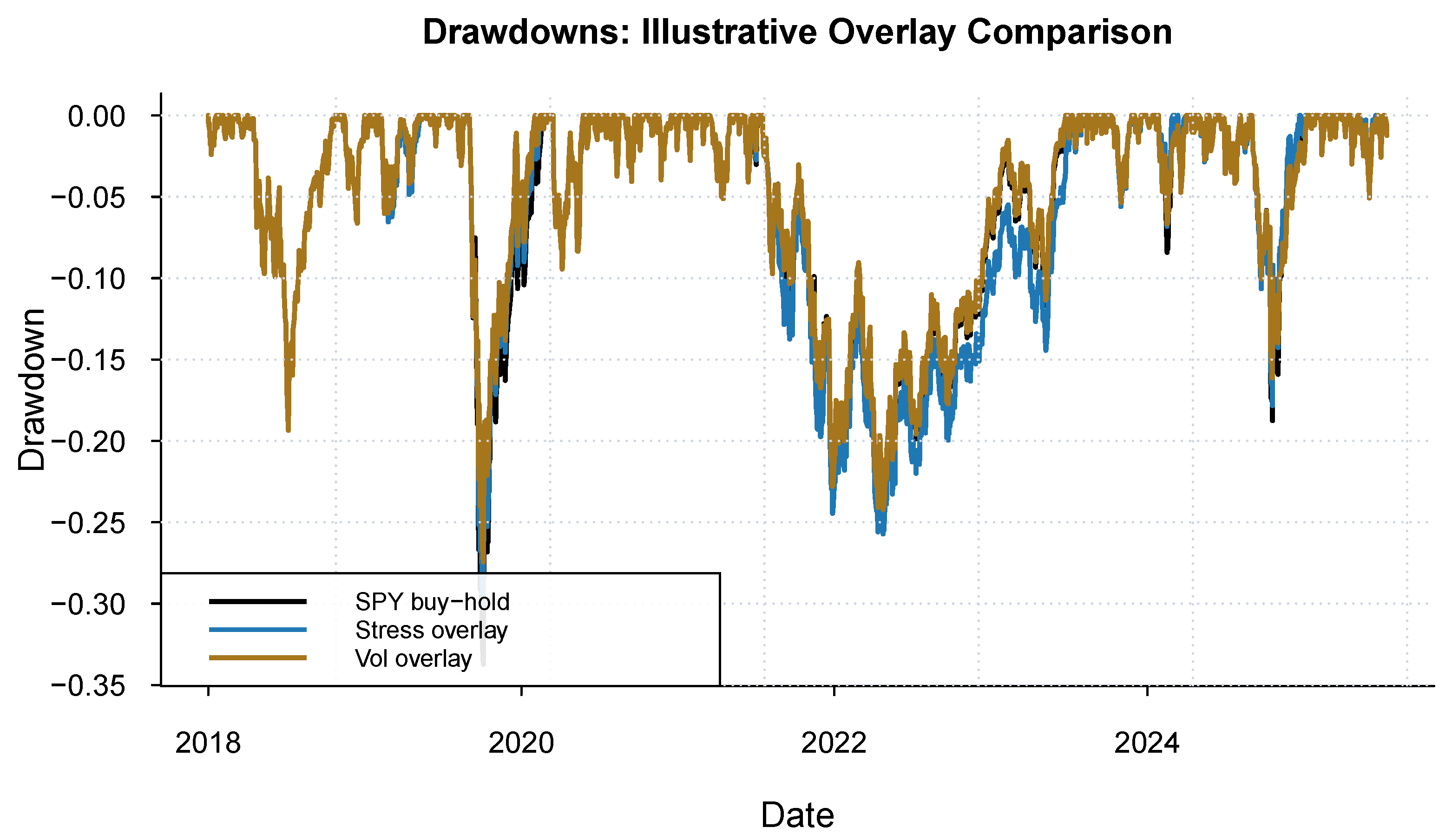
Figure 6 reports cumulative wealth for SPY buy-and-hold returns and two stress-managed SPY overlay variants. Figure 7 shows the corresponding drawdown profiles.

Table 6. Main-sample strategy performance summary under baseline transaction costs.

Strategy	Ann. Return	Ann. Vol	Sharpe	MaxDD
SPY buy-and-hold	0.1458	0.1961	0.7433	−0.3372
SPY overlay, residual stress, 30%	0.1435	0.1826	0.7859	−0.3006
SPY overlay, volatility, 30%	0.1487	0.1747	0.8510	−0.2744

Notes: “Overlay, 30%” denotes scaling risky SPY exposure by $0.7$ when the specified trigger is active, with the remaining $30\%$ held in cash at zero return. Net returns subtract proportional transaction costs of $c=5$ bps per unit of one-way turnover.

summarizes annualized performance over the main sample. The residual-stress overlay slightly reduces annualized return relative to SPY buy-and-hold, but it lowers annualized volatility and improves maximum drawdown. As a result, its Sharpe ratio rises from $0.7433$ for buy-and-hold to $0.7859$. The volatility overlay remains the stronger implementation benchmark, with the highest Sharpe ratio and smallest maximum drawdown. These results support the interpretation that residual stress can be useful as a risk-management overlay, although volatility remains the stronger standalone implementation signal.

Table 7. Transaction-cost sensitivity for the residual-stress overlay.

Cost Assumption	Ann. Return	Ann. Vol	Sharpe	MaxDD
5 bps constant	0.1435	0.1826	0.7859	−0.3006
10 bps constant	0.1400	0.1827	0.7665	−0.3012
25 bps constant	0.1295	0.1828	0.7087	−0.3028

Notes: Transaction costs are proportional costs per unit of one-way turnover. These results evaluate implementation robustness and are not used as the primary evidence for the paper’s contribution.

reports transaction-cost sensitivity for the residual-stress overlay. The transaction-cost scenarios are intended to represent a range of implementation conditions rather than a single precise estimate. The baseline implementation assumes a constant one-way cost of five basis points, intended to approximate a low-friction ETF trading environment. The 10-basis-point case represents a more conservative baseline, while the 25-basis-point case is used as a stressed-cost scenario to reflect wider bid–ask spreads, weaker liquidity, and higher price impact during turbulent periods. These scenarios are motivated by the idea that trading frictions are not constant across market environments and may increase when liquidity provision becomes more costly and market depth deteriorates (Acharya and Pedersen 2005; Amihud 2002; Hasbrouck 2009). They are therefore used as sensitivity checks for implementation robustness rather than as precise estimates of realized execution costs.

Transaction-cost sensitivity confirms that the residual-stress overlay is affected by trading frictions, but the drawdown reduction remains stable across cost assumptions. Under 25 bps constant costs, the Sharpe ratio falls below the buy-and-hold Sharpe ratio, indicating that high frictions can offset the overlay’s risk-management benefit. These results should be interpreted as implementation diagnostics rather than as the paper’s main evidence.

4.8. Descriptive PCA Structure in Sector Excess Returns

For completeness, this subsection summarizes the descriptive PCA structure of the sector excess-return panel. These descriptive results support the use of a parsimonious fixed-$K=2$ baseline, but they are not the main evidence for the paper’s early-warning contribution.

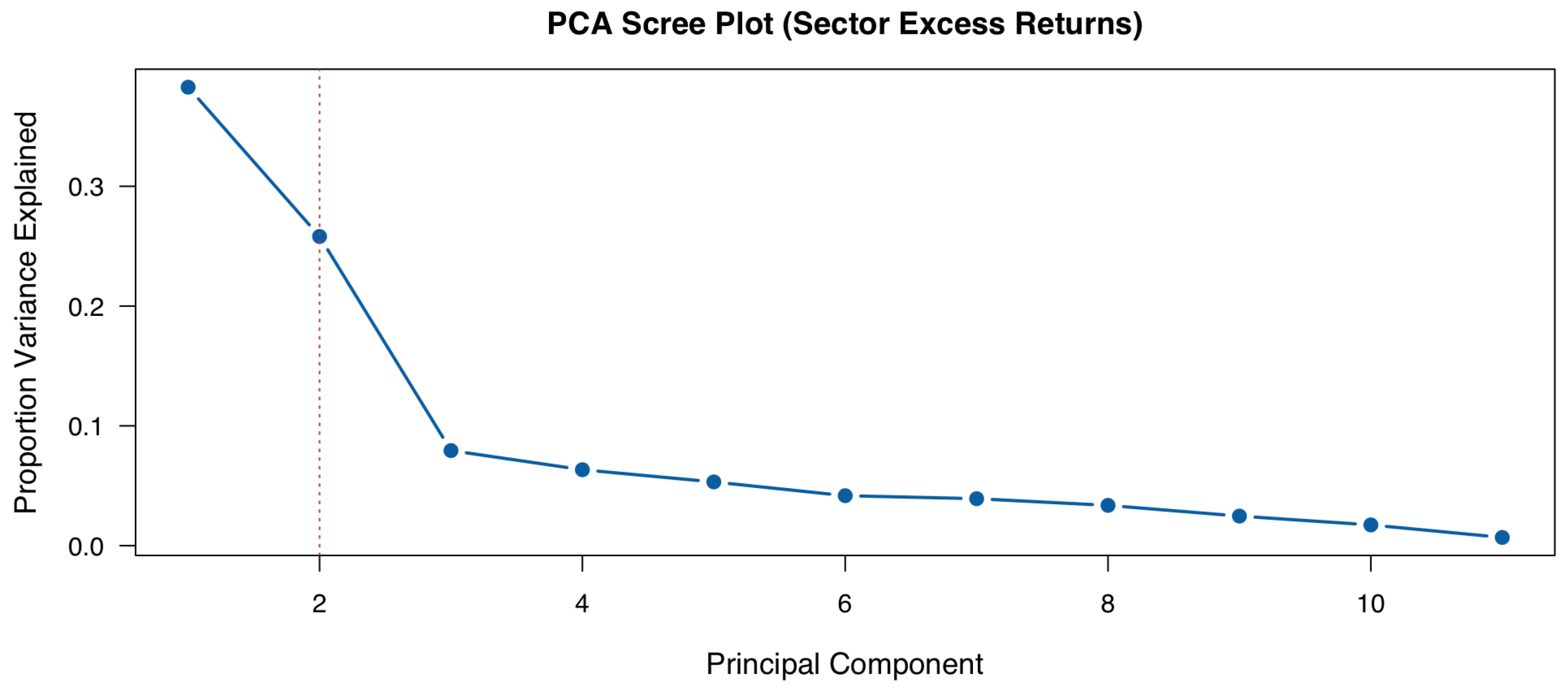
Figure 8 reports the PCA scree plot. In the main sample, the first two principal components explain approximately $64.1\%$ of the cross-sectional variation, supporting the parsimonious baseline choice $K=2$ used throughout the main analysis. Robustness checks above examine whether the conclusions change when the number of retained factors is selected using information criteria of (Bai and Ng 2002).

Table 8. Variance explained by PC1 and PC2 in the main-sample descriptive PCA on sector excess returns.

PC	Explained Variance (%)	Cumulative (%)
PC1	38.27	38.27
PC2	25.81	64.08

reports the variance explained by PC1 and PC2 in the main-sample descriptive PCA.

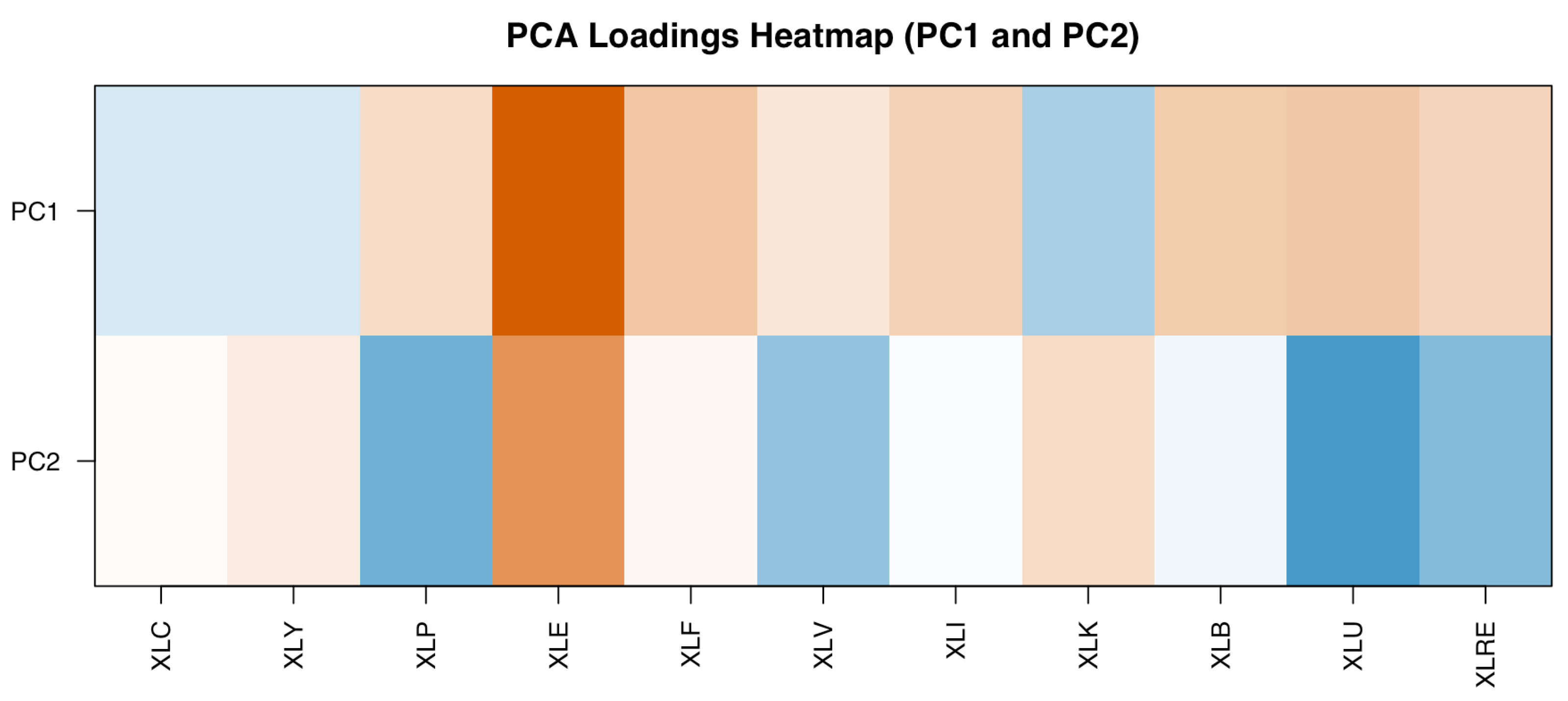
To interpret the economic content of the leading components, Figure 9 displays the PC1–PC2 loading heatmap across the 11 sector ETFs, and

Table 9. Largest absolute PCA loadings for PC1 and PC2 in the main-sample descriptive PCA.

PC	Ticker	Loading
PC1	XLE	0.7611
PC1	XLF	0.2766
PC1	XLU	0.2587
PC1	XLK	−0.2553
PC2	XLU	−0.5413
PC2	XLE	0.5033
PC2	XLP	−0.4233
PC2	XLRE	−0.3652

reports the largest contributors by absolute loading. The heatmap indicates that a low-dimensional factor structure captures much of the common variation in sector excess returns. Differences in sign reflect opposite directional comovement with the corresponding latent component.

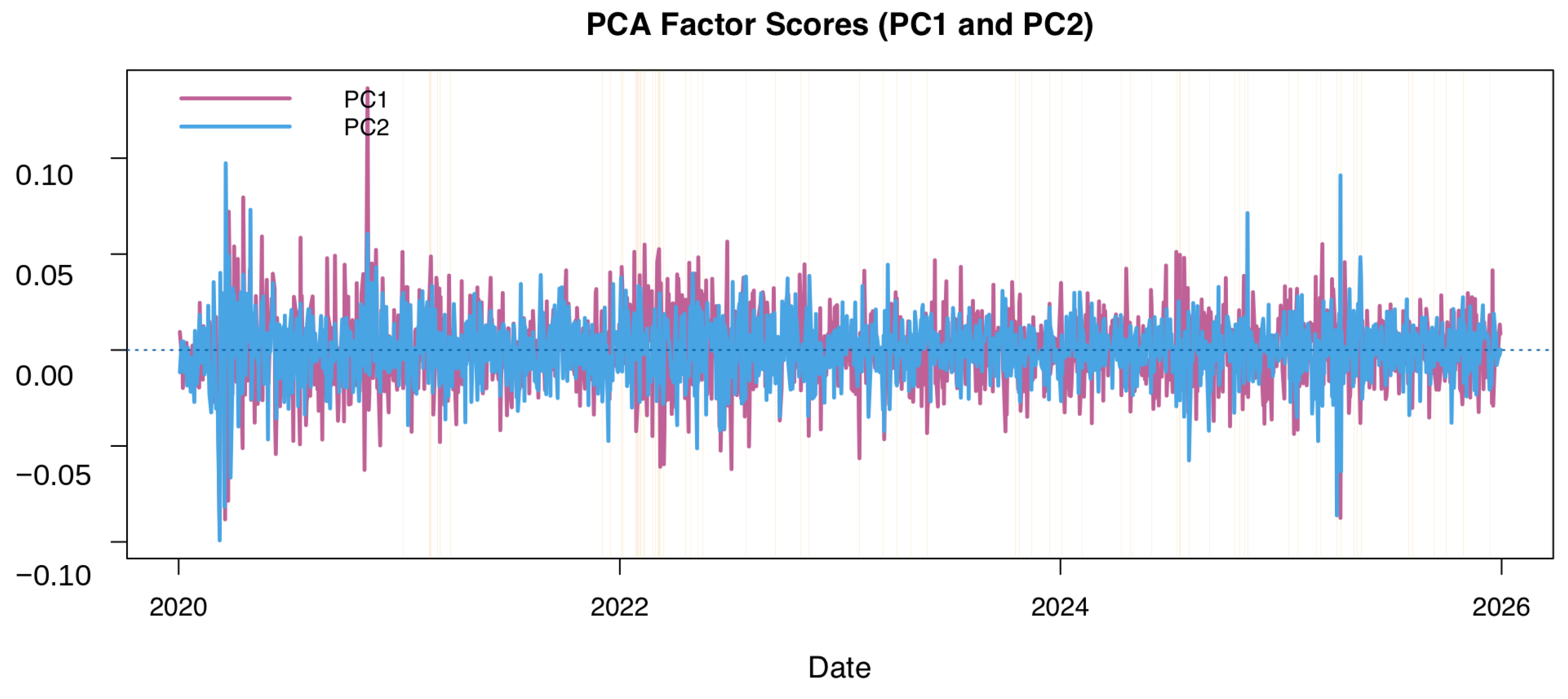
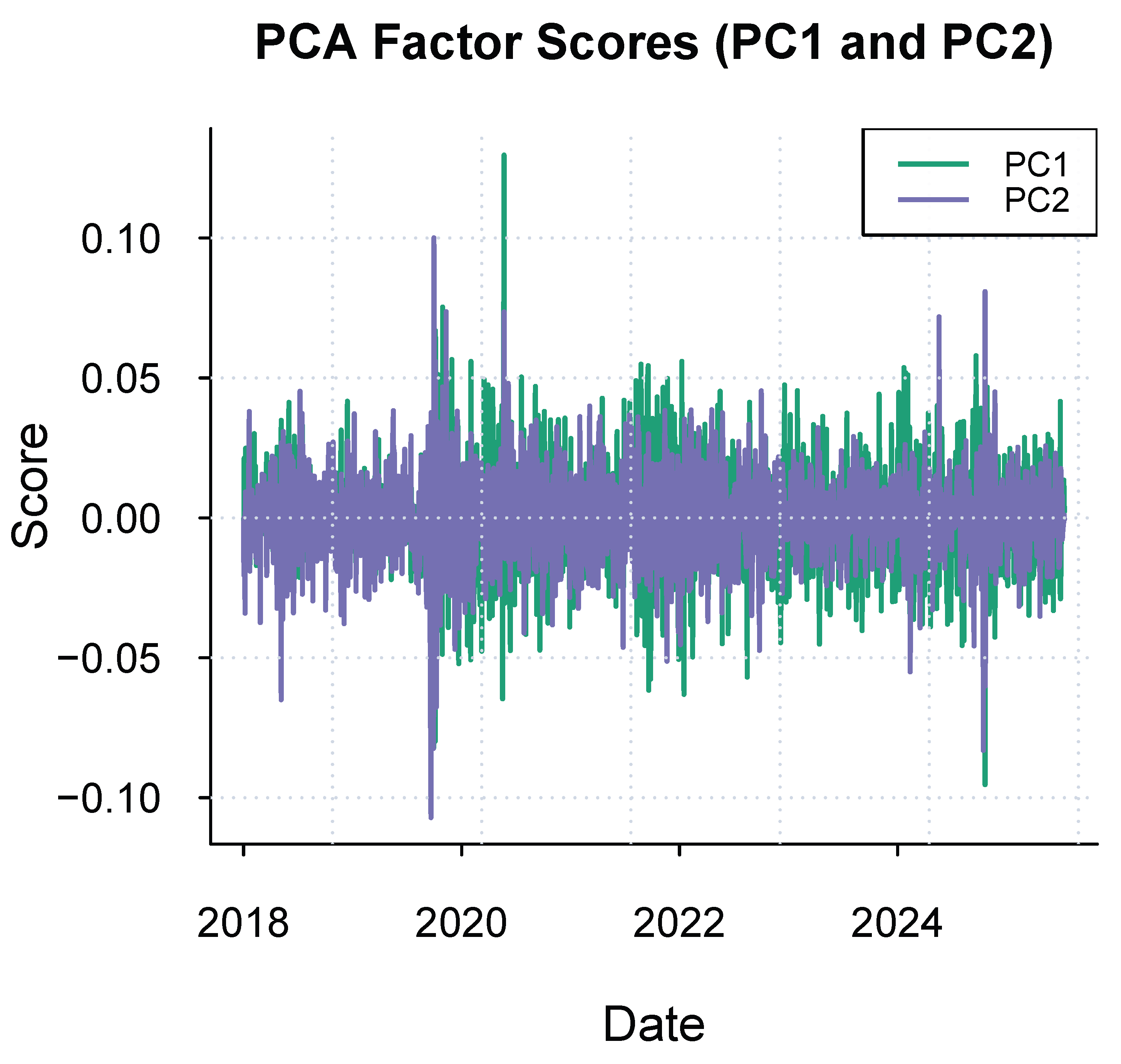
Figure 10 shows that the first two PCA factor scores fluctuate around zero but become more dispersed during several shaded high-stress periods. This pattern is consistent with the interpretation that the common sector structure becomes less stable during market-stress episodes, causing sector excess returns to deviate more strongly from the estimated low-dimensional factor space. However, the figure should be interpreted as descriptive rather than predictive. It supports the use of a parsimonious two-factor representation for visualizing common sector dynamics, while the paper’s main empirical evidence comes from the leakage-safe residual-stress scores, conditional regime analysis, and early-warning tests reported above.

5. Discussion

Realized volatility remains the stronger standalone benchmark in aggregate early-warning metrics, but the results indicate that residual stress contains economically meaningful complementary information in conditional and event-level settings. This study develops a leakage-safe PCA–APT residual-stress index from the cross section of sector excess-return residuals and evaluates its usefulness for monitoring SPY drawdown risk. The main empirical finding is deliberately balanced: residual stress helps characterize cross-sectional market dislocation around drawdown-risk transitions, but it does not dominate realized volatility or the VIX as a standalone classifier. Residual-stress spikes cluster around drawdown onsets (Figure 1 and Figure 3), and the joint-regime evidence in Table 2 indicates that the signal can refine near-term drawdown-risk assessment even when realized volatility remains subdued.

This interpretation is consistent with the paper’s core framing. Volatility captures aggregate time-series fluctuation, whereas residual stress captures fragmentation in the cross section after removal of the dominant common component. It is also useful to distinguish this paper from volatility-forecasting and general machine learning early-warning studies. The aim here is not to improve volatility prediction or to compete primarily on classifier complexity, but to isolate a different information channel—cross-sectional residual fragmentation after removing the dominant sector common component—and to evaluate that channel under an implementable, leakage-safe design. The economic interpretation of the signal is therefore structural and cross-sectional rather than purely time-series- or model-driven.

5.1. Residual Stress as a Drawdown-Risk-Monitoring Signal

The first implication of the results is that cross-sectional residual dispersion appears meaningfully related to transitions into higher-risk market states. Figure 1 shows that large residual-stress spikes tend to cluster around drawdown-onset events, while Figure 3 indicates that average residual stress rises around onset windows. Taken together, these patterns support the interpretation that unusual dispersion in sector-level residual movements is associated with deterioration in market structure during risk-off transitions. Economically, this is plausible: when sectors reprice in a more fragmented or rotational manner, a low-dimensional common-factor structure explains less of the cross section, and the residual component becomes larger. The proposed stress index is designed precisely to capture this type of dislocation.

5.2. Complementary Information Relative to Volatility

The main value of residual stress is not stronger standalone discrimination than volatility, but finer risk stratification in conditional settings. Table 2, Panel A, shows that realized volatility achieves stronger average discrimination than residual stress in the main sample. Panel B, however, indicates that residual stress can still refine drawdown-risk assessment within volatility states. In particular, when volatility is low, moving from the low-stress/low-volatility regime to the high-stress/low-volatility regime raises the probability of a drawdown onset within the next $H=21$ trading days from approximately $10.24\%$ to approximately $19.67\%$. The high-volatility regimes also carry elevated risk, with onset probabilities of approximately $25.45\%$ in the low-stress/high-volatility regime and $28.57\%$ in the high-stress/high-volatility regime. These patterns are consistent with the interpretation that residual stress captures a dimension of cross-sectional fragility not fully summarized by time-series volatility alone.

At the same time, the main-sample evidence should be interpreted with caution. High-stress regimes occur infrequently, and drawdown onsets are rare. Therefore, the conditional-regime results should not be interpreted as definitive proof of unconditional predictive dominance. Instead, they support a narrower and more defensible conclusion: residual stress is best viewed as a complementary monitoring signal whose value is clearer in conditional analysis, event-level diagnostics, and robustness checks than in standalone unconditional classification.

5.3. Residual Stress as a Regime Indicator Rather than a Standalone Return Factor

The empirical results suggest that residual stress should be interpreted primarily as a regime-monitoring variable rather than as a conventional return-prediction factor. The paper’s main evidence comes from drawdown-onset events, regime-conditional probabilities, event-overlap diagnostics, and classification-style warning metrics rather than from strong unconditional average return predictability. This interpretation is appropriate for the problem considered here. Drawdowns are infrequent and nonlinear events, so the value of a signal may lie less in forecasting average returns during normal periods and more in identifying states in which downside-risk management becomes especially relevant. In this sense, the residual-stress index is better viewed as a market-state indicator for monitoring and risk control than as a robust standalone source of alpha.

5.4. Implications for Risk-Management Overlays

The stress-managed SPY overlays illustrate how the signal can be mapped into practical risk-control decisions. In the reported sample, the volatility-based overlay delivers the strongest overall performance, with the highest Sharpe ratio and smallest maximum drawdown. The residual-stress overlay, however, also improves risk-adjusted performance relative to SPY buy-and-hold. Specifically, the residual-stress overlay lowers annualized volatility, improves maximum drawdown from $-0.3372$ to $-0.3006$, and raises the Sharpe ratio from $0.7494$ to $0.7924$ (Table 6). This result supports the interpretation that residual stress can be useful as a practical risk-management overlay, although volatility remains the stronger implementation benchmark.

The transaction-cost sensitivity results provide a more cautious implementation perspective. Under moderate costs, the residual-stress overlay continues to preserve some risk-management benefit, but under a high constant transaction-cost assumption of 25 bps, the Sharpe ratio falls below the buy-and-hold benchmark. This indicates that the value of a residual-stress overlay depends on implementation frictions, threshold design, and trading frequency. The results should therefore be interpreted as implementation diagnostics rather than as the paper’s primary evidence. More refined overlay designs, such as continuous exposure scaling, hysteresis rules, or multi-day confirmation filters, may improve practical performance by reducing unnecessary switching.

5.5. Economic Interpretation of the PCA Factor Space

The descriptive PCA results remain useful for interpretation even though the main contribution of the paper lies in the residual component rather than in the factor scores themselves. Table 8 and Figure 8 show that the first two principal components explain approximately $64.1\%$ of the cross-sectional variation in sector excess returns, supporting the parsimonious baseline choice $K=2$. Figure 9 and Table 9 indicate that a subset of sectors contributes disproportionately to the leading components, consistent with a low-dimensional common structure driven by broad macroeconomic or industry forces. This matters because the stress index is defined relative to that common structure: it measures the extent to which the cross section behaves abnormally after the dominant common component has been removed.

The Bai–Ng robustness check provides an additional perspective on factor-number selection. In the complete ETF panel, the selected factor number is consistently higher than the baseline $K=2$ specification. This selected-K version is less parsimonious and performs somewhat weaker as a residual-stress diagnostic, but it still produces a positive conditional-regime difference. The baseline fixed-$K=2$ specification is therefore retained because it is transparent, interpretable, and economically aligned with the paper’s goal of extracting a dominant common sector structure before measuring residual fragmentation.

5.6. Robustness Considerations and Limitations

The paper reports robustness exercises over subperiods, PCA-window choices, factor-number selection, residual scaling, and transaction-cost assumptions while preserving the same leakage-safe timing protocol throughout. Across these alternatives, the broad qualitative conclusion remains stable: residual stress contains nontrivial warning content and remains associated with drawdown risk, while volatility-based benchmarks remain more competitive in average standalone classification performance. The idiosyncratic-volatility-scaled residual-stress specification performs especially well among the residual-stress variants, suggesting that controlling for sector-specific residual volatility can strengthen the signal.

Several limitations should nevertheless be acknowledged. First, the main results are based on a complete 11-sector ETF panel, and the available sample is constrained by the histories of newer sector ETFs such as XLC and XLRE. As a result, the modern ETF sample contains only a small number of independent drawdown-onset episodes. This limitation is especially important for the 2015–2019 subperiod, which contains only one drawdown-onset event. Therefore, classification metrics and conditional cell estimates in that subperiod should not be interpreted as stable estimates of predictive performance. Second, train-only thresholds, PCA windows, and drawdown definitions involve unavoidable design choices; different choices may alter the frequency and timing of stress labels. Third, because drawdown-onset events are rare by construction, some conditional estimates in Table 2 are based on relatively small cell counts and should therefore be interpreted with caution. Fourth, while the implementation is explicitly designed to be leakage-safe, public market data can still be affected by vendor-specific quirks, symbol changes, and ETF-history limitations.

These considerations do not overturn the main interpretation of residual stress as a complementary monitoring signal. However, they do suggest that the evidence should be interpreted as diagnostic and suggestive rather than conclusive. The empirical contribution is therefore best understood as showing that residual stress provides complementary conditional information for drawdown-risk monitoring, not that it uniformly dominates realized volatility as a standalone early-warning signal. Broader samples, additional markets, and alternative data sources would be useful for establishing external validity more firmly.

5.7. Future Work

Several extensions follow naturally from the present results. First, residual stress could be combined with complementary market-stress variables such as implied volatility, credit spreads, liquidity indicators, or macro-financial uncertainty measures in order to improve joint risk-state detection. Second, the current binary threshold framework could be replaced with a probabilistic mapping from residual stress into drawdown-risk probabilities, for example through walk-forward logistic or hazard-style models. Third, broader validation across other equity universes, international markets, and multi-asset settings would help determine whether cross-sectional residual dispersion is a general indicator of market fragmentation or is more specific to U.S. sector structure. Finally, deeper economic investigation of the mechanisms behind elevated residual stress—such as sector rotation, funding pressure, liquidity shocks, or disagreement shocks—would strengthen the interpretation of the signal and potentially guide more effective overlay design.

6. Conclusions

This paper develops a leakage-safe PCA–APT residual-stress index for equity-market drawdown monitoring using a cross-section of U.S. sector ETFs. The proposed measure is constructed by extracting a low-dimensional common structure from sector excess returns relative to SPY and defining residual stress as the cross-sectional root-mean-square magnitude of the out-of-sample residual component. A train-only rolling quantile rule is then used to convert the continuous stress score into an implementable regime label, allowing drawdown-warning evaluation and illustrative portfolio applications without look-ahead bias.

The paper’s contribution is to develop a leakage-safe, interpretable, cross-sectional residual-stress diagnostic for conditional drawdown-risk monitoring. The results do not support a claim that residual stress dominates realized volatility or the VIX as a standalone early-warning classifier. Realized volatility and the VIX remain stronger unconditional benchmarks in the main early-warning comparisons. Instead, the contribution lies in showing that residual stress provides complementary conditional and event-level information, especially in states where realized volatility is not already elevated.

Empirically, residual-stress spikes cluster around drawdown-onset episodes, and the joint-regime evidence indicates that elevated residual stress is associated with higher near-term drawdown risk even when volatility remains relatively low. In the complete 11-sector ETF sample, moving from the low-stress/low-volatility regime to the high-stress/low-volatility regime nearly doubles the estimated probability of a drawdown onset within the next $H=21$ trading days. Event-overlap diagnostics also show that residual stress flags some onset episodes not captured by a simple volatility-threshold rule. These results support interpreting residual stress as a complementary monitoring signal rather than as a replacement for volatility-based indicators.

Robustness checks further clarify the conditions under which the signal is informative. Rolling-window PCA specifications, Bai–Ng factor-number selection, and idiosyncratic-volatility-scaled residual stress all preserve a positive conditional-regime difference between high-stress/low-volatility and low-stress/low-volatility states. The idiosyncratic-volatility-scaled version performs especially well among the residual-stress variants, suggesting that controlling for sector-specific residual volatility can strengthen the diagnostic value of the signal. At the same time, the 2015–2019 subperiod contains too few drawdown-onset events in the complete ETF panel to support reliable standalone classification metrics, highlighting the importance of broader validation.

The portfolio exercises are best interpreted as implementation diagnostics rather than as a separate source of trading alpha. The stress-managed SPY overlay shows that residual stress can be mapped into a simple risk-control rule that reduces volatility and maximum drawdown relative to buy-and-hold, although the volatility-based overlay remains the stronger implementation benchmark. Transaction-cost sensitivity indicates that high frictions can weaken the overlay’s risk-adjusted performance, so practical use of the signal would likely require careful threshold design, turnover control, and potentially smoother exposure-scaling rules.

Several extensions follow naturally. Future work should evaluate the signal across broader equity universes, international markets, and multi-asset settings; combine residual stress with complementary indicators such as implied volatility, credit spreads, liquidity measures, and macro-financial uncertainty variables; and develop probabilistic drawdown-risk models that map residual stress into calibrated warning probabilities. Additional work on continuous exposure-scaling rules, hysteresis or confirmation filters, turnover-aware overlay design, and external validation would further clarify the practical role of residual-stress indicators in systematic financial risk management. Additional exploratory diagnostics, including the combined-model exercise and related diagnostic figures, are reported in Appendix A.