Short-Term Reversal in Government Bonds: Evidence of State-Dependent Risk from an Emerging Market

Abstract

This study investigates whether short-term reversal exists in an emerging government bond market and whether its returns are consistent with a risk-based explanation. Using Indonesian government bonds from January 2010 to December 2025, the results show that loser portfolios outperform winner portfolios in terms of excess returns relative to the benchmark. A long–short reversal strategy produces statistically significant excess returns and remains highly persistent across rolling 10-year windows, although the evidence is weaker over shorter 5-year horizons. Further analysis indicates that the strategy experiences statistically significant losses during bad times while delivering positive average returns over the full sample, broadly aligned with a risk-based interpretation of short-term reversal. Transaction cost analysis further supports the strategy’s practical feasibility, as observed bid–ask spreads for on-the-run Indonesian government bonds remain below the estimated breakeven threshold. Overall, this study provides rare evidence on short-term reversals, their state-dependent performance, and their practical feasibility in an emerging government bond market.

1. Introduction

Understanding the sources of return predictability is central to asset pricing, as it challenges the efficient market hypothesis (Yen and Lee 2008) and provides insights into why assets earn different returns. From a practical perspective, return predictability is highly relevant to institutional investors seeking to generate portfolio performance that outperforms benchmarks. One such source is short-term reversal, a pattern in which assets that recently underperformed tend to outperform those that previously performed well over short horizons. This effect is typically measured over short evaluation periods, such as one month, enabling the identification of recent under- or overperformance. Extensive evidence documents short-term reversal in equity markets (Jegadeesh 1990; Moskowitz and Grinblatt 1999; Subrahmanyam 2005; Avramov et al. 2006; Butt et al. 2021; Medhat and Schmeling 2022; Dai et al. 2023) and, to a lesser extent, in corporate bond markets (Khang and King 2004; Chordia et al. 2017). More broadly, it is recognized as an investment factor alongside value and momentum (Arnott et al. 2023).

Despite this extensive evidence, empirical findings on short-term reversal in government bond markets remain limited and inconclusive (Khang and King 2004; Zaremba and Czapkiewicz 2017; Zaremba et al. 2019). This gap is particularly striking given that many studies on momentum in global government bonds deliberately exclude the most recent month when constructing 12-month momentum signals (Asness et al. 2013; Ilmanen et al. 2021; Baltussen et al. 2022). Such exclusions reflect concerns about short-term reversals arising from liquidity constraints and market microstructure frictions. Yet, direct empirical evidence on reversal effects in government bond markets remains scarce. As a result, whether short-term reversal represents a systematic and economically meaningful pattern in government bond returns remains an open question.

This question is especially relevant in emerging Asian government bond markets, where return predictability is stronger and shaped by distinct institutional and structural characteristics—such as regulatory quality, governance effectiveness, and market openness—that differ from those in advanced economies, which may contribute to less efficient price discovery processes (Fong and Wu 2020). These features may lead to systematically different return dynamics, underscoring the need for market-specific empirical investigation.

Against this backdrop, this study investigates short-term reversals in the Indonesian government bond market, the largest local-currency government bond market in Southeast Asia by outstanding issuance, according to ADB data (ADB 2025a) and a relatively liquid market (Chernov et al. 2023). Over the past decade, non-resident investors have held between 14% and 40% of tradable government bonds (ADB 2025b), placing Indonesia among emerging markets with the highest levels of foreign participation (IMF 2021). This notable and time-varying foreign presence enhances the analysis’s practical relevance and implies heightened exposure to global risk factors and capital-flow dynamics, making Indonesia a compelling setting for examining short-term reversals.

This study contributes to the literature on asset pricing and factor investing in government bond markets in several ways. First, it provides rare empirical evidence on short-term reversal in an emerging Asian government bond market. Second, it deepens understanding of reversal dynamics by jointly examining their continuousness and persistence and assessing how performance varies across market conditions. Third, it evaluates the practical implementability of reversal strategies by estimating breakeven transaction costs, thereby establishing an upper bound on trading frictions under which the strategy remains competitive relative to a benchmark.

The findings indicate that short-term reversals generate economically meaningful excess returns, exhibit persistence, and are broadly consistent with a risk-based interpretation of reversal profitability. Unlike Zaremba and Czapkiewicz (2017) and Zaremba et al. (2019), who examine reversal using a global cross-country pooling approach, this study investigates cross-maturity reversal dynamics within a single domestic emerging market, namely Indonesia. Similarly, Khang and King (2004) examine both corporate and U.S. Treasury bonds in the United States and find significant reversal effects, primarily in corporate bonds. This study, therefore, helps fill the gap by documenting a reversal in an emerging government bond market and showing that its profitability is state-dependent across good and bad times and remains feasible after accounting for realistic transaction costs.

The remainder of the paper is organized as follows. Section 2 reviews the relevant literature. Section 3 presents empirical results, followed by a discussion of the findings in Section 4. Section 5 describes the data and methods. Section 6 concludes.

2. Literature Review

2.1. Short-Term Reversal: Concepts and Empirical Evidence

Reversal strategies are generally interpreted as mean-reversion strategies, in contrast to momentum strategies that exploit return continuation (Hamdan et al. 2016). Specifically, reversal strategies typically involve taking long positions in previously underperforming assets (losers) and short positions in previously outperforming assets (winners) (Galariotis 2014). Although the construction of reversal signals varies across studies, ranging from weekly (Lo and MacKinlay 1990) to monthly (Jegadeesh 1990) horizons, a one-month formation-and-holding period has become the dominant convention in the literature (Medhat and Schmeling 2022). Shorter horizons may increase signal responsiveness; however, they also increase portfolio turnover and transaction costs, thereby raising important questions regarding the practical implementability of such strategies.

The short-term reversal literature emerged in response to empirical challenges to the weak-form efficient market hypothesis. In a seminal study, Jegadeesh (1990) documented significant negative autocorrelation in monthly stock returns and showed that contrarian strategies could generate abnormal profits. The study further suggested that such return predictability may reflect either market inefficiency or time-varying expected returns.

Subsequent research linked these reversal patterns to market microstructure frictions, particularly bid–ask bounce effects that can mechanically generate negative serial correlation in observed returns (Conrad et al. 1997). Later studies, however, suggest that reversal cannot be fully explained by microstructure mechanisms alone. Subrahmanyam (2005), for example, shows that reversal effects remain significant even when returns are estimated using mid-point quotes, weakening the argument that reversal merely reflects bid–ask bounce effects. Short-term stock return reversals are more likely driven by investor overreaction and belief reversion than by inventory effects. More recent evidence further indicates that reversal dynamics depend on trading characteristics. Butt et al. (2021) document that reversals tend to be stronger for small-cap and highly volatile assets. Meanwhile, Medhat and Schmeling (2022) show that reversal patterns are closely related to trading intensity: stronger reversals are concentrated among low-turnover assets, whereas highly traded assets tend to exhibit short-term momentum. Accordingly, the short-term reversal literature has evolved from viewing reversal primarily as a mechanical consequence of bid–ask bounce and market inefficiency toward a broader interpretation in which reversal reflects the interaction among firm characteristics, liquidity conditions, trading activity, and investor behavior. The existing literature has primarily focused on behavioral and market microstructure explanations, while paying relatively little attention to the risk-based perspective.

2.2. Short-Term Reversal in Bond Markets

Evidence of reversal subsequently extended to the corporate bond market, where several studies suggest that reversal is more closely related to liquidity provision and market microstructure frictions. Khang and King (2004), for example, conclude that short-term reversals in U.S. corporate bonds are primarily driven by dealer inventory effects and market microstructure frictions. These findings are consistent with the view that reversals in corporate bond markets are more closely related to liquidity-provision mechanisms than to investor overreaction. Consistent with this interpretation, Chordia et al. (2017) show that the profitability of monthly reversal strategies in corporate bonds is significantly related to a proxy for illiquidity, supporting the view that reversal partly compensates for liquidity provision.

Early evidence from the U.S. Treasury markets found no support for short-term reversal (Khang and King 2004), and cross-country studies similarly reported weak or absent reversal effects (Zaremba and Czapkiewicz 2017; Zaremba et al. 2019). Kassimatis et al. (2008) documented a reversal in international government bond markets; however, this evidence was event-driven, occurring only following market shocks. Taken together, these results contrast with the robust findings in equity and corporate bond markets, leaving the existence of short-term reversals in government bond markets—and their practical implementability net of transaction costs—open empirical questions. This contrast is particularly interesting given that both corporate and government bond markets operate through dealer-based market structures.

2.3. Risk-Based Interpretation of Short-Term Reversal

The existing literature on short-term reversal has generally evolved into two main explanations: behavioral explanations and market microstructure-based explanations (Aghassi et al. 2023). The behavioral literature argues that reversals reflect investor overreaction or belief-revision errors, in which prices temporarily deviate from fundamental values as investors respond excessively to information before prices eventually correct (Subrahmanyam 2005). From a market microstructure perspective, reversal is viewed as a consequence of trading frictions and liquidity provision. Dealers or liquidity providers bear inventory risk when facing temporary order imbalances, which can put prices under pressure before they subsequently readjust (Jegadeesh and Titman 1995). More recent studies further suggest that reversal may represent compensation for liquidity provision, particularly during periods of heightened market volatility and tighter funding conditions (Butt et al. 2021). In addition, Dai et al. (2023) show that volatility and trading turnover influence the strength and persistence of reversal through the inventory risk and inventory duration borne by liquidity providers. Taken together, the existing literature suggests that short-term reversal may arise not from a single mechanism, but rather from the interaction among market frictions, liquidity conditions, trading activity, and investor behavior.

Despite these advances, existing studies in the reversal literature have generally focused on market microstructure and liquidity-based explanations, with relatively limited attention to broader risk-based interpretations. From a risk-based perspective, short-term reversal strategies may be particularly vulnerable during adverse states, when persistent price pressures and weakened mean reversion amplify downside risk (Hamdan et al. 2016). In such environments, deviations from fundamental values may widen rather than revert, increasing the likelihood of losses. This interpretation suggests that short-term reversals may reflect not only behavioral or microstructure-driven phenomena, but also compensation for exposure to adverse market states. Within this framework, factor premia are viewed as compensation for exposure to assets that perform poorly during adverse economic conditions, often referred to as “bad times” (Ang 2014).

Ang (2014) argues that the factor premium represents compensation for investors willing to bear losses during such adverse periods. Analytically, if a factor never performs poorly when investors most urgently need liquidity, namely during periods of high marginal utility, it will not offer high expected returns in the future. Accordingly, true risk is not merely nominal volatility but the possibility of poor performance occurring precisely during the periods most painful for investors.

2.4. Bad Times and the Consumption-Based Asset Pricing Framework

The notion of bad times emphasized by Ang (2014) is closely rooted in the consumption-based asset pricing framework. Within the Consumption-Based Capital Asset Pricing Model (CCAPM), Breeden (1979) argues that asset risk should be evaluated in terms of the relationship between asset returns and aggregate consumption growth. Assets that perform poorly during periods of declining consumption are considered particularly risky because they generate losses precisely when investors face the highest marginal utility of wealth and therefore require economic resources most urgently. Consequently, such assets must offer higher expected returns as compensation for bearing adverse consumption risk.

Consistent with this framework, Ang (2014) explicitly defines bad times as states in which aggregate consumption deteriorates and marginal utility rises sharply. In such environments, even small losses become economically painful for investors because each additional unit of wealth becomes increasingly valuable. From this perspective, true investment risk is not merely reflected in unconditional volatility but in an asset’s or factor’s tendency to perform poorly during bad times. Operationally, however, the notion of bad times has evolved beyond purely consumption-based contractions and is frequently extended to broader episodes of macro-financial stress, including a slowing economy, elevated market volatility, inflationary pressures, deteriorating liquidity, and severe asset price declines.

Gormsen and Greenwood (2017) similarly acknowledge that the concept of bad times originates in the consumption-based asset-pricing tradition. Although they recognize that consumption-based measures alone often face empirical limitations in fully explaining asset prices, they nevertheless preserve the normative implication of the CCAPM framework: investors should dislike assets that perform poorly during adverse states of the world. Extending this logic, they operationalize bad times as periods during which economic and financial distress co-occur. Financial bad times are empirically identified when excess stock market returns fall within the lowest historical quintile, whereas economic bad times are identified using the NBER recession indicators. They characterize “rainy days,” or bad times, as periods of broad-based deterioration associated with large negative excess stock market returns, economic contraction, declining corporate earnings, elevated inflation and unemployment, and falling housing prices. This joint-state framework is designed to minimize false positives and ensure that bad times capture genuinely adverse macro-financial conditions that investors face.

However, the empirical operationalization of bad times in their study relies primarily on broad stock market proxies and developed-market macroeconomic indicators. Applying this framework to emerging-market government bond markets requires several contextual adjustments. In Indonesia, for example, important constraints include the difficulty of measuring financial-market distress, the rarity of technical recessions, the unavailability of housing-market data, and the low frequency of unemployment statistics, which are published only biannually.

2.5. Hypothesis Development

The analysis evaluates short-term reversal through three dimensions—continuousness, persistence, and consistency—following Coche et al. (2018). Continuousness assesses whether stronger reversal signals systematically translate into higher subsequent returns, implying that long–short strategies that buy prior losers and sell prior winners generate positive excess returns. The prior literature from corporate bond markets suggests several mechanisms through which reversal may arise. These include temporary price pressure, liquidity provision, and dealer inventory adjustment, all of which may cause prices to temporarily deviate from fundamental values before subsequently reverting (Khang and King 2004; Chordia et al. 2017). Consequently, assets facing temporary selling pressure become underpriced, generating a reversal effect as prices subsequently revert to fundamental values. If continuousness holds, stronger price pressure should lead to stronger subsequent reversals, rewarding a long-short strategy. Accordingly, the following hypothesis is proposed:

H1: 

The short-term reversal strategy yields positive average excess returns.

Persistence examines whether such performance remains stable over time and across varying market conditions. If reversal reflects recurring structural frictions—such as dealer inventory adjustment and liquidity provision—rather than isolated market anomalies, its profitability should persist over time as a stable compensation mechanism. Therefore, the following hypothesis is proposed:

H2: 

The short-term reversal strategy exhibits temporal persistence.

Consistency evaluates whether reversal performance aligns with theoretical expectations from a risk-based perspective. Consistent with the theoretical discussion in the literature review, the CCAPM framework suggests that factor premia represent compensation for bearing losses during adverse economic and financial conditions, commonly referred to as bad times. In normal market conditions, reversal strategies profit from temporary price pressure and subsequent mean reversion. However, during bad times—when investors face declining consumption and high marginal utility of wealth—liquidity conditions deteriorate, and selling pressure persists. In such environments, prior losers continue to underperform, effectively weakening the normal mean-reversion mechanism. Therefore, the following hypothesis is proposed:

H3: 

The short-term reversal strategy weakens (underperforms) during bad times.

3. Results

3.1. Descriptive Statistics

Table 1. Descriptive Statistics of Excess Returns, Standard Deviations, and Durations.

Maturity	Average	Standard Deviation	Average Duration
5-year bond	2.06%	5.23%	4.09
10-year bond	3.34%	8.62%	7.00
15-year bond	4.18%	10.11%	8.97
20-year bond	5.22%	11.28%	10.15

Note: Mean denotes the average monthly excess return for each maturity segment. All reported means and standard deviations are annualized. Means are multiplied by 12, and standard deviations are multiplied by $\sqrt{12}$. Average duration represents the average bond duration within each maturity segment. All figures are rounded to 2 decimal places. The sample consists of 768 return observations (4 bonds × 192 months). The sample period spans January 2010 to December 2025.

reports the average excess returns, standard deviations, and average durations across maturity segments in the Indonesian government bond market over the sample period. The results show that average excess returns increase with maturity. The 5-year bond segment records an average excess return of 2.06%, while the 20-year bond segment records the highest average excess return at 5.22%. A similar pattern is observed for return volatility, which rises from 5.23% for 5-year bonds to 11.28% for 20-year bonds. Average duration also increases across maturity segments, ranging from 4.09 years for the 5-year bonds to 10.15 years for the 20-year bonds.

3.2. Short-Term Reversal Across Signal Ranks and Maturities

Table 2. Excess Returns, Standard Deviations, Sharpe Ratios, and Durations by Signal-Based Rank.

Statistics	B1 (Best)	B2	B3	B4 (Worst)	Benchmark
Mean (t-stat)	1.27% (0.58)	3.13% (1.33)	4.25% (1.84) *	6.15% (2.73) ***	3.70% (1.75) *
Standard deviation	8.71%	9.39%	9.24%	9.01%	8.46%
Sharpe ratio	0.15	0.33	0.46	0.68	0.44
Average duration	7.13	7.64	8.04	7.40	7.55

Note: Mean (t-stat) denotes the average excess return for each rank, with t-statistics reported in parentheses. Reported means, standard deviations, and Sharpe ratios are annualized. Average duration represents the average bond duration within each rank. All figures are rounded to two decimal places. Statistical significance is denoted by *** p < 0.01, * p < 0.10.

presents mean excess returns, standard deviations, Sharpe ratios, and average durations for government bonds ranked by the short-term reversal signal, from B1 (best past performance) to B4 (worst past performance). The sorting procedure reveals a monotonic increase in the point estimates of average excess returns. Moving from B1 to B4, the mean excess return rises from 1.27% to 6.15%. An examination of the statistical significance of individual bonds reveals an important asymmetry in the reversal effect: the excess returns of B4 are statistically significant at the 1% level (t = 2.73), whereas the excess returns of B1 and B2 are statistically indistinguishable from zero (t = 0.58).

The standard deviations are relatively stable across all bonds, ranging from 8.71% to 9.39%. Given this broadly similar level of volatility, the B4 bond’s higher mean excess return translates into stronger risk-adjusted performance in economic terms. Consistent with this pattern, the point estimate of the Sharpe ratio, a descriptive metric, increases monotonically from 0.15 for B1 to 0.68 for B4, exceeding the benchmark of 0.44. Because the mean excess return of B1 is not statistically different from zero, the economic relevance of its estimated risk-adjusted performance appears relatively weak compared with the B4 bond.

To examine the distribution of signal ranks across maturities,

Table 3. Average Bond Ranks by Maturity.

Statistics	5-Year Bond	10-Year Bond	15-Year Bond	20-Year Bond
Average rank	2.42	2.45	2.56	2.57

Note: Average ranks are calculated monthly over the sample period for each maturity (5-, 10-, 15-, and 20-year). All figures are rounded to two decimal places.

reports the average bond ranks for each maturity segment. Each month, bonds are sorted based on the short-term reversal signal and assigned ranks from 1 (highest signal) to 4 (lowest signal). The results indicate that signal-based bond ranks are relatively evenly distributed across maturities, and the Friedman test detects no statistically significant differences along the yield curve.

As reported in

Table 4. Duration-Adjusted Excess Returns, Standard Deviations, and Sharpe Ratios by Duration-Adjusted Signal-Based Rank.

Statistics	B1 (Best)	B2	B3	B4 (Worst)	Benchmark
Mean (t-stat)	0.29% (0.97)	0.52% (1.77) *	0.54% (1.77) *	0.77% (2.49) **	0.53% (1.84) *
Standard deviation	1.19%	1.18%	1.21%	1.23%	1.15%
Sharpe ratio	0.24	0.44	0.44	0.62	0.46

Note: Mean (t-stat) denotes the average duration-adjusted excess return for each rank, with t-statistics reported in parentheses. Reported means, standard deviations, and Sharpe ratios are annualized. All figures are rounded to two decimal places. Statistical significance is denoted by ** p < 0.05, * p < 0.10.

, applying the duration adjustment yields a systematic improvement in the point estimates of average excess returns. Moving from B1 to B4, the mean duration-adjusted excess return increases from 0.29% to 0.77%. Statistical testing indicates that the duration-adjusted returns of B4 are significant at the 5% level (t = 2.49), whereas the returns of B1 are statistically indistinguishable from zero (t = 0.97). Regarding volatility, the standard deviations do not exhibit a strict monotonic pattern. The point estimates for B3 (1.21%) and B4 (1.23%) are nominally higher than those for B1 (1.19%) and B2 (1.18%), though all remain constrained within a narrow range. Correspondingly, the point estimate of the Sharpe ratio increases from 0.24 for B1 to 0.62 for B4, exceeding the benchmark’s 0.46.

3.3. Loser Portfolios Outperform Winner and Benchmark Portfolios

Table 5. Signal-Based Portfolio Performance.

Statistics	P1 (Winner)	P2 (Loser)	Factor (Long Short)	Benchmark
Mean (t-stat)	2.20% (1.01)	5.20% (2.37) **	3.94% (3.00) ***	3.70% (1.75) *
Standard deviation	8.67%	8.76%	5.26%	8.46%
Sharpe ratio	0.25	0.59	0.75	0.44
Alpha (t-stat)	−1.48% (−2.67) ***	1.48% (2.67) ***	3.89% (2.93) ***
Average duration	7.72	7.38		7.55

Note: Mean (t-stat) denotes the average excess returns, with t-statistics reported in parentheses. Reported means, standard deviations, Sharpe ratios, and alphas are annualized. All series are found to be stationary at the 1% significance level based on the ADF test. Alpha (intercept) is estimated relative to the benchmark using the Newey–West t-statistics. All figures are rounded to two decimal places. Statistical significance is denoted by *** p < 0.01, ** p < 0.05, * p < 0.10.

reports the performance of portfolios constructed using the short-term reversal signal: the winner portfolio (P1), the loser portfolio (P2), the factor portfolio, and the benchmark portfolio. The performance metrics show that P2 generates a mean return of 5.20% that is statistically significant at the 5% level (t = 2.37). In contrast, P1 yields a lower mean return of 2.20%, which is statistically indistinguishable from zero (t = 1.01). However, the difference between the two is not statistically distinguishable from zero. After controlling for broad market movements, P2 delivers a positive and statistically significant estimated alpha of 1.48% (t = 2.67), whereas P1 exhibits a negative alpha of −1.48% (t = −2.67).

In terms of interest-rate exposure, P2 has an average duration of 7.38, compared with 7.55 for the benchmark and 7.72 for P1. The differences in duration between the benchmark and both the winner and loser portfolios are not statistically significant.

For the factor portfolio, the mean excess return is 3.94% (t = 3.00), compared with 3.70% for the benchmark (t = 1.75). The factor portfolio also records a lower standard deviation of 5.26%, compared with 8.46% for the benchmark, and a higher point estimate of the Sharpe ratio (0.75 versus 0.44 for the benchmark). Finally, the factor portfolio delivers a positive and statistically significant alpha of 3.89% (t = 2.93).

Table 6. Duration-Adjusted Signal-Based Portfolio Performance.

Statistics	P1 (Winner)	P2 (Loser)	Factor (Long Short)	Benchmark
Mean (t-stat)	0.40% (1.41)	0.65% (2.20) **	0.36% (2.92) ***	0.53% (1.84) *
Standard deviation	1.15%	1.19%	0.50%	1.15%
Sharpe ratio	0.35	0.55	0.73	0.46
Alpha (t-stat)	−0.12% (−2.07) **	0.12% (2.07) **	0.35% (2.77) ***

Note: Mean (t-stat) denotes the average duration-adjusted excess return, with t-statistics reported in parentheses. Reported means, standard deviations, Sharpe ratios, and alphas are annualized. Alpha (intercept) is estimated relative to the benchmark. All series are found to have no autocorrelation or heteroscedasticity and to be stationary at the 1% significance level based on the ADF test. All figures are rounded to two decimal places. Statistical significance is denoted by *** p < 0.01, ** p < 0.05, * p < 0.10.

presents a robustness check using portfolios constructed with the duration-adjusted reversal signal to assess whether the signal-based portfolio performance persists after controlling for duration risk. The duration-adjusted performance metrics indicate that P2 generates a statistically significant mean duration-adjusted excess return of 0.65% (t = 2.20). In contrast, P1 yields a lower mean return of 0.40% that is statistically indistinguishable from zero (t = 1.41). In terms of duration-adjusted benchmark comparisons, P2 delivers a positive, statistically significant alpha of 0.12% (t = 2.07), whereas P1 exhibits a negative, statistically significant alpha of −0.12% (t = −2.07).

For the duration-neutral factor portfolio, the duration-adjusted mean return remains statistically significant at 0.36% (t = 2.92). Because the long–short construction neutralizes much of the residual volatility, the factor portfolio records a markedly lower standard deviation of 0.50%, compared with 1.15% for the benchmark. This volatility reduction leads to a higher point estimate of the Sharpe ratio (0.73) than the benchmark (0.46). Most importantly, the factor portfolio delivers a positive and statistically significant alpha of 0.35% (t = 2.77).

3.4. Factor Performance Exhibits Long-Term Persistence

The temporal stability of the factor strategy is evaluated using success ratios across rolling windows, as detailed in

Table 7. Success Ratios of Factor Portfolio Performance across Rolling Windows.

Statistics	5 Years	10 Years
Success ratio (%)	60.90	95.89
Number of windows	133	73

Note: “Success” is defined as a positive and statistically significant excess return at the 5% level within the window. All figures are rounded to two decimal places.

. The results show a 95.89% success rate over the 10-year window, confirming strong persistence over the 16-year sample period, but a lower 60.90% success rate over the 5-year window.

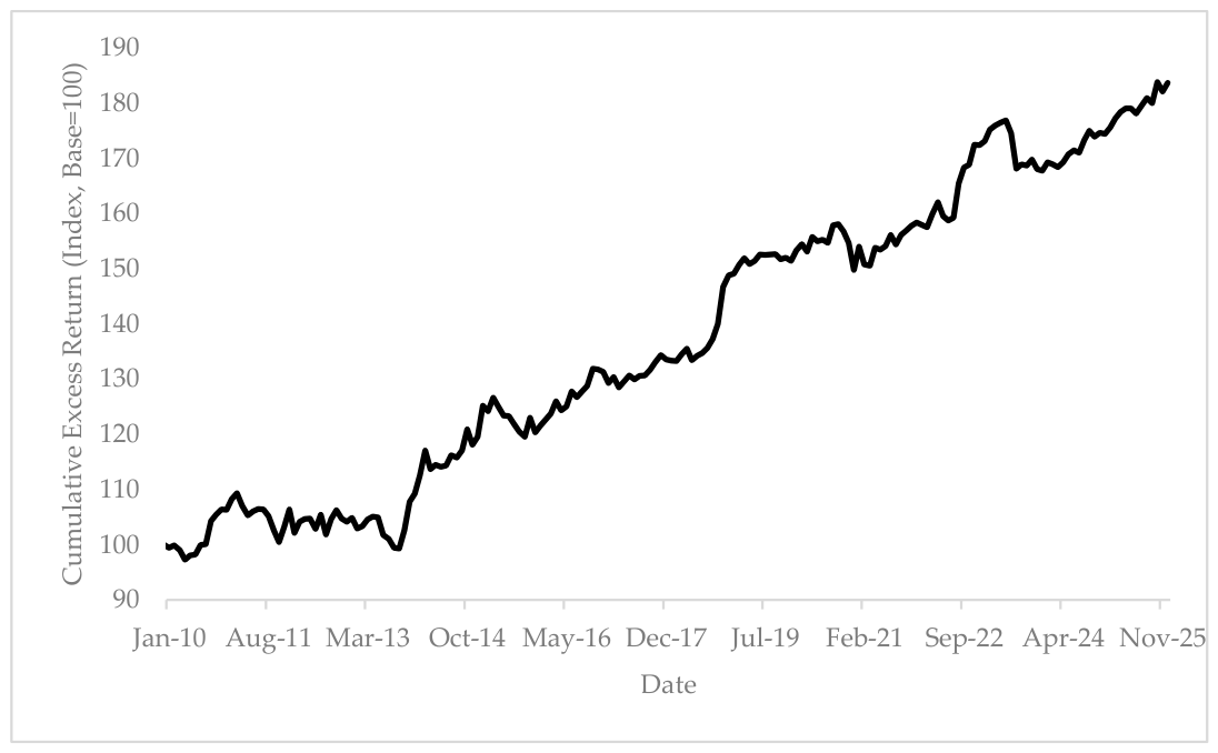
Figure 1 presents the cumulative long–short reversal excess returns over the sample period with the initial value set to 100. Overall, the cumulative excess return series exhibits a positive long-run trend, although the gains are not evenly distributed over time. This analysis complements the rolling-window evaluation by visualizing the gradual accumulation of short-term reversal profitability over extended horizons, which appears more consistent with the stronger results obtained under the 10-year rolling-window specification than under the 5-year horizon.

3.5. State-Dependent Performance and Factor Drawdowns

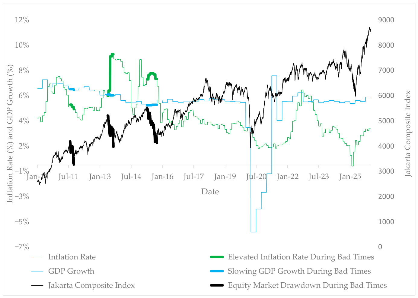
Figure 2 visualizes the evolution of macro-financial conditions and factor drawdowns, enabling an assessment of whether adverse environments coincide with declines in factor performance. Several marked episodes of stress are clearly identified. These periods are characterized by the joint occurrence of elevated inflation, slowing economic activity, and substantial stock market drawdowns, namely August–October 2011, May–August 2013, and April–September 2015. These periods are highlighted with thicker lines to distinguish them from the others. As defined in the methodology, they are classified as bad times, as all three conditions are satisfied simultaneously.

To assess the robustness of the bad-times classification, the models are re-estimated using alternative criteria, including a less stringent 15% stock market drawdown threshold and a definition of elevated inflation as inflation exceeding its sample median. The results remain broadly unchanged, as the identified bad-times episodes continue to largely coincide with those obtained under the baseline specification. This suggests that the classification is not overly sensitive to the specific thresholds adopted.

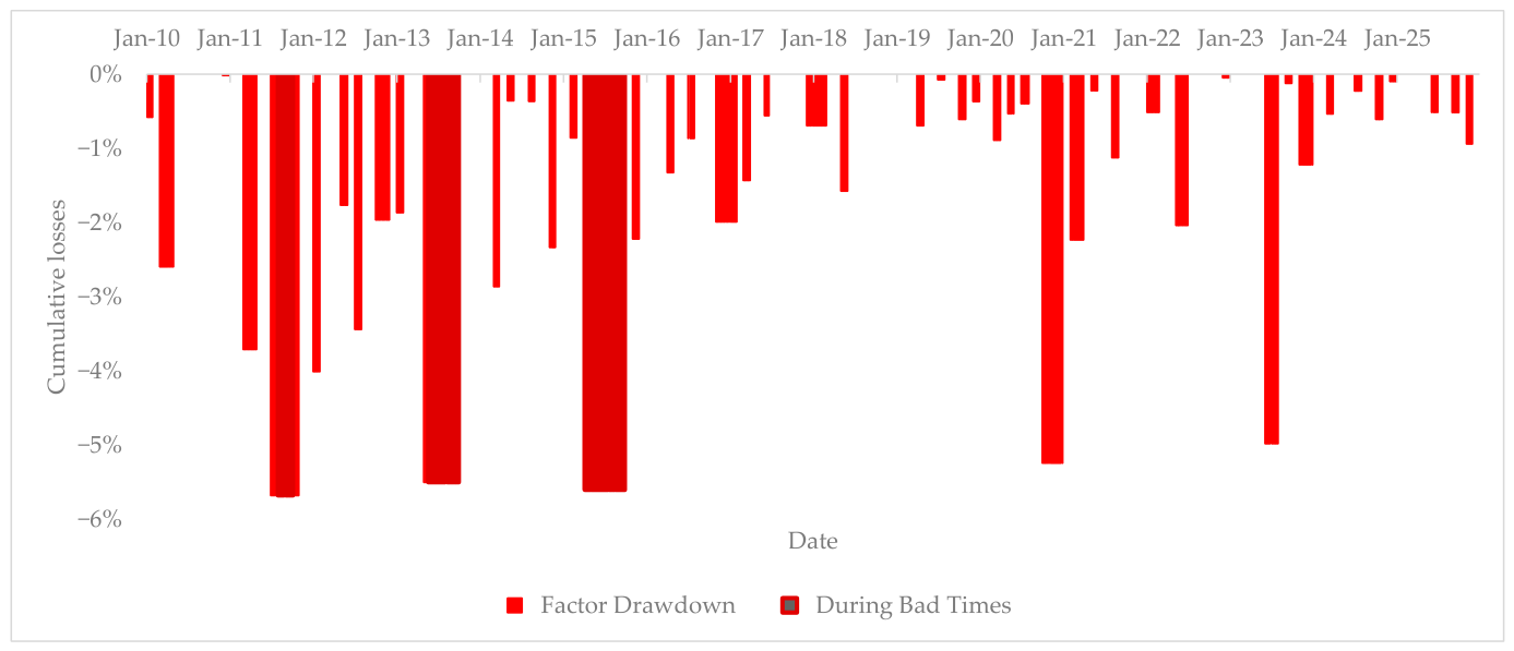
Figure 3 presents the timing and magnitude of factor drawdowns. Five major drawdown episodes are observed during the sample period, each associated with cumulative losses exceeding 5%. Three of these episodes occur during bad times (darker bars). While not all severe drawdowns coincide with bad times, the portfolio experiences performance deterioration during every bad-times episode, with losses generally becoming more pronounced.

To evaluate this relationship more formally, the next section presents regression-based evidence within a two-state framework. To assess whether the observed differences in factor performance across market conditions are statistically meaningful, the analysis employs a regression-based mean-difference test using Equation (7).

Table 8. Bad Times and Factor Portfolio Performance.

Coefficient	Estimate
Constant (t-stat)	0.43% (3.94) ***
Bad times dummy (t-stat)	−1.76% (−3.86) ***

Note: The dependent variable is the factor portfolio’s excess return. t-statistics are reported in parentheses. All figures rounded to two decimal places. Statistical significance is denoted by *** p < 0.01.

reports the estimation results.

The estimated constant of 0.43% indicates an average excess return of 0.43% per month during non–bad times (i.e., when the bad-times dummy equals zero), corresponding to approximately 5.15% annualized. The coefficient on the bad-times dummy (equal to 1 during bad times) is −1.76%, indicating that factor performance is, on average, 1.76 percentage points lower per month during bad times than during non–bad times. Consistent with the model specification, these estimates imply that the average monthly excess return during bad times is −1.33% (i.e., 0.43–1.76%), corresponding to approximately −15.92% annualized. Both coefficients are statistically significant at the 1% level, indicating a statistically significant difference in factor performance between bad and non–bad times, with an economically meaningful magnitude.

To further evaluate whether the documented bad-times effect persists after controlling for duration exposure,

Table 9. Bad Times and Duration-Neutral Factor Portfolio Performance.

Coefficient	Estimate
Constant (t-stat)	0.04% (3.36) ***
Bad times dummy (t-stat)	−0.08% (−1.97) **

Note: The dependent variable is the factor portfolio’s duration-adjusted excess return. t-statistics are reported in parentheses. All figures rounded to two decimal places. Statistical significance is denoted by *** p < 0.01, ** p < 0.05.

reports the regression results using the performance of the duration-neutral factor portfolio as the dependent variable. The estimated constant of 0.04% indicates positive average duration-adjusted excess returns during non–bad times, while the bad-times dummy coefficient of −0.08% indicates lower factor performance during bad times. Both coefficients remain statistically significant.

3.6. The Impact of Transaction Costs on Factor Performance

The practical viability of the reversal strategy is evaluated by incorporating the potential impact of transaction costs on net performance.

Table 10. Loser Portfolio Performance Before and After Transaction Costs.

Statistics	Before	After	Benchmark
Gross return	10.84%	10.84%	9.33%
Risk-free rate	5.64%	5.64%	5.64%
Breakeven transaction costs		1.50%
Net excess return	5.20%	3.70%	3.70%
Standard deviation of the net excess return	8.76%	8.76%	8.46%
Sharpe ratio	0.59	0.42	0.44
Net outperformance	1.50%	0.00%
Alpha (t-stat)	1.48% (2.67) ***	0.08% (0.14)

Note: All returns, costs, and volatilities are computed monthly, reported as sample averages, and annualized. Breakeven transaction costs are deducted only in the after-cost scenario. Net outperformance is the difference between a portfolio’s and a benchmark’s excess returns. Alpha (annualized) is estimated from regressions on benchmark excess returns, with Newey–West-adjusted t-statistics reported in parentheses. Statistical significance is denoted by *** p < 0.01.

shows portfolio performance before and after accounting for breakeven transaction costs—the point at which net outperformance over the benchmark drops to zero. This breakeven measure serves as an upper bound on trading cost for the strategy to remain benchmark-competitive, rather than representing an estimate of actual market costs. The simulation finds a breakeven cost of 0.125% per round-trip, or about 1.5% annually. When this cost is included, the loser portfolio no longer outperforms the benchmark.

4. Discussion

Understanding the performance of short-term reversal strategies in the Indonesian government bond market begins with examining the term structure of bond returns. Table 1 shows that average excess returns increase with maturity, accompanied by higher volatility. This pattern is consistent with the upward-sloping yield curve documented by Affandi et al. (2020) and aligns with liquidity preference theory, which posits that investors require additional compensation for holding longer-term bonds due to greater uncertainty surrounding interest rates and inflation (Fabozzi 2021).

The analysis then turns to the short-term reversal strategy. The reversal signals are computed for each bond, and bonds are sorted into portfolios based on signal rankings to examine cross-sectional return patterns. As reported in Table 2, the monotonic trend in the point estimates of average excess returns across bonds ranked from best to worst past performers has potential economic implications. Importantly, these return differences are not accompanied by proportionate increases in volatility as standard deviations remain broadly similar across signal groups. Consequently, the point estimate of the Sharpe ratios increases with signal strength, indicating improved risk-adjusted performance.

To assess whether these findings are driven by differences in interest rate exposure, the analysis examines the average duration across signal groups. The similarity in duration, together with the absence of statistically significant differences based on the Friedman test, suggests that the results are not driven by maturity effects, as bond rankings are broadly distributed along the yield curve.

As a robustness check, the analysis is repeated using duration-adjusted signals and excess returns. The results reported in Table 4 reinforce this conclusion. After adjusting both signals and returns for duration, the direction and ranking of returns across signal groups remain largely unchanged, indicating that the documented reversal effect cannot be fully attributed to maturity-related exposures.

At the portfolio level, the return patterns and contrasting alphas between the winner and loser portfolios suggest asymmetry in short-term reversal dynamics. Duration differences between the benchmark and both portfolios are also statistically insignificant. Furthermore, the factor portfolio exhibits lower volatility than the traditional long-only benchmark, consistent with reduced directional market exposure. The factor portfolio also generates a positive and statistically significant alpha, indicating performance beyond that captured by benchmark market movements during the sample period.

Although the return differential between the loser and winner portfolios is not statistically significant, applying the weighting scheme of Asness et al. (2013) consistently enhances performance. By assigning greater weights to bonds with more extreme signals, return differentials increase and become statistically significant, yielding significant factor returns. These findings suggest that signal-based weighting improves the extraction of factor premia. Overall, the evidence supports Hypothesis 1 (H1). The portfolio-level robustness checks using duration adjustment yield results that are broadly consistent with the baseline findings.

The temporal stability of the strategy is then evaluated using a rolling-window approach. Table 7 shows that performance becomes more stable over longer investment horizons. Higher success ratios in 10-year windows indicate long-term persistence, whereas lower ratios in 5-year windows reflect greater short-term variability. This pattern is consistent with Blitz (2011), who shows that factor premia are more robust over longer horizons but more volatile in the short run. These results support Hypothesis 2 (H2) and provide evidence of temporal persistence. However, this stability appears to be horizon-dependent, as the strategy’s success rate declines to approximately 61% over a five-year window, suggesting that shorter-horizon performance is more exposed to cyclical fluctuations and temporal instability.

Further analysis reveals that factor performance varies across macro-financial conditions. The three identified bad-time episodes occur during major global stress events—the European debt crisis (July–November 2011), the taper tantrum (May–September 2013), and the China slowdown (May–September 2015)—as documented by Harikrishnan et al. (2023). Notably, several of the most severe factor portfolio drawdowns occur during these episodes, indicating a systematic association between poor factor performance and adverse macro-financial conditions.

One possible mechanism relates to exchange-rate dynamics. Harikrishnan et al. (2023) documented that these episodes are associated with pronounced currency depreciation in emerging markets. This mechanism is particularly relevant in Indonesia, where foreign investors held approximately 14% to 40% of government bonds during the sample period. During periods of exchange rate volatility, foreign investors—who often evaluate returns in foreign-currency terms (IMF 2021)—may reduce their holdings, leading to capital outflows, downward pressure on bond prices, and upward pressure on yields. This interpretation aligns with the findings of Kurniasih and Restika (2015), who showed that exchange rates and foreign ownership jointly have a statistically significant impact on Indonesian government bond yields. The IMF (2021) also notes that Indonesia is more sensitive to capital outflows than many other emerging markets, reflecting its substantial foreign investor base and relatively high exchange rate volatility.

Regression results further confirm the state-dependent nature of factor performance. The strategy performs well under normal conditions but weakens during adverse periods. This pattern is consistent with a risk-based interpretation of factor premia (Ang 2014), whereby higher long-run returns compensate investors for bearing losses in bad times. These findings support Hypothesis 3 (H3).

From a broader asset-pricing perspective, these findings highlight the importance of evaluating factor premiums across different market states rather than relying solely on average returns. Consistent with Ang (2014) and Gormsen and Greenwood (2017), the evidence suggests that the economic relevance of a factor depends not only on its long-run profitability but also on its behavior during adverse conditions. In this context, the findings support the view that the reversal premium in the Indonesian government bond market compensates for risks that become particularly relevant under adverse market conditions.

To understand why the long–short strategy underperforms during bad times, this analysis examines how the portfolio’s risk composition evolves over these periods. As shown in the preceding analysis, bonds are broadly distributed across maturities, with no statistically significant differences in rankings across tenors.

Further analysis reveals a state-dependent shift in duration exposure between the loser and winner portfolios during bad times. Importantly, bad times in this study are defined by macro-financial conditions (e.g., inflation and economic growth) rather than by the direction of bond prices. During these periods, changes in yields create an asymmetric payoff structure.

Specifically, during the bond price declines of May–August 2013 and April–September 2015, loser portfolio durations increase to 9.7 and 8.6, respectively, while winner portfolio durations fall to 6.3 and 4.9. Consequently, losses on the long leg exceed gains on the short leg. In contrast, when bond prices rise (August–October 2011), this pattern reverses: the duration of loser portfolios declines to 5.9, whereas winner portfolios become more duration-intensive at 9.1. As a result, losses on the short leg outweigh gains on the long leg. Taken together, these findings suggest that variation in the relative duration of exposure of the long and short legs may contribute to the factor’s underperformance during some bad-time episodes.

To assess whether duration exposure fully accounts for the bad-times effect, the analysis is repeated using duration-adjusted signals and returns. The duration-adjusted results reported in Table 9 show that the long–short reversal strategy continues to perform significantly worse during bad times even after controlling for duration exposure. This persistence suggests that differences in duration alone cannot fully explain the factor’s vulnerability. Instead, the evidence points to broader state-dependent risks associated with adverse macro-financial conditions.

Market microstructure issues may also contribute to short-term reversal dynamics in the bond market (Khang and King 2004; Chordia et al. 2017). Given that government bond markets typically operate through a dealer-based market structure, inventory-related explanations provide a plausible institutional background for the observed reversal dynamics. Nevertheless, the present study does not aim to directly test market microstructure mechanisms. Rather, its primary objective is to document the state-dependent risk characteristics of short-term reversal profitability across different market conditions. Because the study does not directly observe dealer inventories, transaction-level order flow, or liquidity-provision behavior, these explanations are interpreted as complementary mechanisms rather than conclusively identified causal channels. In addition, higher liquidity is typically associated with narrower bid–ask spreads and lower inventory-related risks for dealers (Madhavan 2000), which may attenuate—though not necessarily eliminate—the role of inventory-driven price adjustments.

Behavioral explanations also cannot be entirely excluded, particularly given the extensive evidence documented in equity markets. However, such effects may be less pronounced in government bond markets, where trading activity is dominated by institutional investors operating under stricter risk-management frameworks and more valuation-driven investment processes. Supporting this view, Luo et al. (2025) note that contrarian behavior is typically driven by individual investors who believe other market participants have overreacted to news. In contrast, institutional investors are more inclined to employ momentum strategies or trade in line with news trends. Given the institutional dominance in the government bond market, this divergence in trading behavior further implies that behavioral overreaction is unlikely to be the primary driver of the observed short-term reversal effect.

Finally, the strategy’s practical feasibility is evaluated through transaction cost analysis. Evidence from ADB (2016, 2017, 2018, 2019, 2021, 2022, 2023, 2024) indicates that bid–ask spreads for on-the-run Indonesian government bonds range from 0.033% (3.3 basis points) to 0.053% (5.3 basis points). Treating the bid–ask spread as a proxy for round-trip transaction costs (Su and Tokmakcioglu 2021), these estimates remain well below the breakeven round-trip transaction cost of 0.125% (12.5 basis points), indicating that the strategy remains economically feasible under realistic trading conditions faced by institutional investors. This result reinforces the strategy’s practical relevance, indicating that the documented factor premia are not only statistically significant but also economically implementable.

This study contributes to the asset pricing literature in three ways. First, it provides evidence that short-term reversal strategies generate economically meaningful returns in the Indonesian government bond market. Second, it shows that reversal profitability is highly state-dependent, weakening significantly during periods of macro-financial stress. Third, it provides evidence that the strategy remains economically feasible after incorporating realistic transaction cost assumptions and focusing on liquid benchmark government bonds. Taken together, these findings suggest that short-term reversal can provide economically meaningful returns and remains practically feasible in the Indonesian government bond market, although its profitability varies across market conditions.

5. Data and Methods

5.1. Data

This study uses monthly data on Indonesian local-currency government bonds (rupiah-denominated) from January 2010 to December 2025. The sample spans several major global and domestic episodes, including the European sovereign debt crisis, the Taper Tantrum, China’s economic slowdown, and the COVID-19 crisis, thereby ensuring substantial variation in market and liquidity conditions.

The analysis focuses on four de jure benchmark government bonds with maturities of 5, 10, 15, and 20 years, designated annually by the Ministry of Finance. The Ministry of Finance typically announces benchmark bond designations on its official website, either at the end of the preceding year or at the beginning of the corresponding benchmark year. Benchmark bond series may vary from year to year and may include series designated in previous years. Several benchmark series remain classified as benchmarks across multiple years because their remaining maturities continue to approximate the target benchmark tenor while maintaining high market liquidity. In addition, benchmark bonds may migrate across tenor categories over time. For example, bonds previously designated as 15-year benchmarks may subsequently serve as 10-year benchmarks as their remaining maturities decline while preserving their benchmark liquidity status. The list of de jure benchmark bond series is presented in

Table 11. List of de jure Benchmark Bonds.

Year	5-Year	10-Year	15-Year	20-Year
2010	FR0027	FR0031	FR0040	FR0052
2011	FR0055	FR0053	FR0056	FR0054
2012	FR0060	FR0061	FR0059	FR0058
2013	FR0066	FR0063	FR0064	FR0065
2014	FR0069	FR0070	FR0071	FR0068
2015	FR0069	FR0070	FR0071	FR0068
2016	FR0053	FR0056	FR0073	FR0072
2017	FR0061	FR0059	FR0074	FR0072
2018	FR0063	FR0064	FR0065	FR0075
2019	FR0077	FR0078	FR0068	FR0079
2020	FR0081	FR0082	FR0080	FR0083
2021	FR0086	FR0087	FR0088	FR0083
2022	FR0090	FR0091	FR0093	FR0092
2023	FR0095	FR0096	FR0098	FR0097
2024	FR0101	FR0100	FR0098	FR0097
2025	FR0104	FR0103	FR0106	FR0107

.

These securities are identified as the most liquid instruments in the Indonesian market (Remolona and Yetman 2022). Evidence from the Annual Bond Market Liquidity Survey (ADB 2016, 2017, 2018, 2019, 2021, 2022, 2023, 2024) shows that on-the-run benchmarks exhibit narrower bid–ask spreads and larger transaction sizes than off-the-run bonds. Focusing on these liquid benchmarks ensures that the estimated factor signals and returns are based on securities that are realistically tradable and support monthly portfolio rebalancing. These securities account for about 15% of total local-currency government debt and constitute the core segment for institutional investors.

Information on coupon rates and maturities is obtained from the Ministry of Finance, while bond prices, the Jakarta Composite Index, and macroeconomic indicators—including year-on-year inflation, quarterly GDP growth, and local currency rate—are sourced from Bloomberg. Data screening reveals no outliers that materially affect the estimation results.

5.2. Empirical Framework

The methodological framework comprises four sequential stages. These are evaluating factor performance, assessing time persistence, providing a risk-based explanation, and estimating breakeven transaction costs. The following section elaborates on each stage.

5.2.1. Measuring Bond Returns and Excess Returns

To evaluate the profitability of our short-term reversal strategy, we first compute the individual monthly returns for each bond. The monthly return represents the percentage gain or loss from holding a bond for exactly one month, assuming the bond is purchased at the beginning of the month (using the previous month’s closing price) and sold at the end of the month (using the current month-end closing price). Following the methodology outlined by Teplova et al. (2020), we exclude coupon reinvestment from our calculation due to the short one-month holding period.

Consequently, the monthly return captures changes in the clean price, accrued interest, and any coupon payments actually received during that specific month. The raw monthly return is calculated using the following equation:

$$R_t^{\left[M\right]}={\displaystyle \frac{\left(P_t^{\left[M\right]}+{AI}_t^{\left[M\right]}+C_t^{\left[M\right]}\right)-\left(P_{t-1}^{\left[M\right]}+{AI}_{t-1}^{\left[M\right]}\right)}{\left(P_{t-1}^{\left[M\right]}+{AI}_{t-1}^{\left[M\right]}\right)}}$$

(1)

where $R_t^{\left[M\right]}$ represents the monthly return of the bond $\left[M\right]$ in month t, $P_t^{\left[M\right]}$ and $P_{t-1}^{\left[M\right]}$ correspond to the clean prices at the end of months t and t − 1, respectively, ${AI}_t^{\left[M\right]}$ and ${AI}_{t-1}^{\left[M\right]}$ indicate the accrued interest at the end of months t and t − 1, respectively, and $C_t^{\left[M\right]}$ denotes the coupon payment received between months t − 1 and t.

Once the raw monthly returns are determined, we calculate excess returns to isolate the risk premium earned by the bonds relative to a risk-free investment. The monthly excess return is computed by subtracting the prevailing risk-free rate from the bond’s raw monthly return:

$$E{R}_t^{\left[M\right]}=R_t^{\left[M\right]}-{\displaystyle \frac{R_t^f}{12}}$$

(2)

where ${ER}_t^{\left[M\right]}$ denotes the excess return of the bond $\left[M\right]$ in month t, $R_t^{\left[M\right]}$ represents the monthly bond return, and $R_t^f$ is the risk-free rate, proxied by the Bank Indonesia (BI) policy rate prevailing in month (t). The annual BI rate is divided by 12 to obtain a monthly simple risk-free return, ensuring consistency with the monthly bond return measure.

5.2.2. Constructing the Factor Portfolio

Following standard empirical practice in the short-term reversal literature (see Jegadeesh 1990), this study employs a rank-based approach to construct short-term reversal portfolios. At the end of each month t, each bond’s excess return for month t is calculated. The short-term reversal signal is defined as the negative of the excess return realized in month t (Maeso et al. 2019), such that bonds with lower contemporaneous returns receive stronger reversal signals. Signals are computed using realized returns over month t and are used to form portfolios at the beginning of month t + 1, whose returns are subsequently realized over month t + 1. This ensures that portfolio formation is based solely on information available at the end of the formation period.

Based on these estimated signals, the four bonds in the sample are ranked from B1 (lowest signal, corresponding to the best past performance) to B4 (highest signal, corresponding to the worst past performance). Two equally weighted long-only portfolios are formed at the beginning of month t + 1: Portfolio P1 (winner portfolio), comprising B1 and B2, and Portfolio P2 (loser portfolio), comprising B3 and B4. To capture cross-sectional return differentials, a long–short factor portfolio (hereafter referred to as the factor portfolio) is constructed at each rebalancing date by taking long positions in high-signal (loser) bonds (B3 and B4) and short positions in low-signal (winner) bonds (B1 and B2). Portfolio weights for the factor portfolio are assigned following the rank-based weighting scheme of Asness et al. (2013):

$$w_t^{\left[M\right]}=z_t\left[rank\left(S_t^{\left[M\right]}\right)-{\displaystyle \frac{\left(N_t+1\right)}{2}}\right]$$

(3)

where $w_t^{\left[M\right]}$ denotes the weight of the bond $\left[M\right]$ applied during month t + 1, $S_t^{\left[M\right]}$ represents the short-term reversal signal, $N_t$ is the number of bonds in the cross-section, and $z_t$ is a scaling factor that ensures that the sum of the long and short weights equals +1 and −1, respectively. Because the weights sum to zero across all bonds, the factor portfolio is dollar neutral. With $N=4$, the resulting weights are 0.75 for B4, 0.25 for B3, −0.25 for B2, and −0.75 for B1, assigning larger exposures to bonds with stronger signals.

All portfolios are evaluated using excess returns realized over month t + 1 and are rebalanced monthly at the beginning of each month based on signals computed at the end of the previous month. A benchmark portfolio representing the aggregate market is constructed as an equally weighted portfolio of all bonds and is held constant within each month, with rebalancing occurring only when the benchmark bond is replaced. This benchmark serves as the reference portfolio for estimating alphas of the winner, loser, and factor portfolios. Within this framework, Hypothesis 1 (H1) tests whether the short-term reversal factor generates positive and statistically significant excess returns.

5.2.3. Duration Adjustment as a Robustness Check

To ensure that the short-term reversal profitability is not solely driven by differences in duration exposure across bonds, this study implements a duration-adjusted reversal specification as a robustness check. The motivation follows the approach commonly used in bond carry strategies, as in Koijen et al. (2018), who argue that longer-maturity bonds tend to exhibit higher return volatility due to their greater sensitivity to interest-rate movements. Because the reversal signals are constructed from excess returns, which are inherently influenced by duration exposure, extending this adjustment to the reversal framework places bonds across maturities on a more comparable interest-rate-risk basis.

Specifically, the duration adjustment is implemented by dividing both the raw reversal signal and each bond’s excess return by its respective duration prior to portfolio formation. Following the approach employed by Koijen et al. (2018), the duration-adjusted short-term reversal signal, $\mathit{Adj} S_{t+1}^{\left[M\right]}$, and the duration-adjusted excess return, $\mathit{Adj} E{R}_t^{\left[M\right]}$, are defined as follows:

$$\mathit{Adj} S_{t+1}^{\left[M\right]}={\displaystyle \frac{{-ER}_t^{\left[M\right]}}{D_t^{\left[M\right]}}}$$

(4)

$$\mathit{Adj} E{R}_t^{\left[M\right]}={\displaystyle \frac{E{R}_t^{\left[M\right]}}{D_t^{\left[M\right]}}}$$

(5)

where $\mathit{Adj} S_{t+1}^{\left[M\right]}$ denotes the duration-adjusted reversal signal for the bond $\left[M\right]$ used for portfolio formation in month t + 1, and $\mathit{Adj} E{R}_t^{\left[M\right]}$ denotes the duration-adjusted excess return of the bond M in month t. $E{R}_t^{\left[M\right]}$ denotes the excess return of the bond $\left[M\right]$ in month t, while $D_t^{\left[M\right]}$ denotes the duration of the bond $\left[M\right]$ in month t. Duration is calculated using standard fixed-income conventions.

This scaling effectively assigns relatively smaller portfolio weights to longer-duration bonds and larger weights to shorter-duration bonds, thereby making interest-rate risk exposures more comparable across bonds. Both bond-level sorting and portfolio weighting are subsequently performed using the duration-adjusted reversal signal. Aside from this initial duration adjustment, the construction procedures for the winner, loser, and benchmark portfolios remain identical to those described in the previous section.

To maintain consistency with the duration-neutral portfolio construction commonly applied in bond factor strategies, the weighting scheme follows Martens et al. (2019) and is defined as follows:

$$Adj w_t^{\left[M\right]}=z_t\left[rank\left(Adj S_t^{\left[M\right]}\right)-{\displaystyle \frac{\left(N_t+1\right)}{2}}\right]$$

(6)

where $Adj w_t^{\left[M\right]}$ represents the portfolio weight assigned to the bond $M$ in month t based on the duration-adjusted short-term reversal signal. Consistent with Martens et al. (2019), the resulting long–short factor portfolio is constructed to be duration-neutral, with total duration exposure normalized to one year on both the long and short legs.

5.2.4. Evaluating Time Persistence

To assess the temporal stability of the factor portfolio’s performance, this study adopts a rolling-window approach, following Baltussen et al. (2022), updating it monthly over the full sample period. A 10-year rolling window serves as the baseline evaluation horizon. Within each window, factor performance is deemed successful if the factor portfolio generates a positive, statistically significant excess return.

To evaluate the sensitivity of persistence to the choice of evaluation horizon, the analysis is extended to a shorter, 5-year rolling window. Comparing results across these two horizons allows for an assessment of whether the stability of factor performance depends on the length of the evaluation window. This rolling-window framework provides a structured basis for evaluating Hypothesis 2 (H2), which concerns the persistence of factor performance over time.

As an additional robustness check, the study evaluates cumulative long–short portfolio excess returns following Coche et al. (2018). Specifically, cumulative excess returns are constructed by sequentially compounding the monthly excess returns generated by the reversal portfolio over the full sample period. The cumulative excess return analysis complements the rolling-window evaluation by providing a visual illustration of the long-horizon evolution of the reversal strategy’s profitability.

5.2.5. Risk-Based Explanation

The risk analysis in this study uses the two-state framework proposed by Gormsen and Greenwood (2017) to examine whether the factor portfolio’s performance is influenced by bad times. However, the empirical operationalization of bad times proposed by Gormsen and Greenwood (2017) requires several adjustments when applied to emerging markets such as Indonesia. Several local constraints need to be considered, including the rarity of technical recessions, the lack of housing market data, and the low frequency of unemployment statistics.

This study identifies three empirically feasible indicators of bad times in the Indonesian context: severe stock market drawdowns, slowing economic growth, and elevated inflation. These proxies are selected based on both their theoretical relevance and data availability. As demonstrated by Poterba (2000), sharp stock market declines reduce household wealth through a negative wealth effect. In addition, Rumbia et al. (2020) show that household spending significantly influences short-run economic growth, making economic slowdown a relevant proxy for deteriorating aggregate consumption conditions. Bachmann et al. (2015) further find that perceptions of high inflation are negatively associated with households’ willingness to spend on durable goods. Together, these variables are intended to capture periods of macro-financial stress in emerging markets such as Indonesia. The exact variables, thresholds, and classification rules are described as follows.

• Severe Stock Market Drawdowns

Severe stock market drawdowns are used as the primary indicator of financial distress (Gormsen and Greenwood 2017). A market drawdown is defined as the period between a local peak and the subsequent trough in the Jakarta Composite Index. Drawdowns are identified using daily data to mitigate end-of-month bias. All months between the identified peak and trough are classified as financially distressed, including the months at the peak and the trough. Short-lived recoveries within an ongoing decline do not alter the classification unless the drawdown is fully reversed, consistent with Gormsen and Greenwood (2017). To focus on economically meaningful distress, only severe drawdowns are considered, defined as drawdowns exceeding 20% from a previous peak, following Dabrowski (2022). Periods that do not meet this threshold are therefore not classified as financially distressed.

• Economic Slowdown

Because the NBER-style business cycle indicators are unavailable for Indonesia, and technical recessions—defined as two consecutive quarters of negative real GDP growth—are relatively rare during the sample period, this study adopts the concept of slowing economic conditions rather than formal recession episodes. This approach is broadly consistent with the bad-times perspective emphasized by Ang (2014). Specifically, economic conditions are classified as slowing when real GDP growth falls below the rate recorded in the corresponding period of the previous year. Because GDP data are available at quarterly frequency, the classification is applied to all months within the corresponding quarter. For example, if GDP growth in the second quarter is lower than in the same quarter of the previous year, all months within that quarter (April, May, and June) are classified as periods of economic slowdown.

• Elevated Inflation

Inflation is categorized as elevated when the inflation rate exceeds its sample average, consistent with Baltussen et al. (2022).

Furthermore, a period is designated as a bad-time episode only when all three conditions are simultaneously satisfied: (i) high inflation, (ii) slowing economic activity, and (iii) a market drawdown exceeding 20%. This joint-state definition follows Gormsen and Greenwood (2017) and captures both the economic and financial dimensions of adverse conditions.

While this strict definition may exclude some episodes that would qualify as bad times under more lenient criteria, it improves classification precision and strengthens the economic interpretation of the results. As such, the analysis focuses on periods that represent the most challenging environments for investors, providing a conservative and robust test of factor performance across states.

In addition, following Martens et al. (2019), this study evaluates factor drawdowns to identify both the timing and severity of performance declines. Their severity is measured by the absolute drawdown, which captures the cumulative loss sustained over consecutive negative-return periods (Schulmerich et al. 2015). This approach enables an assessment of whether bad times coincide with periods of declining strategy performance.

Having defined bad times, the analysis adopts a two-state framework following Baltussen et al. (2022) to distinguish between good and bad states. The following parsimonious regression is estimated to examine whether factor performance differs across these states:

$$R_t^F=\alpha +{\beta }_1{D}_t^{Bad times}+{\epsilon }_t$$

(7)

where $R_t^F$ denotes the excess return of the factor portfolio in the month $t$, and $D_t^{Bad times}$ equals one during bad times and zero otherwise. The coefficient ${\beta }_1$ captures the difference in performance between bad and good times. A negative, statistically significant estimate of ${\beta }_1$ indicates that the strategy performs worse during bad times, consistent with a risk-based interpretation (Ang 2014). This step corresponds to testing Hypothesis 3 (H3), which posits that the short-term reversal factor weakens under adverse conditions.

In emerging market economies (EMEs), including Indonesia, capital flows, financial conditions, and business cycles are often closely interconnected and tend to deteriorate simultaneously during periods of market stress (Juhro et al. 2024). Accordingly, the bad-times condition is intended to capture the joint influence of these macro-financial conditions, consistent with the bad-times perspective emphasized by Ang (2014) and the two-state framework discussed by Gormsen and Greenwood (2017). In addition, the state-dependent framework provides a more parsimonious way to capture the joint effects of macro-financial stress while reducing potential multicollinearity concerns that arise from including multiple highly correlated macroeconomic variables.

The objective is not to model return dynamics or establish causal relationships, but rather to provide a clear and interpretable diagnostic of whether factor performance systematically differs across macro-financial states, and to situate episodes of factor drawdowns within their broader economic context.

5.2.6. Assessing Practical Feasibility

Practical feasibility is evaluated by examining whether the strategy continues to deliver positive net outperformance after accounting for transaction costs. Performance is assessed relative to a passive benchmark, following Martens et al. (2019), where net outperformance is defined as the difference between the loser portfolio’s net excess return and the benchmark’s net excess return. To quantify cost tolerance, breakeven transaction costs are estimated—following Baltussen et al. (2021)—by incrementally increasing transaction costs until the net outperformance falls to zero. This breakeven threshold represents the maximum level of transaction costs at which the strategy remains competitive relative to the benchmark.

To assess practical implementability, the estimated breakeven threshold is compared with observed bid–ask spreads, which serve as a proxy for transaction costs, based on data reported in the Asia Bond Monitor published by the Asian Development Bank (ADB) for the Indonesian government bond market. The bid–ask spread, defined as the difference between the best bid and ask prices at a given point in time, captures explicit transaction costs and approximates the cost of executing a round-trip trade, consisting of consecutive buy-and-sell (or sell-and-buy) transactions of equal size (Su and Tokmakcioglu 2021). The comparison between the breakeven threshold and the bid–ask spread, therefore, offers a practical gauge of implementability.

The strategy is considered feasible when the breakeven threshold exceeds the prevailing bid-ask spread, indicating that net outperformance can be sustained under realistic trading conditions. While factor premia are identified using long–short portfolios, practical feasibility is evaluated using a long-only implementation—specifically, the loser portfolio—to reflect institutional constraints. Accordingly, the breakeven approach establishes an upper bound on transaction costs under realistic implementation.

6. Conclusions

This study provides supportive evidence that short-term reversal is a robust and economically meaningful characteristic of the benchmark segment of the Indonesian government bond market, with its performance exhibiting greater persistence over longer evaluation horizons. While short-term reversal has been documented in equity and corporate bond markets, evidence in government bond markets—particularly in emerging economies—remains limited. This study helps fill this gap by providing new evidence from the Indonesian government bond market.

The point estimates suggest a systematic tendency whereby bonds with weaker past performance are associated with higher subsequent excess returns. At the portfolio level, this effect translates into economically meaningful and statistically significant excess returns, particularly when signal-based weighting schemes are applied. Importantly, the results do not appear to be driven by conventional risk exposures such as duration. Further analysis using rolling-window estimation shows that this pattern persists across most subperiods, particularly over longer horizons, suggesting that the effect is not episodic but rather reflects a horizon-dependent regularity.

The evidence indicates that short-term reversal profitability exhibits state-dependent risk characteristics, with performance weakening during adverse economic and financial conditions. Although inventory-related mechanisms remain plausible in dealer-based bond markets, the study does not seek to directly identify market microstructure channels; rather, it documents the conditional nature of reversal profitability. From a practical perspective, transaction cost analysis provides supporting evidence of feasibility. Estimated breakeven transaction costs exceed observed bid–ask spreads, suggesting that the strategy is likely to remain economically feasible under realistic trading conditions, although bid–ask spreads represent only a partial proxy for total transaction costs.

In summary, this study extends the evidence on short-term reversal in government bond markets by integrating return predictability, state-dependent risk, and practical implementability within an emerging market setting. The findings contribute to a deeper understanding of factor behavior in fixed-income markets and highlight the importance of macro-financial conditions in shaping factor returns.

Nevertheless, several limitations should be acknowledged. First, as the study focuses on a single country, the generalizability of the findings to other markets remains uncertain. Future research may therefore extend the analysis to other emerging and developed government bond markets to evaluate whether similar reversal dynamics persist across different institutional and macroeconomic environments. At the same time, the single-country setting also offers analytical advantages. Previous cross-country studies, such as Zaremba and Czapkiewicz (2017) and Zaremba et al. (2019), have generally reported weaker or less consistent evidence of short-term reversal effects, possibly due to the use of pooled data from countries with heterogeneous market characteristics. In contrast, this study examines cross-maturity dynamics within a single and internally consistent domestic yield curve, thereby providing more granular evidence of reversal behavior in the Indonesian government bond market.

Second, the use of only four benchmark government bonds has important implications for interpreting the findings. By focusing on the most liquid segment of the Indonesian government bond market, the analysis is less affected by liquidity-related distortions and remains closely aligned with the investment universe of institutional investors, thereby enhancing the practical relevance and implementability of the results. However, the relatively small cross-sectional sample may reduce cross-sectional variation and limit the statistical power of portfolio-sorting exercises. In addition, the results may be more sensitive to tenor-specific dynamics and idiosyncratic price movements of individual bonds than studies employing broader bond universes. Consequently, the findings should be interpreted primarily as evidence from the liquid benchmark segment of the Indonesian government bond market and may not fully generalize to less-liquid government securities or other emerging bond markets. Accordingly, the sample selection represents a trade-off between practical relevance and cross-sectional breadth. Future research may address this limitation by incorporating broader bond universes, including off-the-run government and corporate bonds, to assess the robustness of the reversal effect across varying levels of liquidity and market segmentation.

Third, the findings are consistent with a state-dependent risk interpretation of reversal returns. However, this interpretation should be regarded as preliminary rather than definitive, as the present analysis does not directly identify the underlying causal mechanisms and cannot fully rule out alternative explanations. Although reversal performance deteriorates during bad times, the evidence does not establish that state-dependent risk fully explains the observed return patterns. Future research could further investigate the economic channels underlying reversal returns, including the roles of market microstructure and order flow. It may also explore whether machine-learning approaches provide additional insights into the dynamics of sovereign bond reversal strategies. In addition, cross-country analyses would help assess the extent to which these findings generalize beyond the Indonesian government bond market.

Overall, the results highlight the relevance of factor-based strategies in emerging bond markets and provide a foundation for future research on return predictability in fixed-income markets.

References

1. Affandi, Yoga, Berry Harahap, Pakasa Bary, and Fenty P. Suryani. 2020. Natural yield curve: The case of Indonesia. Contemporary Economics 14: 182–200. [Google Scholar] [CrossRef]
2. Aghassi, Michele, Cliff Asness, Charles Fattouche, and Tobias J. Moskowitz. 2023. Fact, fiction, and factor investing. Journal of Portfolio Management 49: 57–94. [Google Scholar] [CrossRef]
3. Ang, Andrew. 2014. Asset Management: A Systematic Approach to Factor Investing. New York: Oxford University Press. [Google Scholar] [CrossRef]
4. Arnott, Rob, Vitali Kalesnik, and Lillian Wu. 2023. Mitigating the hidden risks of factor investing. Journal of Portfolio Management 49: 111–24. [Google Scholar] [CrossRef]
5. Asian Development Bank. 2016. Asia Bond Monitor: November 2016. Manila: Asian Development Bank. Available online: https://www.adb.org/sites/default/files/publication/213241/abm-nov-2016.pdf (accessed on 11 June 2026).
6. Asian Development Bank. 2017. Asia Bond Monitor: November 2017. Manila: Asian Development Bank. [Google Scholar] [CrossRef]
7. Asian Development Bank. 2018. Asia Bond Monitor: November 2018. Manila: Asian Development Bank. [Google Scholar] [CrossRef]
8. Asian Development Bank. 2019. Asia Bond Monitor: November 2019. Manila: Asian Development Bank. [Google Scholar] [CrossRef]
9. Asian Development Bank. 2021. Asia Bond Monitor: March 2021. Manila: Asian Development Bank. [Google Scholar] [CrossRef]
10. Asian Development Bank. 2022. Asia Bond Monitor: March 2022. Manila: Asian Development Bank. [Google Scholar] [CrossRef]
11. Asian Development Bank. 2023. Asia Bond Monitor: March 2023. Manila: Asian Development Bank. [Google Scholar] [CrossRef]
12. Asian Development Bank. 2024. Asia Bond Monitor: March 2024. Manila: Asian Development Bank. [Google Scholar] [CrossRef]
13. Asian Development Bank. 2025a. Asia Bond Monitor: June 2025. Manila: Asian Development Bank. [Google Scholar] [CrossRef]
14. Asian Development Bank. 2025b. AsianBondsOnline. Available online: https://asianbondsonline.adb.org/data-portal/ (accessed on 10 September 2025).
15. Asness, Cliff, Tobias J. Moskowitz, and Lasse Heje Pedersen. 2013. Value and momentum everywhere. Journal of Finance 68: 929–85. [Google Scholar] [CrossRef]
16. Avramov, Doron, Tarun Chordia, and Amit Goyal. 2006. The impact of trades on daily volatility. Review of Financial Studies 19: 1241–77. [Google Scholar] [CrossRef]
17. Bachmann, Rüdiger, Tim O Berg, and Eric R. Sims. 2015. Inflation expectations and readiness to spend: Cross-sectional evidence. American Economic Journal: Economic Policy 7: 1–35. [Google Scholar] [CrossRef]
18. Baltussen, Guido, Martin Martens, and Olaf Penninga. 2021. Predicting bond returns: 70 years of international evidence. Financial Analysts Journal 77: 133–55. [Google Scholar] [CrossRef]
19. Baltussen, Guido, Martin Martens, and Olaf Penninga. 2022. Factor investing in government bond markets: Deep sample evidence. Journal of Portfolio Management 48: 209–25. [Google Scholar] [CrossRef]
20. Blitz, David. 2011. Strategic allocation to premiums in the equity market. In SSRN Electronic Journal. Rochester: Social Science Research Network. [Google Scholar] [CrossRef]
21. Breeden, Douglas T. 1979. An intertemporal asset pricing model with stochastic consumption and investment opportunities. Journal of Financial Economics 7: 265–96. [Google Scholar] [CrossRef]
22. Butt, Hilal Anwar, Kenneth Högholm, and Mohsin Sadaqat. 2021. Reversal returns and expected returns from liquidity provision: Evidence from emerging markets. Journal of Multinational Financial Management 59: 100664. [Google Scholar] [CrossRef]
23. Chernov, Mikhail, Drew Creal, and Peter Hördahl. 2023. Sovereign credit and exchange rate risks: Evidence from Asia-Pacific local currency bonds. Journal of International Economics 140: 103692. [Google Scholar] [CrossRef]
24. Chordia, Tarun, Amit Goyal, Yoshio Nozawa, Avanidhar Subrahmanyam, and Qing Tong. 2017. Are capital market anomalies common to equity and corporate bond markets? An empirical investigation. Journal of Financial and Quantitative Analysis 52: 1301–42. [Google Scholar] [CrossRef]
25. Coche, Joachim, Mark Knezevic, and Vahe Sahakyan. 2018. Carry on? In Advances in the Practice of Public Investment Management: Portfolio Modeling, Performance Attribution and Governance. Edited by Narayan Bulusu, Joachim Coche, Alejandro Reveiz, Francisco Rivadeneyra, Vahe Sahakyan and Ghislain Yanou. Cham: Palgrave Macmillan, pp. 131–59. [Google Scholar] [CrossRef]
26. Conrad, Jennifer, Mustafa N. Gultekin, and Gautam Kaul. 1997. Profitability of short-term contrarian strategies: Implications for market efficiency. Journal of Business and Economic Statistics 15: 379–86. [Google Scholar] [CrossRef]
27. Dabrowski, Piotr. 2022. Stock indices breakdown during the pandemic as the most dynamic bear market in history: Consequences for individual investors. Risks 10: 1. [Google Scholar] [CrossRef]
28. Dai, Wei, Mamdouh Medhat, Robert Novy-Marx, and Savina Rizova. 2023. Reversals and the Returns to Liquidity Provision (NBER Working Paper No. 30917). Cambridge: National Bureau of Economic Research. Available online: https://ssrn.com/abstract=4349550 (accessed on 11 June 2026).
29. Fabozzi, Frank J. 2021. Bond pricing, yield measures, and total return. In The Handbook of Fixed Income Securities, 9th ed. Edited by Frank J. Fabozzi. New York: McGraw-Hill, pp. 63–95. [Google Scholar]
30. Fong, Tom Pak Wing, and Shui Tang Wu. 2020. Predictability in government bond returns using technical trading rules: Do developed and emerging markets differ? North American Journal of Economics and Finance 61: 101105. [Google Scholar] [CrossRef]
31. Galariotis, Emilios C. 2014. Contrarian and momentum trading: A review of the literature. Review of Behavioral Finance 6: 63–82. [Google Scholar] [CrossRef]
32. Gormsen, Niels, and Robin Greenwood. 2017. Rainy Day Stocks (Working Paper No. 17-066). Boston: Harvard Business School. Available online: https://www.hbs.edu/faculty/Pages/item.aspx?num=52149 (accessed on 11 June 2026).
33. Hamdan, Rayyan, Fabien Pavlowsky, Thierry Roncalli, and Ban Zheng. 2016. A primer on alternative risk premia. In SSRN Electronic Journal. Rochester: Social Science Research Network. [Google Scholar] [CrossRef][Green Version]
34. Harikrishnan, Nira, Benjamin Silk, and Emre Yoldas. 2023. U.S. Interest Rates and Emerging Market Currencies: Taking Stock 10 Years After the Taper Tantrum. Washington: Board of Governors of the Federal Reserve System. [Google Scholar] [CrossRef]
35. Ilmanen, Antti, Ronin Israel, Tobias J. Moskowitz, Aswin K. Thapar, and Rachel Lee. 2021. How Do Factor Premia Vary Over Time? A Century of Evidence. Rochester: Social Science Research Network. Available online: https://ssrn.com/abstract=3400998 (accessed on 11 June 2026).
36. International Monetary Fund. 2021. Indonesia: Selected Issues. IMF Staff Country Report No. 2021/047. Washington: International Monetary Fund. [CrossRef]
37. Jegadeesh, Narasimhan. 1990. Evidence of predictable behavior of security returns. Journal of Finance 45: 881–98. [Google Scholar] [CrossRef]
38. Jegadeesh, Narasimhan, and Sheridan Titman. 1995. Overreaction, delayed reaction, and contrarian profits. Review of Financial Studies 8: 973–93. [Google Scholar] [CrossRef]
39. Juhro, Solikin M, Bernard Njindan, and Paresh Kumar Narayan. 2024. Capital flow dynamics and the synchronization of financial cycles and business cycles in emerging market economies. Journal of International Financial Markets, Institutions and Money 92: 101980. [Google Scholar] [CrossRef]
40. Kassimatis, Konstantinos, Spyros Spyrou, and Emilios Galariotis. 2008. Short-term patterns in government bond returns following market shocks: International evidence. International Review of Financial Analysis 17: 903–24. [Google Scholar] [CrossRef]
41. Khang, Kenneth, and Tao-Hsien Dolly King. 2004. Return reversals in the bond market: Evidence and causes. Journal of Banking and Finance 28: 569–93. [Google Scholar] [CrossRef]
42. Koijen, Ralph S. J., Tobias J. Moskowitz, Lasse Heje Pedersen, and Evert B. Vrugt. 2018. Carry. Journal of Financial Economics 127: 197–225. [Google Scholar] [CrossRef]
43. Kurniasih, Augustina, and Yulia Restika. 2015. The influence of macroeconomic indicators and foreign ownership on government bond yields: A case of Indonesia. Mediterranean Journal of Social Sciences 6: 34–42. [Google Scholar] [CrossRef]
44. Lo, Andrew W., and Craig MacKinlay. 1990. When are contrarian profits due to stock market overreaction? Review of Financial Studies 3: 175–205. [Google Scholar] [CrossRef]
45. Luo, Patrick, Enrichetta Ravina, Marco C. Sammon, and Luis M Viceira. 2025. Retail Investors’ Contrarian Behavior Around News, Attention, and the Momentum Effect (NBER Working Paper No. 34086). Cambridge, MA: National Bureau of Economic Research. Available online: http://www.nber.org/papers/w34086 (accessed on 11 June 2026).
46. Madhavan, Ananth. 2000. Market microstructure: A survey. Journal of Financial Markets 3: 205–58. [Google Scholar] [CrossRef]
47. Maeso, Jean Michel, Lionel Martellini, and Ricardo Rebonato. 2019. Factor Investing in Fixed-Income—Cross-Sectional and Time-Series Momentum in Government Bond Markets. Singapore: EDHEC-Risk Institute. Available online: https://www.edhec.edu/sites/default/files/ckeditor-inlines/Factor-Investing-in-Fixed-Income-Cross-Sectional-and-Times-Series-Momentum-in-Sovereign-Bond-Markets.pdf (accessed on 11 June 2026).
48. Martens, Martin, Paul Beekhuizen, Johan Duyvesteyn, and Casper Zomerdijk. 2019. Carry investing on the yield curve. Financial Analysts Journal 75: 51–63. [Google Scholar] [CrossRef]
49. Medhat, Mamdouh, and Maik Schmeling. 2022. Short-term momentum. Review of Financial Studies 35: 1480–526. [Google Scholar] [CrossRef]
50. Moskowitz, Tobias J., and Mark Grinblatt. 1999. Do industries explain momentum? Journal of Finance 54: 1249–90. [Google Scholar] [CrossRef]
51. Poterba, James M. 2000. Stock market wealth and consumption. Journal of Economic Perspectives 14: 99–118. [Google Scholar] [CrossRef]
52. Remolona, Eli, and Yetman James. 2022. De jure benchmark bonds. International Journal of Central Banking 18: 89–124. [Google Scholar] [CrossRef]
53. Rumbia, Wali Aya, Abd Azis Muthalib, Bakhtiar Abbas, Pasrun Adam, Heppi Millia, Laode Saidi, and Muh. Irfandi Azis. 2020. Crude oil prices, household spending and economic growth in the ASEAN-4 region: An analysis of nonlinear panel autoregressive distributed lag. International Journal of Energy Economics and Policy 10: 437–42. [Google Scholar] [CrossRef]
54. Schulmerich, Marcus, Yves-Michel Leporcher, and Ching-Hwa Eu. 2015. Applied Asset and Risk Management: A Guide to Modern Portfolio Management and Behavior-Driven Markets. Berlin/Heidelberg: Springer. [Google Scholar] [CrossRef]
55. Su, Emre, and Kaya Tokmakcioglu. 2021. A comparison of bid-ask spread proxies and determinants of bond bid-ask spread. Borsa Istanbul Review 21: 227–38. [Google Scholar] [CrossRef]
56. Subrahmanyam, Avanidhar. 2005. Distinguishing between rationales for short-horizon predictability of stock returns. Financial Review 40: 11–35. [Google Scholar] [CrossRef]
57. Teplova, Tamara, Tatiana V. Sokolova, and Qaiser Munir, eds. 2020. Which investment strategy is profitable in bond market? Reverse or momentum? What about risk? In Emerging Bond Markets: Shedding Light on Trends and Patterns. London: Routledge, pp. 290–304. [Google Scholar] [CrossRef]
58. Yen, Gili, and Cheng Few Lee. 2008. Efficient market hypothesis (EMH): Past, present and future. Review of Pacific Basin Financial Markets and Policies 11: 305–29. [Google Scholar] [CrossRef]
59. Zaremba, Adam, and Anna Czapkiewicz. 2017. The cross section of international government bond returns. Economic Modelling 66: 171–83. [Google Scholar] [CrossRef]
60. Zaremba, Adam, Huaigang Long, and Andreas Karathanasopoulos. 2019. Short-term momentum (almost) everywhere. Journal of International Financial Markets, Institutions and Money 63: 101140. [Google Scholar] [CrossRef]
Figure 1. Cumulative Excess Returns of the Factor Portfolio (2010–2025).
Risks 14 00137 g001
Figure 2. Market Drawdowns, Macroeconomic Conditions, and Bad-Times Episodes. Note: Bad times are defined at the monthly level as periods when three conditions occur simultaneously: (1) a stock market drawdown exceeding 20% from a previous peak, (2) inflation exceeding its sample average of 4%, and (3) real GDP growth below the rate recorded in the corresponding period of the previous year. Thickened line segments highlight observations corresponding to bad-times episodes. The stock market index is observed daily, while inflation and GDP are available at monthly and quarterly frequencies, respectively. For graphical comparability, each monthly (quarterly) observation is assigned to all days within the corresponding month (quarter), such that values remain constant within each period.
Risks 14 00137 g002
Figure 3. Factor Drawdowns and Bad-Times Episodes. Note: Drawdown episodes are identified from peak to trough, with drawdown magnitude measured as the cumulative loss sustained over consecutive negative-return periods. Darker bars indicate factor drawdowns that coincide with bad-times episodes defined in Figure 2.
Risks 14 00137 g003