The Impact of Climate Change on Banking System Stability in Southern Africa Development Communities (SADC)

Abstract

In today’s world, climate change has become a global predicament. The implications for financial sector activities have given rise to ample literature on the climate change and banking system stability nexus in developing economies. However, there still remain important knowledge gaps pertaining to areas such as the asymmetric impact of climate change on banking system relationships, threshold effects, and transmission channels. Therefore, this research investigated the impact of climate change on banking system stability in the Southern Africa Development Communities (SADC). The study employed a panel data estimation technique, analysing fixed and random effects to test these hypotheses in SADC. In doing so, it not only explored how climate-related risks affect banking stability but also assessed how economic, environmental, and institutional dynamics mediate this relationship. The findings contribute to informing regional policy on financial resilience and adaptive climate strategies within fragile banking environments.

1. Introduction

Climate change has emerged as one of the most pressing global challenges of our time. The effects of climate change go beyond ecological bounds and penetrate national, regional, and international socioeconomic structures. Climate change is a relevant banking risk factor emanating from banking services when they provide lending and financial products or services to firms located in areas more vulnerable to climate risk (Javadi and Masum 2021).

Climate change, broadly defined as long term alterations in temperature, precipitation patterns, and extreme weather events, has far reaching consequences for global economic systems, particularly financial institutions. In the context of banking, climate-related risks are typically classified into physical risks arising from climate-induced disasters such as floods, veld fires, heatwaves, and droughts, as well as transition risks which stem from the economic shifts associated with the move toward a low-carbon economy, like carbon pricing, CO₂ emissions, and policy indices.

These risks threaten the stability of banks by impairing asset values, increasing default probabilities, and disrupting credit and liquidity flows. In developing regions such as the Southern Africa Development Communities (SADC), where economies are highly vulnerable to environmental shocks and institutional capacities are often constrained, the financial implications of climate change are especially pronounced. The European Central Bank (2023) stated that the European Union (EU) made economic losses amounting to approximately five hundred and sixty (€560) billion euros between 1980 and 2021 due to disasters caused by climate change.

The African region, which incorporates the SADC, is highly vulnerable to negative climate change effects as the region depends on agriculture and mining, which are sensitive to physical climate change risks affecting lives, animals, and plants (UNEP FI 2023). Against this backdrop, disasters related to climate change like droughts, floods, tornadoes, hurricanes, and extreme heatwaves occur more frequently nowadays, raising physical and transition risks that affect the financial sector, causing instability (Beck 2023).

Battiston et al. (2021), Le et al. (2023), and Zhou and Ma (2025) showed that climate change risk has two possible transmission streams, namely physical and transition risk. The Bank of England (BoE) (2018) notes that banks have begun assessing the impact of climate change through physical risks such as floods, droughts, storms, heatwaves, and variations in precipitation, as well as transition risks, and are integrating these considerations into their business models.

In addition, the former Bank of England governor, Mark Carney, explains that climate change impacts financial stability via three main channels: physical risks, liability risks, and transition risks (Carney 2015). It is worth mentioning that physical risk relates to weather and climate-related events such as storms, heatwaves, and floods that destroy properties or impede trade, as well as insurance liabilities, and the value of financial assets. Further, liability risk mainly affects financial stability due to the potential consequences that might occur if people who have lost something or experienced harm because of climate change demand payment from those they believe to be at fault (ibid.).

Climate physical risks have been shown to result in losses from weather events linked to climate change, affecting physical assets, natural capital, and human lives (Monasterolo 2020). Transition risk emanates from financial and operational challenges that arise as economies shift toward low-carbon and more sustainable models. This includes changes in policy, technology, market preferences, and regulatory frameworks aimed at reducing greenhouse gas emissions. According to Le et al. (2023), such risks can significantly impact the value of carbon-intensive assets and the overall stability of financial institutions navigating this transition. Mueller and Sfrappini (2022) pointed out that due to climate change challenges and threats, the global community is now shifting towards a more sustainable and environmentally friendly productive system and economy.

The SADC is a regional community made up of sixteen (16) member states with different climate patterns and banking system operations. The 16 member states include Angola, Botswana, Comoros, Democratic Republic of Congo, Eswatini, Lesotho, Madagascar, Malawi, Mauritius, Mozambique, Namibia, Seychelles, South Africa, United Republic of Tanzania, Zambia, and Zimbabwe. According to Wamukonya and Rukato (2001), the ability of the Southern Africa region to adapt to climate change is its biggest problem. It is crucial to note that the effects of climate change are varied throughout Southern Africa, and that various economies may experience difficulties depending on their geographic location, climate zone, and socioeconomic status. Over the past few decades, temperatures in Southern Africa have increased, as evident in other parts of the world.

Despite the growing interest in climate change and banking system studies, economic and finance literature has paid limited attention to the Southern Africa Development Communities (SADCs). Some studies have examined the effects of climate change on sectors such as tourism (Amusan and Olutola 2017; Fitchett 2021; Sibitane 2022) and economic growth and development (Raubenheimer and Phiri 2023). Others have investigated how climate change has influenced asset prices and corporate policies after climate-related events have occurred or climate risks have materialised (Nie et al. 2023; Huynh et al. 2020).

Evidently, studies before us had modelled a climate change framework for financial stress-testing in Southern Africa—although the authors’ research focused only on South Africa, leaving out the other fifteen member states of SADC (Anvari et al. 2022; Wu et al. 2024). A 2023 report by the Africa Development Bank (AfDB) establishes that Southern Africa’s economic prospects are subdued yet abound with investment opportunities in climate change initiatives.

A rise in temperature has the potential to cause several environmental problems, such as changes in precipitation patterns, higher rates of evaporation, and heatwaves. It is documented that Southern Africa is vulnerable to extreme weather conditions, with the warming of the interior occurring at about twice the global average rate (Scholes and Engelbrecht 2021). In the context of the banking sector, Adu et al. (2024) highlight that financial institutions in Southern Africa are becoming increasingly aware of the far-reaching implications of climate change. This underscores the growing concern over extreme weather events and flooding, which are emerging as critical risk factors affecting the stability of banking operations and the value of financial assets.

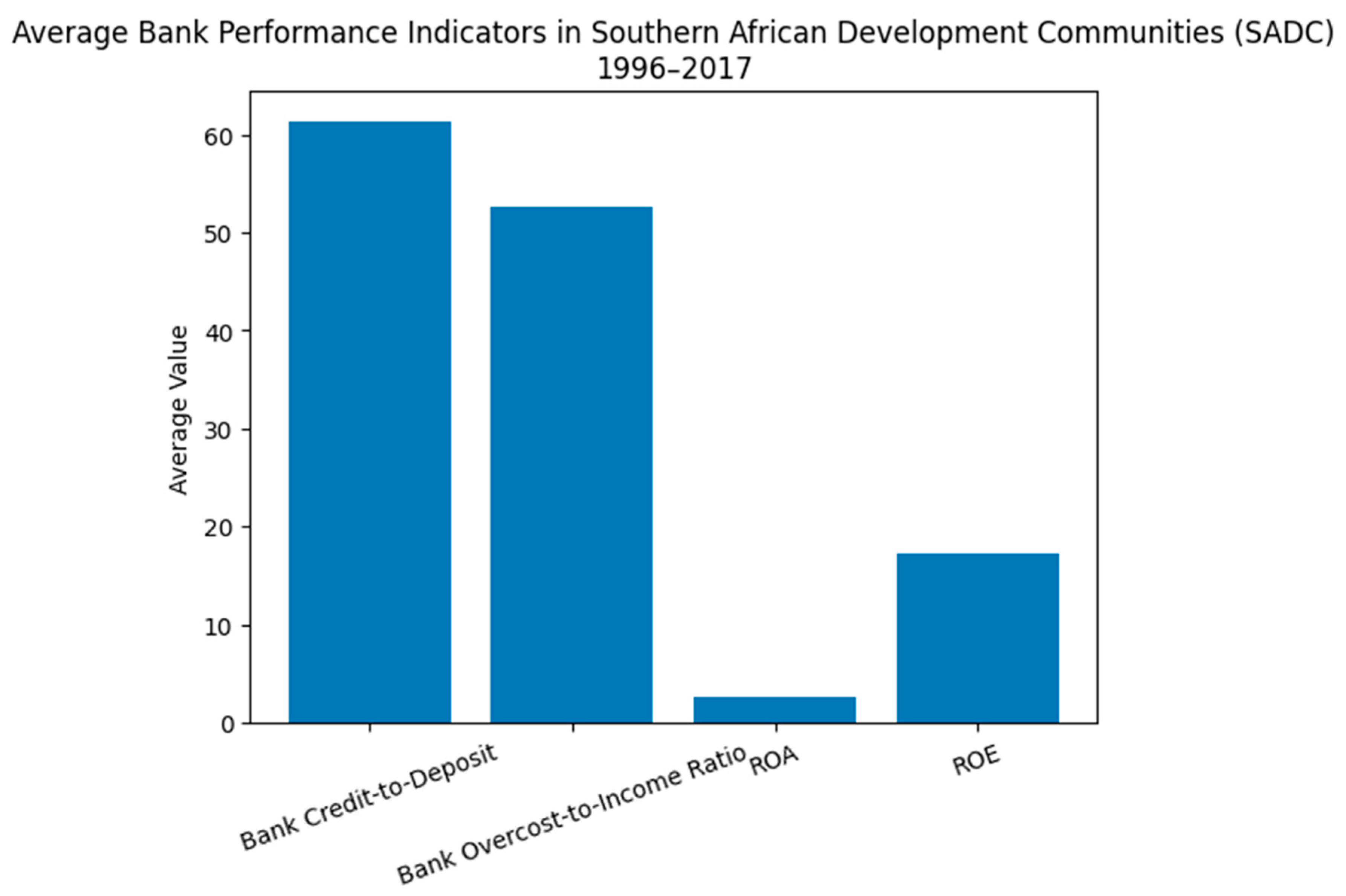
Climate change-related risks raise financial sector challenges and increase risks affecting banking operations as well as bank performance, efficiency, and profitability. On that note, we present a graphical illustration of selected banking sector performance indicators motivated by Mahawiya (2016) and Akande (2018) to analyse the banking sector performance in SADC.

From Figure 1, it is inferred that Southern Africa banking systems have seen significant performance in the selected bank-specific indicators. It is revealed that bank credit-to-deposit in the region is 61.30 percent, signifying good credit progression. In addition, the bank’s cost-to-income ratio was recorded at 52.67 percent. This indicates that banking sectors in the region are less efficient. The bank cost-to-income ratio is used to gauge efficiency; thus, the lower the bank cost-to-income ratio, the higher the efficiency, vice versa. For the profitability indicators, return on assets (ROA) and return on equity (ROE) in the region are 2.65 and 17.28, respectively. The reported profitability value implies that the banking sectors in the region are profitable and make judicious use of their resources.

Due to the nature of the banking sector performance in SADC and the region’s susceptibility to climate change, the issue calls for further investigation. To date, whether climate change is ruinous to banking system activities in the SADC is clearly missing in academic empirics. To close this gap, this research examines the relation between climate change and the stability of the banking systems in the SADC. The main research question guiding this study is: How does climate change impact the stability of the banking system within the SADC region? More specifically, it builds on existing studies (Amo-Bediako et al. 2023; Agbloyor et al. 2021; Do et al. 2023) to answer the following questions: Does climate change have a negative impact on banking system stability in SADC? Are there threshold effects in the interaction between climate change and banking system stability? What are the transmission channels through which climate change affects banking system stability?

This study specifically focuses on how climate change affects banking system stability in the SADC, addressing gaps in the literature by investigating asymmetric effects, threshold dynamics, and the mechanisms through which climate risks are transmitted into the banking sector. The study explicitly examines the relationship between climate change and banking system stability in the SADC region by focusing on measurable climate indicators such as average temperature anomalies, frequency of extreme weather events like droughts and floods, and carbon emissions as proxies for climate risk.

To address the research gap identified in the existing literature, this study builds on prior empirical and theoretical work on climate risk and financial stability by focusing specifically on the banking sector within the Southern African Development Community (SADC). While previous studies have examined climate change impacts on financial markets and individual economies, limited attention has been given to cross-country banking system performance in Southern Africa. Accordingly, this research investigates the relationship between climate change risk and banking system stability by examining how physical and transition risks influence key bank performance indicators across SADC member states. The significance of the study lies in its contribution to understanding climate-related financial vulnerabilities in emerging economies and providing evidence-based insights to support climate-sensitive banking regulation, risk management strategies, and sustainable financial development within the SADC region.

The study adopts a quantitative panel data approach using econometric modelling techniques to evaluate the effects of climate-related variables on indicators such as credit-to-deposit ratios, cost-to-income ratios, return on assets (ROA), and return on equity (ROE). By employing panel regression analysis and comparative regional data, the research seeks to provide empirical evidence on whether climate change risk weakens banking performance and financial stability. The findings are expected to contribute to policy debates by highlighting the need for climate-sensitive financial regulation and risk management strategies within emerging economies, particularly those highly exposed to environmental shocks.

Bank stability is assessed using key financial soundness indicators, including return on assets (ROA), non-performing loans (NPLs), and the Z-score, which collectively capture profitability, credit risk, and insolvency risk. The analysis covers a balanced panel of all SADC countries for the period from 1996 to 2017, using yearly data where available. The research questions are addressed through panel data econometric techniques, such as fixed and random effects, and threshold regression, to test for asymmetric effects and explore transmission mechanisms.

The main objective of this study is to empirically assess the impact of climate change on banking system stability in the Southern Africa Development Communities (SADC), by identifying the nature, extent, and channels through which climate-related risks influence key financial stability indicators across the region. The remainder of the paper is sectionalized as follows. Section 2 presents a brief literature review guiding the direction of this study. In Section 3, we describe the data. We present the methodology in Section 4. Section 5 discusses the empirical findings. Section 6 concludes the paper and provides policy recommendations.

2. Literature Review

Given the scale of the implications of climate change, scholars have begun presenting new ideas on the relationship between climate change and financial activities. The intersection between climate change and banking system stability has garnered increasing scholarly attention due to the complex ways in which environmental disruptions affect financial systems. Climate-related risks are broadly categorised into physical risks stemming from acute events such as floods, hurricanes, and wildfires, or chronic shifts like rising temperatures and sea levels, as well as transition risks, which arise from the policy, legal, technological, and market changes required for a low-carbon economy.

Both types of risks can undermine banking stability through several transmission channels, including loan defaults, asset revaluation, operational disruptions, increased insurance costs, and liquidity shortages. The effects are often magnified in emerging markets and developing countries (EM/DCs), where economies are highly exposed to climate-sensitive sectors like agriculture, and where financial systems may lack diversification, robust regulation, and adaptive capacity. Compared to advanced economies (AEs), financial institutions in EM/DCs are more vulnerable to these climate shocks due to limited fiscal buffers, institutional fragility, and high exposure concentrations.

Theoretical contributions have illustrated that both forms of climate risk influence the financial system through direct balance sheet effects and indirect macroeconomic channels. For example, asset devaluation due to chronic drought may deteriorate collateral values, while transition risk from abrupt carbon emission or pricing reforms may impair the viability of carbon-intensive investments (Amo-Bediako and Takawira 2025). Theoretical models also suggest that the climate–financial relationship may be non-linear, with moderate environmental stress sometimes fostering innovation or policy response, while extreme stress leads to systemic instability. Furthermore, asymmetry in the climate-bank stability nexus has been posited, where adverse shocks produce more severe consequences than favourable shifts, a dynamic particularly relevant in under-diversified financial systems.

Carbon pricing has emerged as a significant tool for managing climate-related financial risks and shaping the stability trajectory of banking systems. The introduction of carbon taxes and emissions trading systems leads to increased costs for carbon-intensive firms, which may translate into heightened credit risks for banks with high exposure to such sectors. As noted by Agbloyor et al. (2021), the relationship between carbon emissions and banking stability is evident globally, particularly where financial institutions fail to reallocate capital toward low-carbon ventures. Banks heavily invested in fossil-fuel-based sectors are more vulnerable to asset stranding and defaults, a concern amplified in emerging markets where carbon-intensive industries often dominate. Studies by Amo-Bediako et al. (2023) further affirm that climate shocks, magnified by inadequate adaptation strategies and inconsistent regulatory frameworks, compromise the resilience of Sub-Saharan banking systems. In this context, the stability of banks becomes contingent on their capacity to assess and incorporate carbon-related risks into credit scoring and portfolio diversification strategies.

On the other hand, carbon pricing can also catalyse opportunities for financial innovation and long-term sustainability. Adu et al. (2024) argue that when banks align their corporate governance with climate initiatives, carbon pricing serves not as a risk amplifier but as a strategic lever for sustainable profitability. Effective internal governance mechanisms enable banks to reorient capital flows toward green sectors, enhancing resilience and competitive advantage. In regions like Southern Africa, where institutions such as the South African Reserve Bank (SARB) have begun incorporating climate scenarios into stress testing (Anvari et al. 2022), the integration of carbon emission or pricing into financial models provides a buffer against future shocks. However, this transition is not without challenges. As Amusan and Olutola (2017) and Arndt et al. (2020) emphasise, the socio-political dynamics and regulatory inertia in developing regions can hinder the financial sector’s adaptive capacity. Thus, the relationship between carbon emissions or pricing and bank stability is dualistic, posing systemic risks for unprepared institutions, while fostering sustainability and resilience for forward-looking banks embedded in well-regulated environments.

Empirical studies provide evidence for these mechanisms. Masunda (2025) finds that climate risk significantly weakens financial sector stability in selected SADC countries, particularly through rising carbon emissions and non-performing loans that transmit climate shocks into banking vulnerabilities. The study further shows that integrating climate risk into prudential regulation and financial supervision is essential for strengthening resilience, as empirical results reveal a statistically significant negative long-run relationship between climate risk and financial stability. Do et al. (2023) examined the impact of acute physical risks, namely natural disasters, on United States (US) bank stability using data from 907 banks and the SHELDUS database. The study found a non-linear deterioration in bank resilience following events such as floods and heatwaves, supporting the theory that disaster-driven economic disruptions increase loan defaults and reduce customer deposits.

Le et al. (2023) offered a broader view by assessing the effects of both physical and transition risks across 6433 banks in 109 countries (2008–2019). Their analysis confirmed a negative relationship between climate risks and bank stability, highlighting the global scale of vulnerability. Wu et al. (2023), Amo-Bediako et al. (2023), and Meng et al. (2023) highlight that climate change brings negative consequences for the financial sector, and the impacts are profound and far-reaching. On the other hand, Liu et al. (2021) allude that uncertainty is a paramount feature of climate change, and it will be challenging to evaluate its implications on the global economy. In present times, climate change is increasingly recognised by monetary and financial regulators, yet empirical evidence on its implications for bank system stability is scant (Nie et al. 2023).

According to Javadi and Masum (2021), risks emanating from climate change are crucial to macroeconomic development, growth, and financial stability. In addition, the consequences of climate change are evident in financial system operations (ibid.). The Bank for International Settlements (BIS 2021) suggests that monetary authorities have begun to understand and quantify climate change impacts in the banking sector. Despite this clairvoyance, Do et al. (2023) explicate that the trend and intensity of extreme weather events have an enormous impact on banking system operations and performance.

Needless to say, banks play a pivotal role in the interplay between climate change and the general economy (Lamperti et al. 2021). Arndt et al. (2020) posit that climate change mitigation will enormously prove to be a crucial structural change. Interestingly, the Paris Agreement signed in 2016, has intensified the debate on the relationship between climate change and financial stability (Carney 2015). The Intergovernmental Panel for Climate Change (IPCC 2018) defines climate change as the change in the state of the climate that can be identified through changes in mean or the variations in its properties using statistical approaches.

Zhang et al. (2022) focused on transition risks in China using network analysis and discovered that the move toward a low-carbon economy has heightened systemic risk dependencies among financial institutions. This suggests that poorly coordinated climate policy shifts can generate new vulnerabilities. Liu et al. (2021) used NARDL and vector autoregression to analyse the asymmetric effect of chronic temperature changes on China’s financial stability. Their findings support the theory that climate impacts are non-linear and asymmetric, as both increases and decreases in temperature disrupt financial markets.

Pagnottoni et al. (2022) extended the literature to stock markets, finding that the financial response to natural hazard shocks (such as biological, climatological, geophysical, and meteorological disasters) varied depending on the event type and location. This spatial heterogeneity underscores how the intensity and geography of climate events influence financial outcomes. Wu et al. (2023) corroborated these findings by showing that temperature deviation—a measure of chronic physical risk—negatively affects China’s financial system. These studies affirm that environmental stress impairs borrower solvency, reduces investment confidence, and ultimately erodes banking system resilience.

Region-specific research adds nuance. Kimundi and Wambui (2023) analysed climate risk transmission in Kenya and found agriculture to be the main channel for physical risks, while manufacturing is emerging as a channel for transition risks. They further noted that sectors key to climate policy implementation—like energy, transport, construction, and agriculture—are increasingly interconnected with banking system health, suggesting that the structure of the economy significantly influences the propagation of climate risks.

Agbloyor et al. (2021) investigated the relationship between carbon emissions (as a proxy for transition risk) and bank stability across 122 countries from 2000 to 2013. The study revealed an inverted U-shaped trend: at lower levels, carbon emissions are associated with economic growth and stability, but beyond a threshold, increased carbon emissions correlate with declining financial resilience. This supports the theory of a non-linear climate–finance relationship, implying that the marginal impact of emissions and carbon pricing on banking stability intensifies beyond certain levels.

Despite these important contributions, several theoretical and empirical gaps persist. First, few studies examine how the structural characteristics of the financial and economic system—such as sectoral concentration, financial depth, and regulatory robustness—mediate the transmission of climate risks. Second, the asymmetric and non-linear effects of climate change on bank stability remain underexplored in the SADC, a region particularly vulnerable to climate variability and with structural financial fragility. Third, while some studies consider transition and physical risks jointly, there is a need to disentangle their differential effects and identify potential thresholds beyond which stability erodes rapidly.

This study addresses these gaps by focusing on both types of climate risk and their theoretical and empirical impacts on bank stability across the SADC region. It applies panel data estimation techniques to assess asymmetric and non-linear relationships, accounting for structural mediators such as sectoral exposure and institutional capacity. In doing so, the research contributes to both theoretical clarity and policy relevance in understanding climate-induced financial vulnerabilities in developing economies.

3. Data and Sources

Annual data from 1996 to 2017 for 16 SADC economies were utilised. The study focuses on the 16 SADC economies because they represent a geographically integrated regional bloc with comparable climate exposure and financial structures, while the 1996–2017 period is selected based on consistent data availability and reliability from international databases, ensuring balanced panel analysis and methodological robustness. Following the work of Amo-Bediako et al. (2023) and Amo-Bediako et al. (2024a, 2024b), we employed the Z-score as a banking system stability measure. In this paper, we follow the definition of Adusei (2015) in selecting the Z-score as a stability measure. Adusei (2015) defines stability as the number of standard deviations a bank’s assets (ROA) must drop for the bank to become insolvent. That notwithstanding, Takawira (2022) states that definitions pertaining to the stability of banks are cloudy, and there are no clear-cut adjustments for their measurement. Intrinsically, Agbloyor et al. (2021) argue that returns and capitalization are compared using the Z-score, and the higher the Z-score, the more banking sectors are stable (Agbloyor et al. 2021). We glean climate change variables such as temperature and precipitation data from the Climate Change Knowledge Portal. In addition, carbon emission data were taken from WDI.

The study includes bank concentration and bank efficiency as financial system control variables with data sourced from the Global Finance Database. We expect a positive outcome between bank concentration, bank efficiency, and banking system stability. The intuition is that bank concentration can reduce competition, which leads to a higher profit margin and increased stability. Further, bank concentration increases market power, which allows banks to better manage their risk and maintain stability. On the other hand, an increase in bank efficiency improves asset quality and capital adequacy, reduces operational costs, and increases risk management processes.

More so, the study adds macroeconomic variables like inflation and real GDP as part of the control variables. Intuitively, we expect a negative relationship between inflation and banking stability. The onus lies on the assertion that higher inflation rates reduce banking system stability. With real GDP and banking system stability, we expect a positive relationship between the two estimates. More importantly, inflation influences banking system stability through the monetary policy transmission mechanism. As such, higher interest rates may negatively affect lending activities. Further, inflation can impact banking system stability via the credit channel. Thus, higher interest rates can increase credit risk and negatively affect lending activities. Inflation can also impact banking system stability through the asset price channel. Thus, higher inflation rates can reduce asset values and increase the risk of default.

It is important to highlight that regulatory quality is included in the regression model as a proxy for governance measurement. We expect a positive relationship between regulatory quality and banking system stability on the background that high-quality regulation enhances risk management practices, improves capital requirements, enhances transparency and disclosure, as well as improves supervision and enforcement, which reduces the likelihood of instability. The data for the regulatory quality is taken from the World Governance Indicator platform. For the transmission channel, we include manufacturing value added (as a percentage of GDP) and agriculture value added (as a percentage of GDP) as a multiplicative interactive term. We expect either a positive or negative outcome from the transmission interaction of manufacturing value added, agriculture value added, and climate change on banking system stability.

Stylised notations/expected signs and source of the data to be employed in the study are presented in

Table 1. Stylised notations/expected signs and data sources.

Variable	Notation	Expected Sign	Source
Dependent Variable
Banking System Stability	STAB		Global Finance Development Database
Independent Variable(s)
Temperature	TEMPT	−	Climate Knowledge Portal
Precipitation	PPT	−	Climate Knowledge Portal
Carbon Emissions	CO2	−	Climate Knowledge Portal
Bank-Specific Variable(s)
Bank Concentration	BC	+	Global Finance Development Database
Bank Efficiency	BE	+	Global Finance Development Database
Macroeconomic Variable (s)
Inflation	INFL	−	WDI
Real Gross Domestic Product	RGDP	+	WDI
Transmission Channel
Manufacturing Value Added	MVA	±	WDI
Agriculture Value Added	AVA	±	WDI
Governance Variable
Regulatory Quality	RQ	+	WGI

Source: author’s construct, 2024.

.

4. Methodology

This section illustrates the methodology, econometric model data used, and their sources. It further shows the economic model and model specification applied in this study. The study utilised a quantitative approach, analysing annual data from the SADC region.

4.1. Economic Model

The dependent variable is banking system stability in a particular SADC country at a particular time. Bank system stability is measured using indicators like Z-score, non-performing loan ratios, or capital adequacy ratios. This study makes use of the Z-score as a proxy of bank system stability, and the calculation is shown in Appendix A. The main independent variables include explanatory variables that capture climate change risks, bank-specific variables, and control variables. The economic model under study and analysed through panel regression analysis -fixed effects (FE) and random effects (RE), is shown below:

$$\begin{array}{c}{BankSystemStability}_{it}\hfill \\ ={\beta }_0+{PhysicalRisk}_{it}{\beta }_1+{TransitionRisk}_{it}{\beta }_2+{ClimateRiskThreshold}_{it}{\beta }_3\\ +{BankConcentration}_{it}{\beta }_4+{BankEfficiency}_{it}{\beta }_5+{Inflation}_{it}{\beta }_6\\ +{RealGrossDomesticProduct}_{it}{\beta }_7+{RegulatoryQuality}_{it}{\beta }_8+{\mu }_i+{\lambda }_t+{\epsilon }_{it}\end{array}$$

(1)

where

-

${PhysicalRisk}_{it}$: A quantitative proxy for physical climate risks, temperature deviations, and precipitation.

-

${TransitionRisk}_{it}$: Variable representing transition risks, which includes carbon emissions.

-

${ClimateRiskThreshold}_{it}$: Variable capturing interaction terms between climate variables.

-

Control variables include real GDP, inflation, bank concentration and efficiency, and regulatory quality. Transmission channels were applied using value added from manufacturing and agriculture.

-

${\mu }_i$: Country-specific fixed effects.

-

${\lambda }_t$: Time fixed effects.

-

${\epsilon }_{it}$: Error term.

4.2. Model Specification

The study capitalises on a panel data framework to investigate the nexus between climate change and banking system stability. The empirical methodologies of this study focus on examining the relationship between climate change and banking system stability in the SADC region. Second, the threshold effects of climate change and banking system stability in SADC. Lastly, the transmission channels through which climate change impacts banking system stability. Herein, we follow the work of Amo-Bediako et al. (2024a, 2024b) to construct a 3-step econometric model for this topical debate.

Climate change denotes a set of climate change variables, which include average temperature, changes in precipitation, and reduction of carbon dioxide (CO₂) emission termed decarbonization, as adopted from Pointner and Ritzberger-Grünwald (2019) and Liu et al. (2021). Again, CONT symbolises control variables such as gleaned from financial system factors, such as bank concentration and bank efficiency, as well as macroeconomic variables like inflation and real gross domestic product. In addition, governance indicators such as regulatory quality were included in the model specification. Importantly, the model will be individually specified as follows:

$$Sta{b}_{it}={(TEMPT,BC,BE,INFL,RGDP,RQ)}_{it}$$

(2)

$$Sta{b}_{it}={(PPT,BC,BE,INFL,RGDP,RQ)}_{it}$$

(3)

$$Sta{b}_{it}={(C{O}_2,BC,BE,INFL,RGDP,RQ)}_{it}$$

(4)

We expand models (2)–(4) and econometrically specify them as follows:

$$Sta{b}_{it}={\delta }_{it}+{\varphi }_{1}TEMP{T}_{it}+{\varphi }_{2}B{C}_{it}+{\varphi }_{3}B{E}_{it}+{\varphi }_{4}INF{L}_{it}+{\varphi }_{5}RGD{P}_{it}+{\varphi }_{6}R{Q}_{it}+{\mu }_{it}$$

(5)

$$Sta{b}_{it}={\phi }_{it}+{\theta }_{1}PP{T}_{it}+{\theta }_{2}B{C}_{it}+{\theta }_{3}B{E}_{it}+{\theta }_{4}INF{L}_{it}+{\theta }_{5}RGD{P}_{it}+{\theta }_{6}R{Q}_{it}+{\mu }_{it}$$

(6)

$$Sta{b}_{it}={\sigma }_{it}+{\psi }_{1}C{O}_{2it}+{\psi }_{2}B{C}_{it}+{\psi }_{3}B{E}_{it}+{\psi }_{4}INF{L}_{it}+{\psi }_{5}RGD{P}_{it}+{\psi }_{6}R{Q}_{it}+{\mu }_{it}$$

(7)

where $\delta ,\phi ,\sigma$ indicate intercepts for models (5)–(7). Also, ${\varphi }_1,{\varphi }_2,{\varphi }_3,{\varphi }_4,{\varphi }_5,{\varphi }_6$ are coefficients for model (5). ${\theta }_1,{\theta }_2,{\theta }_3,{\theta }_4,{\theta }_5,{\theta }_6$ are the coefficients of model (6). Coefficients of model (7) are shown as ${\psi }_1,{\psi }_2,{\psi }_3,{\psi }_4,{\psi }_5,{\psi }_6$. $i$ and $t$ represent the cross-section units and time periods. Model (5)–(7) will be transformed with the introduction of a natural logarithm. Therefore, the above models will be specified as follow:

$$Sta{b}_{it}={\delta }_{it}+{\varphi }_1\ln TEMP{T}_{it}+{\varphi }_2\ln B{C}_{it}+{\varphi }_3\ln B{E}_{it}+{\varphi }_4\ln INF{L}_{it}+{\varphi }_5\ln RGD{P}_{it}+{\varphi }_6\ln R{Q}_{it}+{\mu }_{it}$$

(8)

$$Sta{b}_{it}={\phi }_{it}+{\theta }_1\ln PP{T}_{it}+{\theta }_2\ln B{C}_{it}+{\theta }_3\ln B{E}_{it}+{\theta }_4\ln INF{L}_{it}+{\theta }_5\ln RGD{P}_{it}+{\theta }_6\ln R{Q}_{it}+{\mu }_{it}$$

(9)

$$Sta{b}_{it}={\sigma }_{it}+{\psi }_{1}C{O}_{2it}+{\psi }_2\ln B{C}_{it}+{\psi }_3\ln B{E}_{it}+{\psi }_4\ln INF{L}_{it}+{\psi }_5\ln RGD{P}_{it}+{\psi }_6\ln R{Q}_{it}+{\mu }_{it}$$

(10)

Again, the research employs a threshold regression model to simultaneously choose the tipping point at which climate change impacts banking system stability in SADC. Motivated by this, the study utilises the Hansen (1999) threshold regression for the estimation technique. Essentially, respective threshold models of climate change clusters are specified below.

$$\ln Sta{b}_{it}={\beta }_0+{\varpi }_{1}TEMP{T}_{it}I(TEMP{T}_{it}\le \gamma )+{\varpi }_{2}TEMP{T}_{it}I(TEMP{T}_{it}\ge \gamma )+{\varpi }_3{Z}_{it}+{\kappa }_{it}$$

(11)

$$\ln Sta{b}_{it}={\beta }_0+{\varpi }_{1}PP{T}_{it}I(PP{T}_{it}\le \gamma )+{\varpi }_{2}PP{T}_{it}I(PP{T}_{it}\ge \gamma )+{\varpi }_3{Z}_{it}+{\kappa }_{it}$$

(12)

$$\ln Sta{b}_{it}={\beta }_0+{\varpi }_{1}C{O}_{2it}I(C{O}_{2it}\le \gamma )+{\varpi }_{2}C{O}_{2it}I(C{O}_{2it}\ge \gamma )+{\varpi }_3{Z}_{it}+{\kappa }_{it}$$

(13)

where $Stab$, $TEMPT$, $PPT$ and $C{O}_2$ are earlier defined. $I(.)$ is an indicator function and $\gamma$ is the threshold for specified climate change variables. The regimes (low/high) are denoted by two regression slopes of coefficients ${\varpi }_1$ and ${\varpi }_2$.

It is worth mentioning that the paper again examines the transmission streams through which climate change impacts banking system stability. On that account, we introduce a multiplicative interaction term of climate change. In particular, we specify the transmission equation where the indirect effect is measured as $\omega$. We proxy manufacturing value added (MVA) as a percentage of GDP and agriculture value added (AVA) as a percentage of GDP as the interactive terms. Further, we adopt the wavelet coherence technique to analyse the transmission channels. The wavelet analytical approach was applied to analyse macroeconomic transmission pathways through which climate change affects banking system stability. The wavelet method helps to identify the correlations and impacts of variables. In light of this, Aawaar (2017) contends that wavelets merge time and frequency dimensions and use phase difference approaches to capture structural changes in data.

5. Empirical Findings and Discussion

This section illustrates the results of this study and provides an analysis of the findings.

5.1. Summary Statistics

Table 2. Summary Statistics of variables.

	Minimum	Maximum	Mean	Std, Deviation	Variance	Skewness	Kurtosis
Stab	0.000	96.680	9.166	8.421	70.906	4.516	0.130
Tempt	−0.530	2.800	0.547	0.481	0.231	1.120	0.130
CO2	0.016	104.860	5.004	15.411	237.491	4.262	0.130
PPT	0.000	2753.920	986.442	491.954	242,018.777	0.640	0.130
BC	0.000	100.000	59.280	36.578	1337.963	−0.722	0.130
BE	0.000	112.245	50.280	22.898	524.306	−0.809	0.130
INFL	−9.616	4145.106	37.950	227.055	51,554.152	17.031	0.130
RGDP	351,136,579.649	458,201,514,136.976	27,341,607,897.243	69,206,581,561.042	4,789,550,931,365,100,000,000.000	4.227	0.130
RQ	−2.202	1.127	−0.423	0.704	0.496	−0.118	0.130

Source: author’s construct, 2024.

shows the summary statistics of the variables utilised in the study. The summary statistics reveal significant variation across the dataset’s key variables, indicating a diverse economic and climatic landscape among the observations. The descriptive statistics provide valuable insights into the distributional characteristics and variability of the panel data variables used in the analysis. Banking system stability (Stab) displays a mean of approximately 9.17 with a high standard deviation of 8.42, indicating substantial dispersion around the mean. The variable is highly positively skewed (skewness = 4.52) and exhibits extreme kurtosis (36.95), suggesting the presence of severe outliers and a heavy-tailed distribution. Similar patterns are observed for CO₂ emissions, inflation (INFL), and real GDP (RGDP). CO₂ emissions, with a mean of 5.00 and a standard deviation of 15.41, are heavily right-skewed (skewness = 4.26) with a kurtosis of 18.58, indicating infrequent but extremely high emission levels in certain observations. Inflation displays an even more pronounced departure from normality, with a staggering skewness of 17.03 and a kurtosis of 307.39. This suggests extremely volatile inflation episodes across the sample. RGDP shows a similar trend with a very large spread (standard deviation of ~69 billion) and highly non-normal distribution, likely due to large disparities in economic size across countries or regions. The mean value of standard deviation asserts that banks in SADC are generally stable with some fluctuations.

In contrast, variables such as temperature (Tempt), bank efficiency (BE), and regulatory quality (RQ) demonstrate more symmetric and less extreme distributions. Temperature has a mean of 0.55 with a low standard deviation of 0.48, showing modest variation and only mild positive skewness. Bank efficiency, with a mean of 50.28 and a standard deviation of 22.90, shows a slightly left-skewed but approximately normal distribution (kurtosis = 0.51), making it relatively well-suited for regression analysis. Regulatory quality is nearly symmetric (skewness = −0.12) and also exhibits limited kurtosis (−0.42), indicating a well-behaved distribution. Precipitation (PPT) and bank concentration (BC) fall somewhere in between, with moderate variability and manageable distributional characteristics. Overall, these statistics highlight that while some variables are suitable for direct inclusion in regression models, others—particularly those with extreme skewness and kurtosis like INFL, CO₂, and RGDP—may require transformation (e.g., logarithmic), outlier management, or robust estimation techniques to ensure valid inference in subsequent econometric analyses.

Temperature (Tempt) and precipitation (PPT), representing climate variables, show moderate and high variation, respectively, highlighting environmental heterogeneity. Carbon emissions (CO₂), bank capitalization (BC), and bank efficiency (BE) show moderate dispersion, reflecting differences in financial access, capital adequacy, and operational performance across banks. It is important to highlight that the variations in the climate change variables permit the establishment of important policies in line with the assessment of thresholds. This depicts that banks in SADC are not operating at optimal levels, suggesting waste and inefficiency in their operations.

On inflation, the results suggest that the SADC experiences moderate inflation that is beneficial for economic growth, as it can stimulate spending and investment. Real GDP (RGDP) shows substantial differences in economic size, while regulatory quality (RQ) varies moderately, pointing to uneven institutional strength. This shows that SADC economies have been growing at a moderate pace, with a minimum growth rate signalling relative economic shock resilience. Poor regulation affects the investment climate; thus, foreign investment, as investors prefer countries with a stable and predictable regulatory environment. Together, these statistics underscore the need for appropriate econometric models that can capture the effects of climate and macroeconomic conditions on banking stability.

5.2. Test Statistics

5.2.1. Cross-Sectional Dependence Test 1

We employ the cross-sectional dependence test of Breusch and Pagan (1980), thus the LM test to detect significant correlation between the residuals of different cross-sectional units. The LM test was chosen because the cross-section is lower than the time period. Again, the cross-sectional dependence test is applied to avoid biased and inconsistent estimates, improve the model specification, and increase the robustness of the outcome, as well as enhance policy recommendations. We present the results of Breusch and Pagan’s (1980) LM test for the individual variables in

Table 3. Cross-sectional dependence test results (variables).

Test Statistics
Variable	LM Test
lnStab	784.564 (0.000) ***
lnTempt	210.000 (0.000) ***
lnPPT	292.002 (0.000) ***
lnCO2	784.564 (0.000) ***
lnBC	738.483 (0.000) ***
lnBE	315 (0.000) ***
lnINFL	399.580 (0.000) ***
lnRGDP	1290.447 (0.000) ***

Source: author’s construct, 2024. *** denotes statistical significance at the 1% level (p < 0.01).

. Results from Table 3 show that the test statistics reject the null hypothesis that all variables utilised in the study are dependent across sections at the one percent significance level. Table 3 presents the results of the Breusch–Pagan LM test for cross-sectional dependence among the study variables. The results show that all variables have highly significant LM statistics with p-values of 0.000, leading to the rejection of the null hypothesis of cross-sectional independence. This indicates the presence of cross-sectional dependence across the panel units, suggesting that shocks or changes in one country or entity may influence others in the sample. Consequently, the existence of cross-sectional dependence implies that appropriate panel econometric techniques that account for cross-sectional correlations should be applied in the empirical analysis.

We further test the cross-sectional dependence for the models (1)–(3) using the Breusch and Pagan (1980) LM test. For the three models, the estimated p-values were significant at the 1 percent level, which indicates the rejection of the null hypothesis; thus, the model is not dependent across cross-sections. We conclude that cross-sectional dependence is proved in the specified models.

Table 4. Cross-sectional dependence test results (models).

Test Statistics
Model	LM Test
(1)	298.935 (0.000) ***
(2)	280.429 (0.000) ***
(3)	306.543 (0.000) ***

Source: author’s construct, 2024. *** denotes statistical significance at the 1% level (p < 0.01).

shows the results of the cross-sectional dependence of the specified models.

The results in the Table 4 present the Breusch–Pagan LM test for cross-sectional dependence across the estimated models. The LM statistics for Models (1), (2), and (3) are 298.935, 280.429, and 306.543 respectively, all with p-values of 0.000, indicating statistical significance at the 1% level. This leads to the rejection of the null hypothesis of cross-sectional independence, suggesting that cross-sectional dependence exists among the panel units in all three models. The presence of cross-sectional dependence implies that shocks affecting one cross-sectional unit may influence others, and therefore estimation techniques that account for cross-sectional correlations are appropriate for the analysis.

5.2.2. Cross-Sectional Dependence Test 2—CIPS

As we are faced with cross-sectional dependence in our general assessment, the study capitalises on the second-generation unit root test of Pesaran (2007) to test the stationarities of the variables specified in the models. The stationarity test is performed to ascertain important conditions such as avoiding spurious regression where two variables might appear to be correlated but they are not. In addition, the stationarity test is conducted to ensure the reliability of statistical analysis, preventing incorrect conclusions. The stationarity test outcome is presented in

Table 5. Results of CIPS.

Variable	Test Statistics	p-Value
lnStab	−0.359	0.359
ΔlnStab	−5.239	0.000
lnTempt	−3.813	0.000
ΔlnTempt	−6.534	0.000
lnPPT	0.011	0.504
ΔlnPPT	2.013	0.000
lnCO2	−0.046	0.481
ΔlnCO2	−8.608	0.000
lnBC	4.453	0.000
ΔlnBC	5.641	0.000
lnBE	0.287	0.396
ΔlnBE	2.039	0.001
lnINFL	−0.121	0.451
ΔlnINFL	−4.004	0.000
lnRGDP	−1.912	0.027
ΔlnRGDP	−5.254	0.000
lnRQ	−1.991	0.000
ΔlnRQ	−2.051	0.000

Source: author’s construct, 2024.

. Results from Table 5 show variables such as banking system stability, precipitation, carbon emission, bank efficiency, and inflation were not stationary at their level forms. However, variables such as temperature, bank concentration, real gross domestic product, and regulatory quality were stationary at their level form. Intuitively, all variables employed in this study were stationary at first difference. Hence, it indicates that variables under consideration in this topical issue have a mixed order of integration I(0) or I(1).

5.3. Panel Regression Estimation Results

The study conducted a panel regression analysis using the fixed effects and random effects panel regression results. The fixed effects panel regression was employed to examine the determinants of banking system stability measured as lnStab, focusing on a range of climatic, economic, banking, and governance-related variables. The model explains approximately 36.33% of the variation in banking system stability across countries and over time, as indicated by the R-squared of 0.3633. The adjusted R-squared of 0.31865 accounts for the degrees of freedom, suggesting a moderately strong explanatory power.

Table 6. Results of fixed effects panel estimation.

Variable	Coefficients: Estimate	Std. Error	t-Value	Pr(>|t|)
lnTempt	−0.0240456	0.0293861	−0.8183	0.413799
lnPPT	−0.0042519	0.0230921	−0.1841	0.854028
lnCO2	0.2601522	0.0983728	2.6446	0.008573 **
lnBC	0.0257348	0.0183951	1.3990	0.162757
lnBE	0.3922610	0.0330351	11.8741	<2 × 10−16 ***
lnINFL	−0.0073461	0.0206751	−0.3553	0.722585
lnRGDP	−0.1266402	0.0493395	−2.5667	0.010710 *
lnRQ	−0.0024789	0.0491323	−0.0505	0.959792
Total Sum of Squares:	95.833
Residual Sum of Squares:	61.017
R-Squared:	0.3633
Adj. R-Squared:	0.31865
F-statistic:	23.3944 on 8 and 328	DF, p-value:	<2.22 × 10−16

Signif. codes: 0 ‘***’ 0.001 ‘**’ 0.01 ‘*’ 0.05 ‘.’ 0.1 ‘ ’ 1. Source: author’s construct, 2024.

below illustrates the results of the fixed effects panel regression estimates. Random effects, base models, and Hausman test results are in Appendix A.

Furthermore, in Table 6, the F-statistic of 23.3944 with a p-value < 2.22 × 10⁻¹⁶ confirms that the overall model is statistically significant, meaning that the included independent variables jointly influence the dependent variable. Among the variables considered, CO₂ emissions (lnCO₂) display a statistically significant and positive association with banking system stability (coefficient = 0.2601, p < 0.05). This may indicate that higher levels of industrial and economic activity, often linked with emissions, correlate with more stable banking systems, potentially through better-developed institutional and financial infrastructure. Bank Efficiency (lnBE) emerges as the most influential and statistically robust predictor, with a high positive coefficient (0.3923) and a highly significant p-value of less than 0.05 (<2.2 × 10⁻¹⁶). This result suggests that improvements in bank operational efficiency strongly enhance systemic banking stability. In contrast, real GDP (lnRGDP) presents a negative but statistically significant effect (coefficient = −0.1266, p < 0.05), possibly reflecting that largely populated SADC developing economies may face more complex financial systems with increased exposure to systemic risks. The study conducted robust tests, and the interpretation of the results is found in Appendix A.

Several variables, however, do not show statistically significant relationships with banking stability in the fixed effects model. Temperature (lnTempt), Precipitation (lnPPT), Inflation (lnINFL), Bank Concentration (lnBC), and Regulatory Quality (lnRQ) all exhibit p-values well above conventional significance thresholds. For instance, lnRQ, often expected to impact financial stability through institutional strength, shows an almost null coefficient (−0.0025) with a p-value of 0.96, indicating no detectable linear association in this specification. These non-significant findings suggest that either the direct impacts of these variables are minimal, or their effects may be indirect, context-dependent, or captured through interaction with other variables not included in the model.

6. Conclusions

A 2021 report from the Bank for International Settlements (BIS) highlights that banks are vulnerable to climate change through two primary channels: macroeconomic and microeconomic transmission streams. Leveraging the availability of macroeconomic data, this study explores the interaction between key macroeconomic drivers—such as inflation, real GDP, banking-specific variables, and climate change variables, including temperature, precipitation, and carbon dioxide emission—to assess their combined impact on banking system stability in the SADC region. The wavelet coherence technique is applied to analyse these interactions across SADC countries. Unlike traditional econometric methods, this approach uniquely transforms data into timescale dimensions. One limitation of this study is that the analysis relies on secondary panel data, which may not fully capture country-specific institutional differences and unobserved climate risk dynamics across SADC banking systems.

The findings reveal that macroeconomic indicators act as conduits through which climate change affects banking system stability in the SADC region. This provides an indirect understanding of how climate change influences banking conditions. The conclusions have been refined to directly address the research questions by linking the empirical findings from the fixed-effects panel estimation to the role of climate change and macroeconomic variables in shaping banking system stability within the SADC region. The results indicate that carbon dioxide emissions and banking efficiency exert a significant positive influence on bank stability, while real GDP shows a significant negative association, whereas temperature, precipitation, inflation, bank concentration, and regulatory quality appear statistically insignificant, thereby providing clearer and more focused evidence aligned with the study objectives.

Among the studied variables, the interaction between carbon dioxide and bank system stability shows the most consistent coherence across both short- and long-term horizons. Additionally, the relationship between carbon dioxide and other macroeconomic indicators in influencing banking system stability is particularly notable. These results underscore the critical interplay between climate change parameters and macroeconomic drivers, as well as their dynamic effects on banking activities and sector management in the SADC region.

Based on these findings, we recommend that central banks, monetary authorities, and policymakers in the SADC region incorporate macroeconomic considerations into climate change policy frameworks to promote banking system stability. Given the systemic risks posed by climate change, including credit, operational, and market risks, climate policies must be carefully designed to account for the sensitivities of macroeconomic fundamentals, which remain relatively weak in the region. Future researchers are encouraged to extend this study by incorporating longer time horizons, country-specific institutional variables, and alternative econometric techniques to further explore the dynamic relationship between climate change risks and banking system stability in developing regions.